Cross-lingual Automatic Speech Recognition using ...

Cross-lingual Automatic Speech Recognition using Tandem Features

Partha Lal

Doctor of Philosophy Institute for Language, Cognition and Computation School of Informatics University of Edinburgh 2011

Abstract Automatic speech recognition requires many hours of transcribed speech recordings in order for an acoustic model to be effectively trained. However, recording speech corpora is time-consuming and expensive, so such quantities of data exist only for a handful of languages — there are many languages for which little or no data exist. Given that there are acoustic similarities between different languages, it may be fruitful to use data from a well-supported source language for the task of training a recogniser in a target language with little training data. Since most languages do not share a common phonetic inventory, we propose an indirect way of transferring information from a source language model to a target language model. Tandem features, in which class-posteriors from a separate classifier are decorrelated and appended to conventional acoustic features, are used to do that. They have the advantage that the language used to train the classifier, typically a Multilayer Perceptron (MLP) need not be the same as the target language being recognised. Consistent with prior work, positive results are achieved for monolingual systems in a number of different languages. Furthermore, improvements are also shown for the cross-lingual case, in which the tandem features were generated using a classifier not trained for the target language. We examine factors which may predict the relative improvements brought about by tandem features for a given source and target pair. We examine some cross-corpus normalization issues that naturally arise in multilingual speech recognition and validate our solution in terms of recognition accuracy and a mutual information measure. The tandem classifier in work up to this point in the thesis has been a phoneme classifier. Articulatory features (AFs), represented here as a multi-stream, discrete, multivalued labelling of speech, can be used as an alternative task. The motivation for this is that since AFs are a set of physically grounded categories that are not language-specific they may be more suitable for cross-lingual transfer. Then, using either phoneme or AF classification as our MLP task, we look at training the MLP using data from more than one language — again we hypothesise that AF tandem will resulting greater improvements in accuracy. We also examine performance where only limited amounts of target language data are available, and see how our various tandem systems perform under those conditions.

iii

Acknowledgements This work has made use of the resources provided by the Edinburgh Compute and Data Facility (ECDF). (http://www.ecdf.ed.ac.uk). The ECDF is partially supported by the eDIKT initiative (http://www.edikt.org.uk). I’d like to thanks the many people who’ve made this PhD possible • My supervisor, Simon King, for all of his guidance and advice and both the examiners for their constructive criticism • Karen Livescu, and all those involved in the 2006 Johns Hopkins Summer Workshop, for raising my interest in working articulatory feature based speech recognition • My friends and colleagues at CSTR, for creating a stimulating and friendly workplace • My parents and brother for their constant love and support and last, but not least, Sheila for everything she’s done to help me to get through.

iv

Declaration I declare that this thesis was composed by myself, that the work contained herein is my own except where explicitly stated otherwise in the text, and that this work has not been submitted for any other degree or professional qualification except as specified.

(Partha Lal)

v

Table of Contents

1

Introduction

1

1.1

Usage scenarios . . . . . . . . . . . . . . . . . . . . . . . . . . . . .

3

1.1.1

Language-Independent . . . . . . . . . . . . . . . . . . . . .

3

1.1.2

Language Adaptive . . . . . . . . . . . . . . . . . . . . . . .

6

Sub-word Units . . . . . . . . . . . . . . . . . . . . . . . . . . . . .

8

1.2.1

Phonemes . . . . . . . . . . . . . . . . . . . . . . . . . . . .

8

1.2.2

Articulatory Features . . . . . . . . . . . . . . . . . . . . . .

9

1.2.3

Graphemes . . . . . . . . . . . . . . . . . . . . . . . . . . .

12

Modelling Methods . . . . . . . . . . . . . . . . . . . . . . . . . . .

12

1.3.1

Direct Modelling . . . . . . . . . . . . . . . . . . . . . . . .

13

1.3.2

Indirect Modelling . . . . . . . . . . . . . . . . . . . . . . .

14

Data . . . . . . . . . . . . . . . . . . . . . . . . . . . . . . . . . . .

18

1.2

1.3

1.4 2

Baseline systems

25

2.1

Conventional acoustic features . . . . . . . . . . . . . . . . . . . . .

25

2.1.1

Model training . . . . . . . . . . . . . . . . . . . . . . . . .

25

2.1.2

Results . . . . . . . . . . . . . . . . . . . . . . . . . . . . .

31

Baseline Monolingual Tandem . . . . . . . . . . . . . . . . . . . . .

33

2.2.1

Multi-layer Perceptrons . . . . . . . . . . . . . . . . . . . .

37

2.2.2

Results . . . . . . . . . . . . . . . . . . . . . . . . . . . . .

41

2.2

3

Cross-lingual Tandem Features

43

3.1

Feature Evaluation . . . . . . . . . . . . . . . . . . . . . . . . . . .

45

3.1.1

Motivation . . . . . . . . . . . . . . . . . . . . . . . . . . .

45

3.1.2

Implementation . . . . . . . . . . . . . . . . . . . . . . . . .

46

3.2

Results . . . . . . . . . . . . . . . . . . . . . . . . . . . . . . . . . .

51

3.3

Analysis . . . . . . . . . . . . . . . . . . . . . . . . . . . . . . . . .

52

vii

4

5

3.3.1

Share Factor . . . . . . . . . . . . . . . . . . . . . . . . . .

53

3.3.2

Triphone Overlap . . . . . . . . . . . . . . . . . . . . . . . .

53

3.3.3

MLP Accuracy . . . . . . . . . . . . . . . . . . . . . . . . .

56

3.3.4

Mutual Information . . . . . . . . . . . . . . . . . . . . . . .

57

3.3.5

Comparing Predictors . . . . . . . . . . . . . . . . . . . . .

57

Improved Cross-lingual Tandem Features

61

4.1

Cross Corpus Normalization . . . . . . . . . . . . . . . . . . . . . .

61

4.2

Multiple Source Languages . . . . . . . . . . . . . . . . . . . . . . .

67

4.2.1

Language-independent MLPs . . . . . . . . . . . . . . . . .

68

4.2.2

Multiple-MLP systems . . . . . . . . . . . . . . . . . . . . .

81

Articulatory Features

87

5.1

Articulatory feature classification . . . . . . . . . . . . . . . . . . . .

87

5.2

ASR with AF tandem . . . . . . . . . . . . . . . . . . . . . . . . . .

90

5.3

Language-independent MLPs . . . . . . . . . . . . . . . . . . . . . .

94

5.3.1

Language-independent MLPs for Low-Resource Target Languages . . . . . . . . . . . . . . . . . . . . . . . . . . . . .

6

Conclusions

98 105

6.1

Summary of Results . . . . . . . . . . . . . . . . . . . . . . . . . . . 105

6.2

Discussion . . . . . . . . . . . . . . . . . . . . . . . . . . . . . . . . 110

6.3

Future Work . . . . . . . . . . . . . . . . . . . . . . . . . . . . . . . 113

A Appendix

115

A.1 GlobalPhone notes . . . . . . . . . . . . . . . . . . . . . . . . . . . 115 A.2 Cross-lingual phoneme symbol alignment . . . . . . . . . . . . . . . 120 A.3 Articulatory Features . . . . . . . . . . . . . . . . . . . . . . . . . . 125 A.4 Language-independent phoneme MLP Accuracy . . . . . . . . . . . 125 A.5 Decoder beam settings . . . . . . . . . . . . . . . . . . . . . . . . . 125 A.6 Articulatory Feature representations of phones . . . . . . . . . . . . . 125 Bibliography

137

viii

List of Figures

1.1

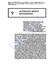
The placement of the language used in our experiments, within the Ethnologue language hierarchy.

. . . . . . . . . . . . . . . . . . . .

21

2.1

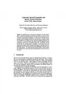
Workflow for training an HMM. . . . . . . . . . . . . . . . . . . . .

27

2.2

GMM upmixing workflow . . . . . . . . . . . . . . . . . . . . . . .

30

2.3

A 3-layer Multi-Layer Perceptron . . . . . . . . . . . . . . . . . . .

38

3.1

Workflow for one iteration of k-means clustering, done serially . . . .

47

3.2

Workflow for one iteration of k-means clustering, done in parallel. . .

47

3.3

Word error rate reduction against phoneme share factor . . . . . . . .

54

3.4

Word error rate reduction against triphone overlap . . . . . . . . . . .

55

3.5

Word error rate reduction against MLP frame error rate . . . . . . . .

56

3.6

Word error rate reduction against mutual information . . . . . . . . .

58

4.1

The effect of cross-corpus normalization on the MI of PLPs . . . . . .

65

4.2

The effect of cross-corpus normalization on the MI of MLP features .

66

4.3

WER and MLP FER against the proportion of language-independent MLP training data from the target language . . . . . . . . . . . . . .

4.4

WER and MLP FER against the share factor between target and source language for language-independent MLPs . . . . . . . . . . . . . . .

4.5

75

Frame error rates for German phoneme MLPs trained with varying amounts of data.

4.6

74

. . . . . . . . . . . . . . . . . . . . . . . . . . . .

78

Word error rates for recognisers using phoneme tandem where limited target language data is available. . . . . . . . . . . . . . . . . . . . .

80

5.1

Frame error rates for AF MLPs trained with varying amounts of data . 101

5.1

Frame error rates for AF MLPs trained with varying amounts of data . 102

5.2

Word error rates for recognisers using AF tandem where limited target language data is available. . . . . . . . . . . . . . . . . . . . . . . . 103 ix

6.1

Word error rates for phoneme tandem recognisers where limited target language data is available. . . . . . . . . . . . . . . . . . . . . . . . 109

6.2

Word error rates for various tandem recognisers where limited target language data is available. . . . . . . . . . . . . . . . . . . . . . . . 111

6.3

A summary of some cross-lingual tandem word error rates . . . . . . 112

x

List of Tables

1.1

Available multilingual speech corpora.

. . . . . . . . . . . . . . . .

1.2

The number of speakers in GlobalPhone in each corpus split, with gender, and the total size of the corpus in hours.

20

. . . . . . . . . . . . .

22

1.3

GlobalPhone lexicon sizes for each language. . . . . . . . . . . . . .

23

1.4

Phoneme distribution across languages. . . . . . . . . . . . . . . . .

24

2.1

Evaluating two-model training . . . . . . . . . . . . . . . . . . . . .

29

2.2

Baseline triphone GMM information . . . . . . . . . . . . . . . . . .

30

2.3

Word error rates for baseline MFCC-only systems . . . . . . . . . . .

32

2.4

Tuning lattice quality . . . . . . . . . . . . . . . . . . . . . . . . . .

32

2.5

Baseline lattice error rates . . . . . . . . . . . . . . . . . . . . . . .

33

2.6

Information about the MLPs used to classify phones in our tandem system and the corpora used to train them.

. . . . . . . . . . . . . .

39

2.7

Frame error rates for monolingual phoneme MLPs . . . . . . . . . .

40

2.8

Word error rates of monolingual baseline systems . . . . . . . . . . .

41

3.1

Word error rates for cross-lingual phoneme-tandem systems . . . . .

52

3.2

Share factors . . . . . . . . . . . . . . . . . . . . . . . . . . . . . .

54

3.3

Triphone overlap . . . . . . . . . . . . . . . . . . . . . . . . . . . .

55

3.4

A comparison of variables predicting cross-lingual performance of tandem features. . . . . . . . . . . . . . . . . . . . . . . . . . . . . . .

57

4.1

Evaluating cross-corpus normalization in terms of mutual information

63

4.2

Word error rates with and without cross-corpus normalization. . . . .

67

4.3

Information about the training of language-independent phoneme MLPs.

4.4

. . . . . . . . . . . . . . . . . . . . . . . . . . . . . . . . .

69

Word error rates for systems using language-independent phonemetandem features . . . . . . . . . . . . . . . . . . . . . . . . . . . . . xi

70

4.5

Feature vector sizes for a range of multilingual systems, plus monolingual systems for reference. . . . . . . . . . . . . . . . . . . . . . . .

4.6

Mutual information measure for a system using language-independent phoneme-tandem features . . . . . . . . . . . . . . . . . . . . . . . .

4.7

72

Share factors between various target languages and the source languages used for a language-independent MLP . . . . . . . . . . . . .

4.9

72

Proportion of target language data used to train a languageindependent MLP . . . . . . . . . . . . . . . . . . . . . . . . . . . .

4.8

71

73

Characteristics of German phoneme MLPs trained with varying amounts of data.

. . . . . . . . . . . . . . . . . . . . . . . . . . . .

77

4.10 Characteristics of language-independent phoneme MLPs trained with varying amounts of target language data.

. . . . . . . . . . . . . . .

77

4.11 Mutual information of normalized log-posteriors generated from phoneme MLPs trained with varying amounts of data.

. . . . . . . .

79

4.12 Word error rates for German recognisers using phoneme tandem trained with varying amounts of data. . . . . . . . . . . . . . . . . .

80

4.13 Comparing different PCA configurations for multiple-MLP phonemetandem systems in terms of word error rate. . . . . . . . . . . . . . .

84

4.14 Word error rates for systems using multiple-MLP phoneme-tandem features . . . . . . . . . . . . . . . . . . . . . . . . . . . . . . . . .

85

5.1

Articulatory features and their values. . . . . . . . . . . . . . . . . .

88

5.2

Articulatory feature MLP information . . . . . . . . . . . . . . . . .

89

5.3

Chance error rates for AF MLPs . . . . . . . . . . . . . . . . . . . .

89

5.4

Frame error rates for AF MLPs . . . . . . . . . . . . . . . . . . . . .

90

5.5

The resultant word error rates for two different PCA methods in AF tandem systems . . . . . . . . . . . . . . . . . . . . . . . . . . . . .

94

5.6

Word error rates for AF Tandem systems . . . . . . . . . . . . . . . .

94

5.7

Share factors of various labels used for language-independent MLPs.

95

5.8

Articulatory feature MLP information for Language-independent MLPs 96

5.9

Chance error rates for language-independent AF MLPs, reported for German, Portuguese and Spanish. . . . . . . . . . . . . . . . . . . .

96

5.10 Frame error rates for language-independent AF MLPs, reported for German, Portuguese and Spanish. . . . . . . . . . . . . . . . . . . . xii

97

5.11 Drops in frame error rate relative to their corresponding chance error rates, for language-independent and monolingual MLPs. . . . . . . .

97

5.12 Word error rates for a language-independent AF Tandem system . . .

98

5.13 Characteristics of German AF MLPs trained with varying amounts of data.

. . . . . . . . . . . . . . . . . . . . . . . . . . . . . . . . . .

99

5.14 Chance frame error rates for AF MLPs trained using just over four hours of German data.

. . . . . . . . . . . . . . . . . . . . . . . . .

99

5.15 Frame error rates for AF MLPs trained using just over four hours of German data. . . . . . . . . . . . . . . . . . . . . . . . . . . . . . .

99

5.16 Chance Frame error rates for AF MLPs trained using around 90 minutes of German data. . . . . . . . . . . . . . . . . . . . . . . . . . .

99

5.17 Frame error rates for AF MLPs trained using around 90 minutes of German data. . . . . . . . . . . . . . . . . . . . . . . . . . . . . . . 100 5.18 Word error rates for German recognisers using AF tandem trained with varying amounts of data. . . . . . . . . . . . . . . . . . . . . . . . . 100 A.1 Labels from each dictionary that are assumed to refer to the same IPA symbol. . . . . . . . . . . . . . . . . . . . . . . . . . . . . . . . . . 121 A.1 Distribution of articulatory features across languages — place of articulation. . . . . . . . . . . . . . . . . . . . . . . . . . . . . . . . . . 126 A.2 Distribution of articulatory features across languages — nasality.

. . 127

A.3 Distribution of articulatory features across languages — manner of articulation. . . . . . . . . . . . . . . . . . . . . . . . . . . . . . . . . 127 A.4 Distribution of articulatory features across languages — voicing.

. . 127

A.5 Distribution of articulatory features across languages — vowel rounding. . . . . . . . . . . . . . . . . . . . . . . . . . . . . . . . . . . . 128 A.6 Distribution of articulatory features across languages — vowel.

. . . 128

A.7 Distribution of articulatory features across languages — vowel stress.

129

A.8 Distribution of articulatory features across languages — vowel height.

129

A.9 Distribution of articulatory features across languages — vowel frontness.

. . . . . . . . . . . . . . . . . . . . . . . . . . . . . . . . . . 129

A.10 Frame error rates for language-independent phoneme MLPs . . . . . 130 A.11 Tuning lattice quality (detail) . . . . . . . . . . . . . . . . . . . . . . 131 A.12 The articulatory feature representations of the phonemes used. . . . . 135

xiii

Chapter 1 Introduction Automatic speech recognition (ASR) systems are typically composed of a number of components. Simply put, the stages are: Feature extraction In which the raw acoustic signal is represented as a sequence of vectors of real numbers. This representation is what makes the modeling of speech feasible. Acoustic model The acoustic model holds representations of sub-word units in terms of the feature space that we are operating in. The model needs to be trained with labelled data. Lexicon This is simply a look-up table which provides a correspondence between words and sequences of sub-word units. Language model This a model of word sequences, which allows us to select the most probable alternative out of those suggested by the acoustic model. Training acoustic models for speech recognition typically requires hundreds of hours of transcribed speech data (e.g. [Janin et al., 2007]). Whilst such data exist for English and a handful of other languages, there are thousands of languages for which there is only a little data [Gordon, 2005]. We are focusing on acoustic modelling and not other aspects of the recogniser — for instance, we assume a lexicon and language model exist for the language to be recognised. This work examines ways in which training data in one language can be used to improve the accuracy of a recogniser in another. That is done here by encapsulating information learnt from one corpus in the parameters of a model, which is then applied to the target language. 1

2

Chapter 1. Introduction

We do this by training a classifier, namely a neural network, on data in a source language and then applying it to recognise data in a target language. More than one source or target language can be used. Doing this directly requires either that the languages are labelled with a common set of sub-word units or that a mapping is learnt from the sub-word units in the source language(s) to the target language(s). Using the neural network output indirectly avoids the need for mapping between label sets. The terms directly and indirectly are more precisely defined in Section 1.3. The task that the neural network will perform is that of classifying the speech signal in to the sub-word units of the source language. Phonemes are the most commonly used sub-word unit, but perhaps phonemes are not the best classes to use for this task. When considering an alternative, it’s useful to bear in mind what properties we’re looking for: Realized in the same way in different languages This means that once a model has been trained in one language it can easily be applied to another. Since nominally identical phonemes (e.g. sharing the same IPA symbol) can in fact be realized differently in different languages [Imseng et al., 2011], phonemes may be a bad choice for cross-lingual recognition. Evenly distributed across languages For instance, we might train a classifier on a language which has few, or even zero, instances of a unit that occurs frequently in the target language — this would result in poor performance. Easily labelled Speech data usually have only word level transcriptions — the lexicon is then used to derive a phone-level transcription. Producing a dictionary for a new language can be a time-consuming and expensive task. In addition, for domains such as conversational telephone speech, the pronunciation observed is rarely the canonical pronunciation in the dictionary. Few in number and easily distinguishable These properties are desirable simply because they would make the classification problem easier. An alternative to phonemes that we will consider is articulatory features (AFs). Articulatory features are described in more detail in Chapter 5, but for our purposes they are a discrete multi-stream labelling of speech data that bears a close relationship to the physical articulators used for speech production. They have almost all of the desired properties listed above: they are a more language universal unit and should therefore have a more consistent representation across languages, they have similar coverage in

1.1. Usage scenarios

3

different languages ([Schultz and Kirchhoff, 2006, page 98] and Table 5.7). The classification problem can be posed so that multiple classifiers each have fewer classes to choose from. Previous work [Frankel and King, 2005] shows that AFs can be distinguished from each other using only acoustic observations. Another option is to use graphemes — this would mean simply using the letters that make up a word as its sub-word units. This solution has the advantage that the lexicon can be trivially generated, given a phonographic script. A disadvantage is that for some languages, e.g. English, the spelling can bear only little relation to the pronunciation. Due to time constraints, grapheme-based models are not used in this thesis. The rest of this chapter covers prior work in the area of cross-lingual and multilingual speech recognition, drawing in part from [Schultz and Kirchhoff, 2006, Chapter 4], which provides a good overview of work in multilingual acoustic modelling. Section 1.1 takes a look at various scenarios in which cross-lingual learning may take place, particularly looking at how the languages involved relate to each other, and identifies where the current work fits within the literature. Section 1.2 explores different choices of sub-word unit, namely contrasting the use of phonemes and articulatory representations. Section 1.3 then looks at different ways in which sub-word units could be represented in the model. Finally, Section 1.4 examines the different speech corpora that could be used, as well as the one that was eventually selected.

1.1

Usage scenarios

This section looks at different ways in which the language to be recognised and the other languages involved relate to each other. First of all we look at language independent systems, in which all languages involved are in the same position — the system can recognise more than one language and is trained with data from each of them. We then look at language adaptive systems, in which a model trained for one language is used in some way to aid the recognition of another target language — the resulting model can be applied to the target language but generally not to the source language.

1.1.1

Language-Independent

Language independent ASR systems are those which can recognise a number of different languages simultaneously. Some training data are usually available for each of

4


the languages and the models learnt are combined in some way. Methods for training both context-independent and context-dependent models are described below and are followed by the introduction of some work using a universal phoneset. Context-independent

In the case of context-independent models, e.g. monophones, there are three main ways in which acoustic models can be combined. The descriptions here assume phonemes to be an appropriate sub-word unit to use, but that need not be the case — the same methods could be applied to a different choice of unit. Heuristic Phonemes from different languages are treated as being in the same class as each other based on rules derived from articulatory knowledge [Weng et al., 1997], the IPA chart [Köhler, 1999] or auditory phonetic criteria [Dalgaard and Andersen, 1992]. A model for each class is trained using data from all languages and then used during decoding to model all phonemes within that class. Unless target language data is lacking [Andersen et al., 2003] or the ¨ speakers are bilingual/accented [Ubler et al., 1998] then a monolingual system using only target language data performed better than one using this heuristic mapping. Data-driven A similarity measure is used to cluster phonemes into classes. That measure could be something derived from, for example: • Confusion matrices obtained through recognition [Andersen et al., 2003] • The likelihood [Köhler, 1999] or posterior [Corredor-Ardoy et al., 1997] of a phone, given the model of another Recognition accuracy of a multilingual system trained in this way is worse than a monolingual system unless only limited amounts of data are available. Furthermore, the classes derived may not be linguistically meaningful and in some cases all sounds from one language end up in the same class. Hierarchical Phonemes are first separated into categories heuristically, and then some data-driven method is applied within those categories to cluster the models into the final set of classes used for recognition. In [Weng et al., 1997] phonemes in the same category share Gaussian components from single mixture model; in [Köhler, 1999] bottom-up clustering within IPA-based categories is used.


5

Hierarchical model combination, which essentially combines the two other methods, performs the best and using heuristic rules typically performs least well. Of course, none of the multilingual model combination methods described above performed better than a purely monolingual one. [Zgank et al., 2004] also compared a heuristic “expert-driven” phoneme mapping method to a data-driven (confusion matrix based) method for cross-lingual speech recognition and reached a similar conclusion.

Context-dependent

Whilst the previous section works with monophone (context-independent) models, we need some method that works with triphones (and other context-dependent units) since using triphones generally always provides an improvement over monophones.

Methods for training context-dependent models are described in

[Schultz and Kirchhoff, 2006, pp106–110]. ML-sep Separate models are trained for each phoneme and no sharing of data occurs between languages. The one exception to this (in [Schultz and Waibel, 2001]) is in the feature extraction stage, where LDA is used to maximize the separation between all phonemes and not just those for each separate recogniser. ML-mix Training data is shared across languages such that all phonemes sharing the same IPA symbol are treated as being the same phoneme. IPA phoneme labels are also referred to in questions when tying triphone models, but the language is not available as a potential question. ML-tag This differs from ML-mix in two ways • Data is labelled with its language, meaning that the triphone clustering procedure can ask questions about language • Gaussian components are shared between languages but mixture weights are trained separately As reported in [Schultz and Waibel, 1998], ML-tag outperforms ML-mix for the five languages that the methods were compared on. This implies that asking triphone tying questions about language is beneficial and it is not reasonable to assume that segments of speech from different languages with the same IPA symbol are the same.

6


Universal Phoneme Posteriors

In recent work presented in [Imseng et al., 2011], a universal phoneme classifier was used. MLP(s) were used to provide phoneme posteriors that were then modelled directly using an HMM. The phoneme posteriors used were derived in one of three ways: Monolingual A collection of monolingual MLPs, one per language. Universal : Language independent An MLP that classifies into a universal phoneset, consisting of the union of the phonesets of the languages involved. Language dependent A set three components, by which the posterior probability of a phoneme in the universal phoneset is estimated. The estimate is composed1 of: P(l|xt ) the frame-based language posterior P(u|mkl ) the probability of a universal phoneme given a language specific phoneme (this is assumed to be one if the phoneme symbols are identical and zero otherwise, i.e. a deterministic mapping) P(mkl,t |xt ) the posterior probability of a language specific phoneme The conclusions of the paper were that systems using universal phoneme posteriors (especially the language dependent system described above) were more accurate than the monolingual system when the language being spoken was unknown. Improved recognition of non-native speech was also reported.

1.1.2

Language Adaptive

The work in this thesis could perhaps be described as language adaptive — this refers to the scenario in which a model from a source language is applied to a target language. On the other hand, it does not take the form of the language adaptive method described in this section since the source language model does not directly appear in the target language model. Different terms exist for the cross-language scenarios that are possible: 1 The

expression used to estimate the posterior of universal phoneme u at time t is N

P(u|xt ) =

Kl

∑ P(l|xt ) ∑ P(u|mkl )P(mkl,t |xt ) l=1

k=1

where N is the number of languages and Kl the number of phonemes in language l.

(1.1)


7

Cross-language transfer This is the case where no target language training data is available.

Language adaptation technique Here, some target language data is available and is used to adapt a model trained from source language data.

Bootstrapping approach Bootstrapping is where plenty of target language data exists and so the source language data is used only to initialize the target language model. The target language data is then used to train the model.

Polyphone decision tree specialization (PDTS) [Schultz and Waibel, 1999] is an example of a language adaptive method and the starting point for a range of work in multilingual acoustic modelling. When combining context-dependent models from a number of different languages, the coverage of polyphones in the combined languages may differ widely from that in the language to be recognised. To address this, the decision tree learnt from the combined languages is specialized:

1. A multilingual polyphone decision tree is learnt using data from all input languages

2. Those phonemes not appearing the language to be decoded are removed from the tree

3. The tree is then regrown using some target language data until a specified number of leaves is attained

This final step means the distribution of polyphone contexts will diverge less from that which appears in the target language. The resulting decision tree is also specific to the target language being decoded. Whilst PDTS has been shown to work, this work focuses on the use of tandem features as method for applying the knowledge in one model to another.

8


The reasons for that decision include: • Cross-lingual transfer using tandem features allows for more separation between source and target languages — the units of the source language are of no concern to the target language model • The same tandem feature generation system can be used for a range of target languages • Little change is made to the target language model structure by the introduction of source language information (the differences are confined to the feature space) — this is arguably a simpler method

1.2

Sub-word Units

In order to directly share models across languages, the models need to be drawn from some common inventory of units. These will be the units that words are made up of and have been assumed up to this point to be phonemes. Other sub-word units could be considered and in the following sub-sections we look more closely at phonemes, articulatory features and briefly at graphemes.

1.2.1

Phonemes

Phonemes are by far the most commonly used sub-word unit used for ASR. The symbols themselves are generally derived from the IPA chart, with different subsets of IPA symbols being used for different languages. Using phonemes necessitates the use of a lexicon containing representations of words in terms of phoneme sequences. In reference to cross-lingual acoustic modelling, phonemes have advantages and disadvantages: Simple Many languages already have dictionaries that are expressed in terms of phonemes. Not realized uniformly across languages Although the same IPA symbol may be used in different languages they are not necessarily realized in the same way Less effective for conversational speech As discussed in [Ostendorf, 1999], it is difficult to transcribe spontaneous conversational speech in terms of phonemes be-

1.2. Sub-word Units

9

cause segments often apparently disappear or change. The canonical pronunciation that appears in the lexicon is rarely used outside read speech. Having multiple streams of articulatorily-motivated labels — rather than a single stream of labels, sometimes described as “beads on a string” — may allow us to capture various co-articulation effects that occur in spontaneous speech.

1.2.2


The use of articulatory knowledge in acoustic modelling is reviewed in [King et al., 2007]. The speaker’s articulatory state (i.e. the position and motion of lips, tongue and glottis) can be represented in the model in a wide variety of ways: Multi-valued categories This is where a number of feature streams, including for example, {place, manner, voicing, rounding, front-back}, are used. Each feature has a number of values it can take (for example, manner could be one of {lateral, nasal, fricative, approximant, vowel, silence}). Binary categories Here each feature is either present or absent rather than multivalued. The set of features is therefore larger and includes variables such as voiced/voiceless and nasal/non-nasal, as in the commonly used Chomsky and Halle features [Chomsky and Halle, 1968]. Tract variables In [Browman and Goldstein, 1992], speech is described in terms of gestures, i.e. constriction actions produced by the lips, tongue, velum and glottis. Speech gestures can be described in terms of eight tract variables2 , each of which is a physical position and its change over time. Formants Formants are peaks in amplitude on a spectral display of speech that vary as the speech signal changes. Whilst they do bear a relationship to speech production it is entirely mediated through the acoustic signal. Formants are simply a feature of spectrograms and not a physical concept that exists independently of them, unlike the other representations listed above. The position and movement of speech articulators can be physically measured in a number of ways: 2 These

variables are Lip Aperture, Lip Protrusion, Tongue Tip constriction (degree and location), Tongue Body constriction (degree and location), Velum and Glottis.

10


Electromagnetic Articulography Small magnetic coils are placed along the tongue, on the lips (and on the nose and upper incisors to provide stationary reference points). A magnetic field is used to induce currents in the coils, which are then measured. X-ray microbeam Here, gold pellets are used instead of using magnetic coils. These are observed with a narrow beam, high energy X-ray. Unlike the silent operation of EMA, the X-ray equipment used is noisy and so affects the audio recording quality as well as the naturalness of the speech. Electroglottograph Electrodes placed alongside the larynx measure changes in conductance, which imply changes in glottal contact area. Electropalatograph An artificial palate with a grid of electrical contacts is placed in the mouth to measure the position of contact between the tongue and the palate. Articulator positions can also be inferred from the acoustic signal, a process called articulatory inversion. A problem with using AF labels when training acoustic models is the issue of finding ground truth labels. These are usually derived by applying a simple mapping to pre-existing phone labels but doing so does not allow for the asynchrony that can occur between articulators in conversational speech. However, embedded training can be used to get a new realignment of the separate AF label streams. One attribute all of those articulatory representations share is their multi-stream nature. The multiple streams can either be represented explicitly in the model, e.g., with a multi-stream state space [Livescu et al., 2007], or implicitly, for example by concatenating the streams and passing them through a dimensionality reduction stage. AFs have been employed in a wide range of models: Additional acoustic features A number of experiments have shown that appending some representation of articulator positions to conventional acoustic features improves recognition accuracy. Those position can either be measured directly [Wrench and Richmond, 2000] (through, for example, electromagnetic articulography) or inferred (using, for example, an MLP [Fukuda et al., 2003]). The representation could be continuous, looking at how the exact positions of various points on the tongue change, or discrete, where a range of either binary of multi-valued phonetic features are used.

1.2. Sub-word Units

Hybrid models A

11

similar

but

slightly

different

scenario

[Kirchhoff, 1999,

Kirchhoff et al., 2002] is a hybrid HMM/ANN in which, rather than appending information on to the acoustic feature vector and then modelling that with a Gaussian Mixture Model (GMM), ANNs are used to provide likelihoods directly. Using a discrete, multi-stream articulatory representation, one MLP generates posterior distributions for each feature. Those distributions are then combined with a further MLP to give phoneme posteriors, which can be divided by prior probabilities to get likelihoods the HMM can use. Dynamic Bayesian Networks Dynamic Bayesian Networks (DBNs) are a class of probabilistic model, of which HMMs are one particular instance. DBNs allow the clear modelling of additional random variables, for example, articulator positions. In [Stephenson et al., 2000], a DBN is designed such that, at each time frame the observations are dependent on both the current sub-word state (as with HMMs) and on the current articulator position. The articulator position is observed during training but becomes hidden when decoding. Furthermore, the articulator position depends on the current sub-word state too, as well as the previous time frame’s articulator position. Using articulatory information in this model results in a 12 or 9% relative improvement in WER, depending whether it is treated as an observed or hidden variable respectively. Bayesian Network observation model In a hybrid HMM-Bayesian Network model [Markov et al., 2003] observations are modelled with a Bayesian network. Acoustic and discretized articulatory measurements are used, with the acoustic observations modelled using a GMM conditioned on both the sub-word state and the current articulator position. Training the model on both acoustic and articulatory data results in an improvement over just using acoustic data. Furthermore, decoding with that model using only acoustic data performs better than using a purely acoustic model. This work differs from that described in the previous paragraph in so far as there are no dependencies between AF variables in one frame and another. Linear Dynamic Models The previously described models employ a discrete representation of articulator position; an alternative would be to use a Linear Dynamic Model (LDM). An LDM has the same topology as an HMM, but with a continuous state variable. [Frankel, 2003] reports phone classification and recognition experiments using LDMs and measured articulatory observations.

12


In the context of prior work, this thesis can be positioned as the use of an abstract representation of the articulatory state as observations.

1.2.3

Graphemes

Whilst we do not use graphemes here, they do have some advantages that are relevant, as well as some obvious disadvantages Trivial dictionary creation One of the costs associated with recognising a new unseen language is that a dictionary needs to be created. If we use graphemes as our sub-word unit then that task can become much simpler — we consider the pronunciation of a word to be the sequence of letters in it. Only relevant for phonographic languages This clearly has limited applicability — it can not be directly applied to logographic languages such as Mandarin. Letter-to-sound mapping ignored The use of graphemes makes the largely unreasonable assumption that the spelling of a word directly implies the pronunciation. Whilst this may be partially true for some languages, e.g. Spanish, Japanese, it is not really the case for others e.g. English. Graphemes, articulatory features labels and phonemes like other sub-word units, can be either modelled directly or used indirectly, during training and decoding — those two options are explored in Section 1.3.

1.3

Modelling Methods

The sub-word units used could be represented in different ways — the contrast we look at here is between direct and indirect modelling. Direct models are those in which the units of the source language model appear explicitly in the target language model. The use of indirect models, on the other hand, means that the sub-word units from the source language do not necessarily appear in the target language model. Whilst with a direct model we would need sufficient target language training data for each of the source language units appearing in the model, that is not a concern in the indirect case — the set of units can be selected to be something more suitable for the target language.

1.3. Modelling Methods

1.3.1

13

Direct Modelling

Direct modelling means that the sub-word unit appears explicitly in the model structure and therefore requires a common inventory of unit types across all the languages involved. Examples include a conventional “HMMs-of-phones” system (as in Section 1.1) where source phonemes and target phonemes are drawn from a shared set of models, a hybrid system or a detector-based system (as described below). Hybrid Modelling

Phoneme-based hybrid models, in particular MLP-HMM hybrids, are first described in [Renals et al., 1992]. There, an MLP was used to provide class likelihoods for the DARPA Resource Management (RM) task [Price et al., 1988]. The MLP outputs were either used on their own or interpolated with GMM-derived likelihoods. For the 1k word vocabulary RM task, with a bigram language model, a baseline word error rate of 12.8% was attained — replacing the Gaussian mixtures for each state with an MLP brought that error rate down to 8.3%. Combining both models, by using a weighted sum of the class likelihood provided by each, gave a further reduction to 7.9% WER. Some of the benefits brought by using a hybrid ANN-HMM system include • access to a wider time context when determining phone likelihoods • the use of a discriminatively trained classifier A more complete description of hybrid ANN-HMM systems appears in [Bourlard and Morgan, 1993, Chapter 7]. Application to Articulatory Features

AF-based hybrid models had been used in [Kirchhoff et al., 2002]. In that work, separate MLPs were trained to give posterior probabilities for five different AFs — the outputs of those nets were then combined by being input to a further MLP. The posteriors from the merger MLP were used directly in the HMM. The AF hybrid system performed roughly as well as the phoneme-based system and significantly outperformed it under noisy conditions. Interestingly, different AFs deteriorated before others as the signal-to-noise ratio was reduced. The use of articulatory feature MLPs in a hybrid system was one of the aims of the 2006 Johns Hopkins Workshop and results of that work are presented in

14


[Livescu et al., 2007, Section 4.1]. The 10-word SVitchboard task was used to evaluate an AF hybrid system — SVitchboard [King, 2005] is a small vocabulary subset of a conversational telephone speech corpus. The AF MLPs used to produce phoneme posteriors were trained on around 2000 hours of data from the Fisher corpus [Frankel et al., 2007]. Experiments showed that a hybrid model performed worse than a monophone baseline, although that degradation reduced considerably when the model was used to realign the training data before retraining. Given the negative result it is suggested that hybrid models might perhaps be better suited to cross-lingual or cross-domain tasks.

Detector-based Speech Recognition

An

interesting

direction

that

is

relevant

to

this

work

is

covered

in

[Bromberg et al., 2007] — ASR based on an array of speech attribute detectors. A detector-based recogniser consists of three main stages [Siniscalchi et al., 2008]: 1. An array of detectors, each focusing on the task of detecting of a number of articulatory features, e.g. fricatives, stops or back vowels. These detectors can, and have been, implemented as MLPs. The input to this stage is an acoustic feature representation of the speech signal. Given a softmax output layer on the MLPs, the output is a posterior distribution for each articulatory feature. 2. An event merger stage, in which the attribute posteriors from the previous stage are combined to give phoneme posteriors. This is also implemented with an MLP, taking the posteriors from the first as input. 3. The final evidence verifier can also be thought of as an HMM decoder, common to many other ASR systems. Unlike some other articulatory feature based work, the work described in [Siniscalchi et al., 2008] treats AF detectors as a basic and central unit in the model.

1.3.2

Indirect Modelling

Indirect modelling, which is a focus of this thesis, means that the sub-word units used in training do not appear explicitly in the recognition model structure. The Tandem method is an indirect modelling approach, and is described this section.

1.3. Modelling Methods

15

Tandem Features

Tandem processing of features was introduced in [Hermansky et al., 2000] where it was applied to a noisy digit recognition task and then used for a noisy, mediumvocabulary spontaneous speech task [Ellis et al., 2001] (both in English). Tandem features are the concatenation of conventional acoustic features (e.g. MFCCs) to posterior probabilities provided by a discriminative classifier(s), after undergoing a dimensionality reducing transformation — the details of how they are extracted are described in Section 2.2. In [Ellis et al., 2001] two phone classifying MLPs were used to generate the posteriors used, each using a different acoustic feature set. Using tandem features resulted in substantial improvements when modelled with context-independent models and smaller but still significant gains after context was introduced and Maximum Likelihood Linear Regression (MLLR) applied. Adding tandem features to any ASR system typically brings a consistent improvement in accuracy, e.g. [Zhu et al., 2005]. Tandem systems have many of the advantages of the hybrid systems discussed in the previous section — access to a wider time context, use of a discriminatively trained classifier — but also allow us to benefit from advances in conventional GMM-based systems e.g., speaker adaptation methods or discriminative training. Another advantage of all indirect methods is that there is no requirement to devise a common sub-word unit inventory (e.g., a common phoneme set) for all the languages. The disadvantages include: this may somewhat restrict the potential for shared parameters between systems for different languages; the ASR system as a whole may be a little more complex. Application to Articulatory Features

The use of AF MLPs rather than phone MLPs to compute tandem features is described in [Çetin et al., 2007a]. There we see that, when supplied with the same training data, AF tandem features perform as well as phone tandem features on the SVitchboard 500word task. It was also shown that if better trained AF MLPs (i.e., trained on 2000 hours of data) are used then it results in a statistically significant improvement. Cross-lingual Use [C ¸ etin et al., 2007b]

Further work in [Çetin et al., 2007b] also uses AF MLPs in a

tandem system. As well as showing that a factored, multi-stream observation model

16


performs better than simply concatenating conventional and MLP features together, the paper features application to a cross-lingual system, with an English MLP being used to generate tandem features for a Mandarin broadcast news task. Focusing on the latter result, we see that whilst phone tandem features trained on English data bring down WER in the Mandarin system (from 21.5% to 21.2%), AF tandem features in fact degrade word error rate (21.9%). A number of possible explanations for the negative result with AF tandem features were given: • ground truth AF labels were unavailable for AF MLP training — AF labels were derived by applying simple rules to a phone-labelling produced by forced alignment with a pre-existing model • the acoustic features used for the AF MLPs may not be ideal for the task — additional acoustic-phonetic features such as fundamental frequency and voicing may be needed • the language mismatch is confounded by a domain mismatch — conversational telephone speech compared to broadcast news. [Toth et al., 2008]

Another example of tandem features being used cross-lingually

is [Toth et al., 2008], in which English phoneme MLPs and English AF MLPs3 are used to generate tandem features for a Hungarian telephony speech recognition task. As well as those two cross-lingual systems and monolingual tandem and non-tandem baselines, a system that used an adapted MLP was produced. The adapted MLP took the English phoneme MLP and retrained some model parameters with Hungarian data. Some results from that work include • Both English phoneme and AF MLPs provide an improvement over the nontandem baseline but do not perform any better than using tandem features from the Hungarian phoneme MLP. Domain and channel differences may have contributed to this result • Using the adapted MLP resulted in word error rates statistically significantly better than all other systems 3 Again,

the AF MLPs from [Frankel et al., 2007] that were trained on 2000 hours of Fisher corpus data were used.

1.3. Modelling Methods [Thomas et al., 2010]

17

In [Thomas et al., 2010] tandem features are used but the

cross-lingual element comes about through retraining of the MLP. The task addressed is the challenging Callhome corpus of conversational telephone speech. An MLP was trained to classify German and Spanish speech using a pooled phoneme set. It was then applied to English — output activations were observed as English speech was passed forward through the net and the mutual information between English phoneme labels and pooled German-Spanish phonemes was calculated. That information was used to learn a mapping between English and German-Spanish phonemes and the MLP underwent further training with a limited amount of target language data, now relabelled with German-Spanish phonemes. Recognition accuracy is shown to improve with the use of non-target speech data. The main differences between that work and ours is in the use of MLP training as the tool for cross-lingual transfer as well as their extensive use of novel acoustic features. [Rasipuram and Magimai-Doss, 2011]

[Rasipuram and Magimai-Doss, 2011] fea-

tures the use of articulatory feature posteriors in a Kullback-Leibler divergence based HMM (KL-HMM). A typical KL-HMM takes phoneme posteriors at each frame and computes the KL-divergence between them and a reference multinomial distribution defined for each state. The state sequence that minimizes the total KL-divergence is found by Viterbi decoding. This paper showed that by using a multi-stage series of AF MLPs to estimate AF posteriors it is possible to perform phoneme recognition as accurately as with phoneme MLPs on the TIMIT corpus. Furthermore, AF posteriors can easily be combined with phoneme posteriors in a KL-HMM system to give an improvement in accuracy relative to a phoneme posterior only system. Template Matching

Features based on class posteriors have been used within the template matching paradigm too [Aradilla et al., 2008]. Without giving a detailed explanation, template matching is a method for performing speech recognition that differs a great deal from conventional HMM-based recognition. Words are treated as sequences of feature vectors and typically dynamic time warping is used to compare candidate words against templates learnt from data. In [Aradilla et al., 2008], a feature space consisting of phoneme posteriors is used and compared with a more conventional PLP feature space. This allows the principled

18


use of Kullback-Leibler divergence ([Mackay, 2003] and related measures) to calculate the distances to templates — since the feature space consists of posterior distributions all elements sum to one and are non-negative and KL-divergence takes account of that. Whilst a highly interesting and novel approach, it is difficult to draw further comparison between the use of posterior features in template matching and ours.

Subspace GMMs

An exciting new model for speech recognition is that of Subspace Gaussian mixture models (SGMMs). In a subspace GMM, the distribution of acoustic features x for state j is modelled with a Gaussian mixture: P(x| j) = ∑Ii=1 w j N (x; µ ji Σi ). I is typically a few hundred, covariances are shared across states. The interesting difference with subspace GMMs is that the mean vectors are estimated separately and defined as µ ji = Mi v j . Mi describes the subspace in which mean vectors can live and v j appears to represent the range of speech sounds [Burget et al., 2010, Figure 1]. In [Burget et al., 2010], SGMMs are applied to the task of multilingual speech recognition. The English, Spanish and German parts of the challenging Callhome corpus are used. The shared parameters Mi are the focus here — in the mulitlinugal system those parameters are trained with data from all three languages; the state-specific v j are trained with language-specific data. That approach results in 1.5%, 0.5% and 1.0% absolute improvements in word error rate for English, Spanish and German recognisers respectively when compared to a monolinugal SGMM recogniser. Also, when only limited amounts of target language data are available, using data from other languages to train the shared parameters results in a substantial drop in error rate. An English recogniser with only one hour of training data sees a drop in word error rate of 8% absolute if the Spanish and German corpora are also used for the estimation of shared parameters. Some similarity with the work described in this thesis can be seen since information is being transferred between languages through the trained parameters of a model — in this case it is through the shared Mi matrices and in cross-lingual tandem it is through MLP parameters.

1.4

Data

All of the methods discussed so far require at least a few hours of transcribed speech data if we are to learn and evaluate probabilistic models of speech. The speech corpora

1.4. Data

19

would need to be in a number of different languages and with word-level transcriptions. Recordings of native speakers are strongly preferred. Individual speech corpora recorded for different tasks and under different conditions already exist and could be used for this task. However, doing so would mean that, in addition to cross-lingual differences, there would be further differences introduced by disparities in task (effecting e.g. vocabulary and utterance length) and recording conditions (e.g. telephone vs. studio recordings, noisy vs. quiet conditions). To avoid that unnecessary additional factor of cross-corpus normalization4 , we restrict our corpus choice to one of several multilingual corpora available — some of them are described in Table 1.1. The GlobalPhone corpus was chosen because it contained enough data in each language for a baseline recogniser to be built and because it contained a wide range of languages. Ten of the available languages were selected such that a wide range of phonetic phenomena are seen and some groups of similar languages exist, but so far experiments have only been performed with six of them, due to the unavailability of language models for the other four. Our choice of languages covers a range of language families — their relation to each other is described in Figure 1.1. The phonetic characteristics of each of the language families included, in particular those aspects that differ between families, are briefly given below. A wide and distinct set of phonetic phenomena exhibited in source and target languages is one of the challenges faced in cross-lingual speech recognition and so choosing a set of languages with a diverse range of properties should force us to address that. Chinese In Mandarin Chinese, syllables consist of a vowel nucleus, which can be a monophthong, diphthong or triphthong, and optional an onset and coda. The tone of the vowel is phonemic. Consonant clusters are rare in the syllable onset. In Mandarin, only /n/ and /N/ are valid codas. [Chao, 1968] Germanic Swedish features a unique voiceless palatal-velar fricative realization of /Ê/ [Ladefoged and Maddieson, 1996, pages 171–2, 330; 173–6].

It

also possibly has more than on type of lip rounding gesture in vowels [Ladefoged and Maddieson, 1996, page 295]. Both German and Swedish have phonemic vowel length. German and Russian have broadly similar movement patterns for labiodental fricatives [Ladefoged and Maddieson, 1996, page 140]. 4 Despite

using a multilingual corpus recorded under consistent conditions we still put some work into normalization — see Section 4.1.

20


Corpus

number Notes of languages

GlobalPhone[Schultz, 2002]

up 15

to

Includes English, Arabic, Chinese and a number of European languages. 300+ hours total data.

OGI

Multi-language

Telephone

11

Speech

2052 speakers and about 40 hours total data.

Corpus[Muthusamy et al., 1992] EPPS[ELRA, 2006]

5+

Recordings of European Parliament Sessions.

92 hours of transcribed

speech. SPEECON[Siemund et al., 2000]

10

Some European languages plus Mandarin and Korean.

Estimated 300

hours total data. EUROM1[Chan et al., 1995]

11

European languages including English. 60 speakers per language. Estimated 18 hours per language (about 200 hours total).

AURORA3[Pearce et al., 2000]

5

Isolated and connected digits recorded in a car; European languages.

Table 1.1: Available multilingual speech corpora.

1.4. Data

21

• Indo-European – Germanic ∗ North → East Scandinavian → Danish-Swedish · Swedish ∗ West → High German → German → Middle German → East Middle German · German – Balto-Slavic ∗ Slavic → East-Slavic · Russian – Italic ∗ Romance → Italo-Western → Western → Gallo-Iberian → IberoRomance → West Iberian · Portuguese-Galician → Portuguese · Castilian → Spanish • Sino-Tibetan – Chinese Figure 1.1: The placement of the language used in our experiments, within the Ethnologue language hierarchy.

22


Number of speakers Language

Training

Development

Evaluation

Total(hours)

M

F

Σ

M

F

Σ

M

F

Σ

Chinese

53

58

111

6

5

11

5

5

10

31

German

62

3

65

4

2

6

4

2

6

18

Portuguese

45

41

86

4

4

8

4

3

7

26

Russian

51

44

95

5

5

10

5

5

10

22

Spanish

34

45

79

5

5

10

4

4

8

22

Swedish

40

39

79

5

4

9

5

5

10

22

Table 1.2: The number of speakers in GlobalPhone in each corpus split, with gender, and the total size of the corpus in hours.

Romance Spanish

has

an

alveolar

trill

/r/

that

Russian[Ladefoged and Maddieson, 1996, page 218].

also

appears

in

Spanish is unusual

amongst the world’s languages in having dental fricatives[Harris, 1969]. An uncommon aspect of Portuguese is that, whilst laterals in most languages have some place of articulation, it has completely unoccluded laterals [Ladefoged and Maddieson, 1996, page 193]. Russian Russian has five vowels and a set of consonants that come in plain and palatized pairs, known as hard and soft consonants [Halle, 1959]. Syllable-initial consonant sequences are common [Ladefoged and Maddieson, 1996, page 128] GlobalPhone consists of recordings of a range of speakers reading from a newspaper in their native language. Recording were done under a range of ‘quiet’ conditions using a Sony DAT-recorder TDC-8 and a close-talking Sennheiser microphone HD440-6 — since the recording locations varied, acoustic conditions are likely to vary both between and within each language corpora. The amount of data available in each language, as well as the standard partitioning into training, cross-validation (dev˙) and test, plus the gender split of the speakers is described in Table 1.2. The sizes of the available GlobalPhone lexica in each language are given in Table 1.3. The phoneme inventory for each language is described in Table 1.4. At the conclusion of this chapter we have introduced the task we wish to address and the corpus we will be working with. We will be performing cross-lingual automatic speech recognition using an indirect model to transfer knowledge between languages.

1.4. Data

23

Language

Pronunciations

Words

Chinese

73388

73387

German

48979

46037

Portuguese

54163

51987

Russian

28818

27062

Spanish

41286

28803

Swedish

25402

25257

Table 1.3: GlobalPhone lexicon sizes for each language.

Our sub-word units for the model will be phonemes but articulatory feature based units will also be used when a model is transfered from one language to another. We will use six languages from the GlobalPhone corpus, each language in the corpus has around 20 hours of clean newspaper text read by native speakers. The following chapter goes on to describe some baseline experimental results, arrived at by using the methods and data introduced in this chapter.

24


Shared

Number of

by this

phonemes

Polyphonemes

many languages Consonants

Vowels

All

10

f, k, l, m, n, p, s, t

i, u

5

7

b, d, g, r

a, e, o

4

5

j, S, v, x, z

3

4

N, ð, ts

y

2

29

ç, dj , L, ù, tj , ü,w

E, ai, a:, ä, 5, au, ei, e:, ë, 9, eu, i:, ï, O, ø, ø:, o:, o¨, y:, u:, u¨

Language Number of

Monophonemes

monophonemes (total phonemes) CH

24(45)

kh , C, th , tsh , tù, tùh ,

A,AU, AI, ia, iAU, iE, iO,

tC,tCh

iou, ou, 7, ua, uaI, uei, yœ, uO

GE

1(44)

-

5

PO

15(48)

K

ã, "ã, 5, ˜e, "˜e, ˜i, "˜i, I, o˜, "õ, u˜, "˜u, U

RU

16(49)

bj , lj , mj , pj , P, rj , sj , C:, W C:j , zj , üj , Sj , ts, tsj , vj

SP

8(43)

D, G, ð, R, T, tS, B

oi

SW

14(52)

ã, ks, í, ï, ú

A:, E:, æ, æ:, O, œ, œ:, 8, 0:

Σ

78

Table 1.4: Phoneme distribution across languages. This table is in fact a version of [Schultz and Kirchhoff, 2006, Table 4.3] limited to the six languages used here. Polyphonemes are phonemes appearing in more than one languages, monophonemes appear in only one.

Chapter 2 Baseline systems In the previous chapter we defined the problem we intend to address and the datasets that will be involved. As with any evaluation, we need a baseline system with which to compare our new methods and in this chapter we state some baseline results and describe how those models were created. This chapter describes two baseline systems — Section 2.1 describes a GMM-HMM system built using only conventional MFCCs (Mel Frequency Cepstral Coefficients) as acoustic input and Section 2.2 looks at a simple, monolingual tandem system (in which MFCCs are supplemented with MLPbased features).

2.1

Conventional acoustic features

A conventional GMM-HMM system was built to provide: • a baseline for comparison with tandem systems • phone-level alignments used for training the classifiers used in future steps The remainder of this section describes how that model was trained and how it performed on test data.

2.1.1

Model training

This, and all other HMM systems described here, were created using HTK [Young et al., 2006]. Standard MFCC acoustic features1 were extracted and speakerlevel cepstral mean and variance normalization was applied. 1 MFCC

E D A Z in HTK notation

25

26

Chapter 2. Baseline systems

The workflow used to train the baseline model is described in Figure 2.1, with notes below — it is based on the tutorial recipe in the HTKBook [Young et al., 2006, Chapter 3]. 1. Initialization. A flat start initialization is used to set the starting parameters of our model. Each phone is modelled with an HMM that has three emitting states. The emission model in each of those states is a diagonal covariance Gaussian. The variance floor is also set here — during training, no covariance element is allowed to fall below its floor value. An additional special model is used to deal with out-of-vocabulary (OOV) words — words in the training corpus that do not appear in the lexicon are given this phone as their pronunciation and an unknown word , with the special label as its pronunciation, is used during decoding to catch OOVs in the test data. 2. Expectation Maximization Given the existing word-level transcription of the training corpus, a lexicon with exactly one pronunciation for each word is used to generate a phone-level transcription. Each pronunciation in the lexicon ends with the silent phone sil meaning that we assume, for now, that all words have some silence after them. EM training continues until the increase in the average log-likelihood per frame of the training data falls below some convergence limit (5% relative increase). 3. Inter-word pauses The centre state of the silent phone is cloned to create a one state short pause (sp) model. This sp symbol appears at the end of all pronunciations in the lexicon that is used from here on. The topology of the sp HMM is such that the emitting state can be skipped, making the pause between words optional. 4. Align The new HMM with an sp model undergoes EM-training, iterating until the relative increase in training data likelihood falls below 5%. A forced alignment of the training data is performed using the trained model and the new lexicon described in the previous step. This gives us a phone-level alignment. 5. Upmix The HTK PS command is used to split the Gaussian mixture components and turn the existing single Gaussian system into a GMM. The number of Gaussian components per state is proportional to the number frames of speech for that state, raised to some power2 . Splitting is done in three steps, with EM-training 2 The

value of 0.2 used, taken from the example in HTKBook.

2.1. Conventional acoustic features

Initialize model (1)

EM-training of monophones (2)

27

Clone (8)

EM-training of triphones

EM-training of triphones (10)

Inter-word

State-

State-tying

pause (3)

tying (9)

(11)

EM-training

EM-training

of tied

of tied

models

models

Upmix

Upmix

Align (4)

Upmix (5)

Align (6)

EM (7)

Figure 2.1: Workflow for training an HMM.

28


after each of those split stages (see Figure 2.2). The first round of EM-training continues until the relative likelihood increase falls below 0.5%, the other two rounds consist of just one iteration. An average of 128 components per state is used for the monophone model in all languages. The number of components in later triphone GMMs varies between languages, depending on dev. set WER, and is described in Table 2.2. To avoid problems brought about by trying to create too many components at once, the following gentle upmix schedule was employed — 1 2 4 6 8 10 12 15 18 21 24 28 32 48 64 96 112 128 — and component weights are floored3 to 5×MINMIX. 6. Align The monophone GMM is used to perform a forced alignment of the data. 7. EM Using the alignment generated from the monophone GMM, re-estimate parameters for the single Gaussian monophone model 8. Clone The lexicon is used to enumerate all possible cross-word triphones — these triphones are initialized to be clones of their centre phone’s single Gaussian monophone model. 9. Tie Decision tree tying is used to tie those trained models — standard questions about the neighbouring phones are used. Tree growth is managed by two parameters — the minimum increase in log-likelihood required for a question to be asked (i.e. for a new tree node) and the minimum size (in terms of state occupancy) of a leaf node (nodes falling below the minimum will be pruned). The min. increase was set to 900 and the outlier threshold was 100. Triphones that are unseen in the lexicon or training data transcriptions are synthesized using this tree. 10. Two-model re-estimation is used in this recipe – this means that the model used to align the initial, cloned triphone is a fully trained tied-triphone system. This improves on simply using the monophone GMM to align the model, which would have a less precise correspondence between frames of speech and phone labels [Young et al., 2006, Section 8.7]. The resultant model is shown to be more accurate in Table 2.1. 11. Tie The second state-tying operates in the same way as the first but, given the improved alignment used to train the initial cloned triphones, the occupancy 3 using

the -w option on HERest


29

Word error rate (%) Language

conventional

two-model training

Chinese

23.1

23.3

German

26.4

26.1

Portuguese

27.3

23.5

Russian

34.2

34.7

Spanish

19.0

18.3

Swedish

50.8

50.3

Table 2.1: Using two-model training results in an improvement in accuracy for most languages (LM scale & insertion penalty have not been tuned for the conventional system, so the improvement may diminish for some languages). Eval. set word error rates are shown.

statistics will be different and a different tree will result. The actual number of physical triphones in each system is given in Table 2.2. For reasons of consistency the same workflow is used throughout — regardless of the languages involved or feature set used, the same process is employed. Parameters that vary between systems, aside from feature-set related parameters, are: • The number of Gaussian components per state in the aligning model at step 8 • The number of Gaussian components per state in the final model • Decoding parameters: – Insertion penalty – Language model scale As well as the acoustic model, we need a language model (LM) for use during decoding. Standard n-gram language models, which were available from the same source as the GlobalPhone corpus, are used. The LM provides the probability of a word given the previous n − 1 words. That probability is multiplied by a grammar scale parameter when it is combined with the acoustic model score — that parameter is something that is tuned to minimize the dev. set word error rate. Both a bigram (supplying P(wi |wi−1 )) and trigram (supplying P(wi |wi−1 , wi−2 )) models are available.

30


Language

number of components

number of triphones

Chinese

24

1985

German

15

3653

Portuguese

18

2436

Russian

12

1836

Spanish

24

1546

Swedish

10

3221

Table 2.2: Some details about the baseline triphone GMMs, namely — the mean number of Gaussian components per state and the number of physical triphones.

from previous iteration

Split

EM

Split

EM

Split

EM

Upmix to next iteration Figure 2.2: Workflow for upmixing Gaussian mixture models. The diagram describes the process for going from, say, 15 to 18 components per state. Each Split block represents one of the three partial PS commands. The same method was used for throughout.


2.1.2

31

Results

Decoding was performed using these models to obtain the results in Table 2.3. A two-pass method was employed: 1. Lattices were generated using HDecode. Search parameters were selected to optimize dev. set lattice error rate — the Swedish corpus was used here and the same tuned parameters used throughout. Table 2.4 describes that tuning — in summary it shows that • a wider beam adversely affects run-time with little improvement in accuracy. That is, if the correct hypothesis is available at all, then it has high likelihood and widening the beam is unnecessary. • increasing the number of tokens per state improves accuracy but also requires more run-time 2. The 1st best path through the lattice is found. Whilst a bigram language model was used in the first step, those LM scores are discarded and probabilities from a trigram model are used instead. A rough manual search was used to find the grammar scale and word insertion penalty that minimized the word error rate of the 1st best hypotheses in the dev. set. The search method only goes as far as to guarantee that increasing or decreasing the LM scale and/or insertion penalty by 4 will result in an increased error rate, that is, we are at a minimum. This was the first method implemented and whilst better ones could have been used. The fact that • earlier searches exploring wider values for scale & penalty only found higher word error rates and • similar values are found across different languages implies that the optima found are not simply local optima. The same scale and penalty was used when searching for the 1st best path through the eval. set lattices. Scale and penalty were tuned separately for each language but the same beam was used to generate lattices across all languages. One important observation to be made here is that Swedish has a very high word error rate, especially in comparison to recognisers performing the same task in the other GlobalPhone languages. The same recipe that created effective recognisers in other

32


Word error rate (%)

Language

dev

eval

Chinese

17.2

23.3

German

26.9

26.1

Portuguese

26.1

23.5

Russian

38.8

34.7

Spanish

27.3

18.3

Swedish

49.4

50.3

Table 2.3: Word error rates for baseline MFCC-only systems. In Chinese, pinyin error rates are quoted, and not word error rates.

tokens/state(-n)

beam(-t)

word-end beam(-v)

Lattice

Real-

error

time

rate(%)

factor

10

500

50

45.38

8.5

10

500

100

34.23

10.7

10

500

200

30.58

12.9

10

750

50

44.20

24.4

10

750

100

33.52

31.9

10

750

200

30.00

28.6

15

500

200

26.16

17.8

20

500

200

23.44

20.2

25

500

200

21.57

22.3

32

500

200

19.91

28.0

50

500

200

16.67

46.1

64

500

200

16.52

64.1

Table 2.4: Lattice error rates for the Swedish dev. set at various lattice sizes and beam settings, with mean real-time factors shown. HDecode flags are shown in column headings, for reference. A fuller version of this search appears in Table A.11.

2.2. Baseline Monolingual Tandem

Language

33

Lattice error rate(%) dev

eval

Chinese

51.7

43.7

German

13.7

13.8

Portuguese

15.3

16.7

Russian

20.9

14.3

Spanish

12.5

9.8

Swedish

19.9

21.9

Table 2.5: Lattice error rates (the word error rate of the path through the lattice with the lowest word error rate) for baseline MFCC-only systems. In Chinese, the error rates are word error rates, not pinyin error rates. In Russian, utterance RU065 34 is excluded for lattice error rate calculation due to excessive length.

languages was used for Swedish so it is difficult to find the cause of the problem. Further attempts to debug the problem were unsuccessful and so any conclusions drawn in this thesis will be made without reference to Swedish results. The Russian recogniser also has quite a high error rate, this has been ascribed to the language’s rich morphology [Stüker and Schultz, 2004, Section 4.6] and possible deficiencies in the lexicon4 . Furthermore, the results achieved here are comparable to those in [Stüker and Schultz, 2004]. This becomes relevant later when we choose to work with only a subset of these six languages.

2.2

Baseline Monolingual Tandem

Tandem modelling [Ellis et al., 2001] can be seen as a (rather complex) preprocessing/feature extraction step to produce the observations for a conventional generative Gaussian mixture model. Now that we have a reasonably effective MFCC based recogniser we can use it to produce phone-level labels for the generation of tandem features. This mono-lingual baseline serves as a point of comparison for cross-lingual systems. The steps required 4 Following

discussions with a Russian speaker, Korin Richmond.

34


to generate a model that uses tandem features are described below:

1. Train the MFCC baseline system, as described in Figure 2.1 Training MFCC Tune Train Data Dev.

GMMHMM

MFCC

Data

2. Generate a frame-level phone labelling for the corpus by forced-alignment of the MFCC baseline model made in the previous step. This step also requires a word-level transcription and a lexicon that maps from words to phoneme. GMMHMM Data

Forced

MFCC

Labels

phoneme Labels

Alignment word

3. Train an MLP using frame-level targets obtained from the previous step. PLPs5 are extracted from the acoustic data instead of MFCCs. phoneme Labels Training PLP Data Dev. Data

5 PLP

E D A Z in HTK notation

Train PLP

Convergence Test

MLP


35

4. Generate tandem features: (a) Apply that trained classifier to the corpus and obtaining estimated phone posteriors at each frame. (b) Take logs of those posteriors. This is equivalent to omitting the softmax function that is usually applied in the output layer of the net. Taking logs results in features that appear more Gaussian. (c) Transform them using, for example, PCA. PCA is used to decorrelate and reduce the dimensionality of the features that are going to be concatenated — using HLDA (Hetroscedastic Linear Discriminant Analysis, [Kunar, 1997]), or any other similar scheme is also an option here. The PCA transform is estimated using the training set. The number of dimensions is reduced such that 95% of the variance is still accounted for.6 The features generated at this point will be referred to as MLP features, to distinguish them from log-posteriors generated in the previous step and tandem features generated in the following step. (d) The massaged MLP output vector is now concatenated to the MFCCs. These acoustic features can be the same as those input to the MLPs but a further gain in performance can be attained if complementary acoustic features are used, e.g. the MLPs are trained with PLPs and MFCCs are used in this step. MLP MLP

forward

PLP

Data

pass POSTERIORS PCA

MFCC Concatenate

TANDEM

Data

5. The new features can be modelled with a GMM-HMM again using the training schedule described in Figure 2.1 Training TANDEM Data Dev.

Train

Tune

GMMHMM

TANDEM

Data Once tandem features have been generated, decoding is performed in the same way 6 This

conveniently means that we can fairly compare systems built using different numbers of sub¨ ur Çetin. word units. A script to implement this heuristic was provided by Ozg¨

36


as with an MFCC-based model. Adding tandem features to a system has been shown to consistently improve recognition performance. This happens for a number of reasons: • Since acoustic observations from a number of frames either side of the one being classified are input to the MLP, it can bring in information from a wider time context. • The classifier has been trained discriminatively, in other words to minimize error, rather than with any other objective e.g. maximizing likelihood. A number of effective extensions to the basic tandem system have been made, some of them include: • TRAPs (TempoRAl PatternS, [Hermansky and Sharma, 1998]) and subsequently HATS (Hidden Activation TRAPs, [Chen et al., 2003]) operate by using a long window of the log spectrum over a single frequency band. In a system using TRAPs, features from a window as long as 1 second would be fed to an MLP, with one MLP existing per frequency band. The outputs of those classifiers would then be combined in a further MLP to give a phone posterior. HATS works in the same was as TRAPS except that the output layers of the frequency band MLPs are removed and the activations of the hidden layers are used in their place. • Using state posteriors rather than phone posteriors as the targets for the MLP has been shown to result in better accuracy [Grézl and Fousek, 2008]. Apart from requiring a state-level alignment of the training corpus for MLP training, this is an easy modification. • Bottle-neck MLPs [Grézl and Fousek, 2008] are four or five layer MLPs in which the middle layer has far fewer units than the other hidden layers (which are large as usual). The smaller layer is the bottle-neck layer. The MLP is trained as usual to perform phone classification, but when it comes to using it for tandem feature generation the activations of the bottle-neck layer are used instead of the output layer. Modifications to tandem feature generation are not the focus of this thesis and so the standard workflow is used.


2.2.1

37

Multi-layer Perceptrons

Phone posteriors in our tandem systems are provided by multi-layer perceptrons (MLPs).

Training and classification were both performed with QuickNet

[Johnson et al., 2011]. The input to the MLP consists of the PLP coefficients at the frame to be classified and at the adjacent four frames in either direction — a nine frame context window. At the beginning of each utterance the left-hand context consists of some padding frames, — the first frame repeated four times. A similar fix is applied at the end of each utterance. Training MLPs

We use three-layer feed forward MLPs (a simple example appears in Figure 2.3) and train them in the conventional way, using back-propagation to minimize errors on the training set. Training consists of two steps, jointly referred to as an epoch, that are iterated through until the frame error rate on a cross validation set (identical to the dev. set mentioned elsewhere) converges. Propagation New training patterns are presented to the network — in a batch update setup as used here, multiple patterns are presented before weights are updated (the exact number of patterns is discussed below on page 39). Forward The input is passed forwards through the network and the current weights are used to give output activations at each layer Backward At the output layer, the activations are compared with ground truth training targets to give deltas Update For each weight • Compute the gradient at that point using previously computed deltas • Using the gradient to determine which direction would reduce error, update the weight in that direction by moving an amount proportional to the learning rate set The initial learning rate used when training MLPs was 0.005. The “newbob” learning rate schedule was used, meaning that after starting with the initial learning rate we repeat epochs until the dev. set frame accuracy increases by less than 0.5% over the

38


Input

Hidden

Output

layer

layer

layer

Input #1 Input #2 Input #3 Input #4

Figure 2.3: A simple 3-layer MLP, as used to generate the class posterior probabilities used for tandem processing. The number of nodes in the output layer is equal to the number of classes, that is, the number of phonemes. The number of input nodes is the product of the number of features per frame and the number of frames in the input window. The size of the hidden layer can be adjusted to give various levels of model complexity.


Language

39

units in layer

free parameters

Training data

Training

hidden

as % of data

(×106

time (×103

frames

frames/×104 sec)

sec)

(×103 )

output

Chinese

12.1

44

50

9.30

89.3

German

4.85

44

35

5.25

17.3

Portuguese

8.35

48

40

8.06

45.6

Russian

8.07

45

45

6.71

50.0

Spanish

8.00

43

50

6.05

36.4

Swedish

7.11

52

45

6.13

29.2

Table 2.6: Information about the MLPs used to classify phones in our tandem system and the corpora used to train them.

previous epoch. After that, the learning rate is halved before each epoch to home-in with increasing precision on the local optimum7 . The number of units in the hidden layer is set such that the number of free parameters in the net is equal to some percentage of the total number of data frames8 . The number of free parameters in a net with a I × H × O structure is I + H + O + H(I + O) where I is the product of the number of features per frame (39 PLP coefficients) and the size of the context window (9 frames) and O is the number of phonemes in the language being classified. The actual percentage used was around 35–50% but was tuned to each language so as to maximize dev. set accuracy. A softmax output function is used so that output nodes sum to one and can be treated as the posterior probability of that class being the label for the current frame. MLPs throughout are gender-independent. The presentation order of the training data is randomized, so as to avoid local minima. A batch update of the parameters is applied during training after each ’chunk’ of data is processed. The chunk size is determined dynamically by a simple heuristic which refers to the memory available on the executing machine. Chunk size is selected to be as large as can be held in memory but also such that the final chunk is not small (a small final chunk would bias the estimated parameters towards the data appearing in that less representative chunk).

7 http://www.icsi.berkeley.edu/speech/faq/nn-train.html 8 This

heuristic was provided by Joe Frankel

40


Language

Frame error rate(%) MLP dev

Phone error rate (%) [Schultz and Kirchhoff, 2006, Fig. 4.5],

eval [Schultz and Waibel, 2001, Fig. 4]

Chinese

31.2(32.2)

34.6(35.6)

45.2

German

26.5(30.6)

25.2(29.2)

44.5

Portuguese

47.7(49.4)

41.1(42.4)

46.8

Russian

38.4(39.5)

37.5(38.6)

50.79

Spanish

31.8(32.6)

29.0(29.8)

43.5

Swedish

39.6(41.3)

37.4(39.2)

-

Table 2.7: Frame error rates for all used languages are reported here — ignoring the silence class gives the figures in parentheses.

Classifying with MLPs

Classifying with an MLP is relatively straightforward. The weights and biases in each layer of the MLP have been set by the training stage and remain unaltered. In the MLPs we use here the output layer has a softmax activation function and so the output unit with the highest activation is the one with the greatest posterior probability. The label corresponding to that unit can be taken to be the label for that frame. Table 2.7 shows the performance of the language-specific MLPs described in Table 2.6 (since silence is very easy to classify and, at the same time, not very useful, frame error rates in which all frames labelled as silent in the reference labelling are ignored are also given). It would be useful to have some benchmark against which to compare those error rates. Unfortunately, we were unable to find any phone classification results for the GlobalPhone corpus — we do however have phone recognition figures from [Schultz and Kirchhoff, 2006, Fig. 4.5, p. 86] and [Schultz and Waibel, 2001, Fig. 4]. A rough comparison with those results implies that our MLPs are not under-performing. Since the MLP is not being used as a classifier, but to generate a vector of features, the identity of the class with maximum posterior probability is not the only quantity of interest. Maximizing the difference between the highest posterior and all others can be expected to result in better tandem features. It should also produce distinct posterior distributions when applied to different speech segments in a language it may not have


41

been trained to classify.

2.2.2

Results

Looking at Table 2.8 we can see that tandem features result in a consistent improvement in recognition accuracy. The matched pairs sentence-segment word error statistical significance test [Gillick and Cox, 1989], implies that at a 95% confidence level, the monolingual tandem system performs significantly better than baseline for all languages. Word error rate(%) Language

Baseline

Monolingual tandem

Prior work [Schultz and Waibel, 2001, Stüker and Schultz, 2004]

Chinese

23.3

17.9

14.5

German

26.1

23.5

11.8

Portuguese

24.3

18.4

19

Russian

34.7

30.5

33.5

Spanish

18.3

16.0

20

Swedish

50.3

46.3

-

Table 2.8: Word error rate of baseline (monolingual) tandem systems are reported on the standard eval. set. Previously reported error rates, using conventional MFCCs, are also given where available.

At the conclusion of this chapter we have introduced a number of baseline results. We have also explained how those systems were built, giving an indication of the structure of the other recognisers used in this thesis. Finally, we have reproduced an established result for six different languages, namely that using phoneme tandem features results in a significant improvement in word error rate over an MFCC baseline.

9 This

figure was estimated by multiplying separate error rates for consonants and vowels by the proportion of consonants and vowels in the dictionary [Schultz and Kirchhoff, 2006, Fig. 4.5].

Chapter 3 Cross-lingual Tandem Features The previous chapter has introduced tandem features — we now examine their use cross-lingually. In the cross-lingual case, the net used to generate tandem features is trained using data from the source language and then applied to the target language. This chapter begins with a clear description of how cross-lingual tandem features are generated. That is followed by a rapid method for evaluating the effectiveness of tandem features by using mutual information (Section 3.1) and some initial crosslingual results (Section 3.2). The chapter concludes with some analysis of those experiments along with evaluation of a number of variables, including mutual information, that might predict cross-lingual performance with minimal computational cost (Section 3.3). The final section is written with the intention of indicating how you could choose a source language given a certain target language — mutual information is shown to be an effective indicator of source language suitability that takes into account both source and target corpora. It is easy to get confused about which data from which language is used to train the various parts of the system and so the entire process is laid out below. Blue boxes represent source language data, red boxes are target language data and operations performed with data are shown in clear boxes.

1. Train the source language MFCC GMM TrainingMFCC Train data Dev.

MFCC

data 43

Tune

GMM

44

Chapter 3. Cross-lingual Tandem Features

2. Generate source language phone labels GMM

Data

Forced

MFCC

Labels

phoneme Labels

Alignment word

3. Train the source language phone MLP phoneme Labels Training PLP data Dev.

Convergence

Train

Test

MLP

PLP

Data

4. Generate target language Tandem features MLP MLP

fwd. pass

PLP

Data MFCC

POSTERIORS

PCA

5. Train target language Tandem GMM Training TANDEM Train Data Dev. Data

TANDEM Concatenate

Tune

TANDEM

Data

GMM

3.1. Feature Evaluation

3.1

45

Feature Evaluation

In this section we explore a way in which we can determine how effective a feature set will be for recognition without having to build an entire recogniser.

3.1.1

Motivation

It would be useful to be able to evaluate the tandem features without the computational cost of training the entire tandem recogniser (referring to steps above, this amounts to evaluating the output of steps 1–4 without the effort of step 5 and a subsequent decoding step). In the monolingual case, the accuracy of the net (e.g. phone error rate) can be used for this purpose. A more accurate MLP should result in more informative tandem features, all other things being equal. In the cross-lingual case this is not really an option, even when there is an overlap between source and target phonesets (as explained below).

Can we simply use MLP accuracy?

Consider the cross-lingual case in which a Spanish net generates tandem features for a Portuguese recogniser. The frame error rate for the net on Spanish data is 29.8% (evaluation set, ignoring silence) — since this figure is comparable to frame error rates for other languages in the corpus and to previous results with the same language (page 40) we can conclude that it is sufficiently trained for Spanish phone classification. Tandem features give the Spanish monolingual tandem system a statistically significant 11% relative reduction in WER, which assures us there is not any problem in using the Spanish net for Spanish tandem. When Spanish tandem features are used cross-lingually, the word error rate for Portuguese is reduced by a statistically significant 17% (relative). If, however, we were to evaluate the tandem features that came from the Spanish net when applied to Portuguese data on the basis of Portuguese phone frame error rate — 67.1% — it would imply that the features would not be particularly informative. This is despite an at least nominally overlapping phoneset — over half of the phonemes in each language appears in the other. Prior work [Thomas et al., 2010] looks at how a mapping can be learnt between source and target labels but it is not clear how that could be used for accurately stating error rates.

46


Mutual information

One solution is to compute the mutual information (MI, [Mackay, 2003]) between the target language labels and the features to be used. Tandem features with greater MI will carry more information about the target language labels and therefore should be more effective for recognition. This can be verified by comparing the MI between some features and their corresponding labels with the WER achieved by a recogniser trained with those features. If MI correlates with accuracy then this is a useful and computationally relatively inexpensive measure. This is not the first use of mutual information in this context — in [Omar and Hasegawa-Johnson, 2002] the best subset of standard acoustic features to be used for the task of classifying a range of different phonological factors is determined by maximizing mutual information. The methods used to compute mutual information are also related to prior work in [Dowson et al., 2008]. Every frame of data has a class label C and we can, using the prior label distribution, compute the entropy of the class labels H(C). A useful feature set Y will be one that reduces that entropy, i.e. the conditional entropy of the labels given the features H(C|Y ) is low and so mutual information I(C,Y ) = H(C) − H(C|Y ) is high. The prior uncertainty on class labels H(C) provides a ceiling on I(C,Y ). Features that are independent of the labels will result in H(C|Y ) being the same as H(C) and mutual information therefore being 0. I(C,Y ) can also be expressed as the KullbackLeibler divergence [Mackay, 2003] between the joint and product of marginal densities DKL (p(C,Y )||p(C)p(Y )).

3.1.2

Implementation

The mutual information between features and labels is computed using prior work [Torkkola, 2001, Equation 4]. As suggested in [Torkkola, 2001, Section 3], computation is made feasible by clustering the data first. Clustering

Since the dev. and eval. sets in each language consist of around 5 × 105 to 1 × 106 frames, the clustering itself needed to be parallelized. k-means clustering consists of two steps shown in Figure 3.1, performed after cluster centres are initialized to random values taken from the data set and until a convergence criterion is met:


47

from previous iteration

Assign

Update

to next iteration

Figure 3.1: Workflow for one iteration of k-means clustering, done serially. This is only shown for comparison with Figure 3.2.

from previous iteration Assign

Update

Assign

Update

Assign Assign

Acc.

Update

Acc.

Update

to next iteration

Figure 3.2: Workflow for one iteration of k-means clustering, done in parallel.

Assign All data points are assigned to their nearest cluster Update The centre of each cluster is recomputed to be the mean of data points assigned to it The parallel version assigns data to clusters in a number of parallel jobs and is shown in Figure 3.2. The assignments are combined before the update step can occur. The update step can also be parallelized, with each cluster centre updated in a different thread. The number of clusters and convergence threshold need to be tuned. To perform that tuning we look at the Pearson’s correlation coefficient1 between each variable 1 Using

the Octave function corrcoef.

48


and the reduction in word error rate relative to the non-tandem baseline. Rather than use all target and source language pairs together, we compute six separate correlation coefficients — one for each of six target language, making use of features from each of the source languages — and take the mean of those coefficients. number of clusters The number of clusters used is proportional of the number of frames to be clustered. Given enough computation time we would not need to cluster the data (in other words, there would be one cluster per frame) — here we find a compromise between execution time2 and the effectiveness of MI as a predictor of WER. Other tuning parameters are held at ε = θ = 10−2 (ε is introduced on page 51). Clusters (×103 )

Mean run time(sec)

Mean correlation with WER

0.25

28

0.65

0.5

49

0.72

1

69

0.73

2

103

0.71

4

188

0.70

8

249

0.69

convergence threshold A convergence threshold θ, expressed in terms of the proportion of frames changing cluster membership in a given iteration, is set. A higher threshold may cause the clustering algorithm to terminate prematurely but will also improve its speed. 1000 clusters are used and ε = 10−2

log10 (θ)

Mean run time(sec)

Correlation with WER

-2

69

0.73

-3

239

0.73

-4

361

0.73

MI computation

MI computation is not entirely straightforward — the treatment used here is taken from [Torkkola, 2001]. 2 Run

times in this section are always wall-clock times. Actual user CPU time is longer, since an OpenMP implementation of k-means clustering [Liao, 2011] is run on an eight core machine.


49

Section 3.1.1 described MI as the KL divergence DKL between p(C,Y ) and p(C)p(Y ). Here, the quadratic divergence DQ is used instead, where Z

DQ (p, q) =

(p(x) − q(x))2 dx

(3.1)

x

and p and q are continuous densities over x. Using quadratic divergence means that the integrands in Equation 3.3 are quadratic in the densities used. DQ (p, q) is equivalent to Z

p(x)2 dx − 2

Z

x

Z

p(x)q(x)dx + x

q(x)2 dx

(3.2)

x

and so, given that C is discrete, Z

DQ (p(C,Y )||p(C)p(Y )) = ∑ c

Z

2

y

p(c, y) dy−2 ∑ c

y

Z

p(c, y)p(y)P(c)dy+ ∑ (p(c)p(y))2 dy. c

y

(3.3) We want to avoid assuming any particular probability density p(c, y) and so use a non-parametric Parzen window method to estimate densities, p(y) =

1 N ∑ G(y − yi, Σ) N i=1

(3.4)

where G(y, Σ) is a Gaussian kernel, returning p(Y = y) assuming Y ∼ N (0, Σ). Features have been normalized to have zero mean and unit variance and so Σ can simply be the identity matrix. We make use in Rényi’s entropy [Rényi, 1960], ! which is computationally simpler than Shannon’s entropy —

1 1−α log

∑ni=1 pαi

where α = 2. Since

the density being measured is a sum of Gaussian kernels, the quadratic term in Renyi’s entropy results in the convolution of those Gaussians. Using the kernel density estimates, we get the following expression for DQ (p(C,Y )|p(C)p(Y )) 1 N2

Nc

Jp Jp

∑ ∑ ∑ G(y pk − y pl , 2Σ)

(3.5)

p=1 k=1 l=1 J

+

1 N2

2 Nc J p p N − 2 ∑ ∑ ∑ G(y p j − yk , 2Σ) N p=1 N j=1 k=1 ! Nc Jp 2 N N ∑ ∑ ∑ G(yk − yl , 2Σ) p=1 N k=1 l=1

where y pk is the kth feature vector out of frames labelled with class p, J p is the number of data points in class p and Nc is the number of classes. Note the alarming double sum over all N data points. Since using that expression as it is would entail billions

50


of kernel evaluations, we cluster the feature vectors y for each class separately and use the cluster centres and sizes to get a more tractable expression:

1 N2

1 N2

Jˆp

Jˆp

∑ ∑ s(pk) ∑ s(pl)G(yˆpk − yˆpl , 2Σ)

p=1 k=1

(3.6)

l=1

Jˆ Nˆ Jˆp p ∑ ∑ s(p j) ∑ s(k)G(yˆp j − yˆk , 2Σ) p=1 N j=1 k=1 ! 2 Nc Nˆ Nˆ Jˆp s(k) ∑ ∑ s(l)G(yˆk − yˆl , 2Σ) ∑ ˆ p=1 N k=1 l=1

2 − 2 N +

Nc

Nc

where s(i) is the number of samples in the ith cluster, yˆ pk is the kth cluster centre in class p and Jˆp is the number of clusters in class p.

Since each of the sums in the previous expression are of the form

N

N

∑ s(k) ∑ s(l)G(y(k, l), Σ) k=1

(3.7)

l=1

we can make use an existing library, FIGTree, that was designed to speed up the weighted summation of Gaussians for kernel density estimation [Morariu et al., 2008]. The main parameters that needs to be set in this part comes from the kernel density

3.2. Results

51

estimation, namely h Bandwidth of the Gaussian kernel (we could consider alternative kernels, but stick to √ a Gaussian here). [Morariu et al., 2008] suggests a kernel bandwidth of σ 2 — √ since the data is normalized to unit variance we use h = 2. There are adverse consequences for sub-optimal bandwidths: • Having too low a width means the Gaussian ’bump’ around each data point will be too narrow, the estimated density will appear ’spikier’ than it really is and, most importantly for us, the kernel evaluations will result in very small values unless the points being evaluated are very close to each other. • Too high a width would mean smaller details of the density to be estimated would be lost e.g. the lower density valley between the modes of a bimodal distribution. An excessively high width would mean the distance between points yi and y j will make less difference to value of the kernel evaluation G(yi − y j , 2σ2 I) — this will make the measure less sensitive overall. ε This represents the maximum error in the approximated Gaussian sum and is a parameter of FIGTree. In this case, tuning this parameter does not provide any benefit yet greatly increases computation time.

3.2

log10 ε

Run time(sec)

Correlation with WER

-4

75

0.73

-3

79

0.73

-2

361

0.71

Results

Looking at Table 3.1 we can see that the addition of tandem features consistently results in reduced word error rate, even if the MLP used to generate the features was trained on another language. The difference is usually, but not always, statistically significant. As might be expected, the reduction is never greater than for the monolingual tandem case. Model size, in terms of number of Gaussian components, LM scale and insertion penalty are tuned separately for each language pair. For a handful of language pairs3 it was observed that a model size that was optimal for the development set was far from 3 Chinese

systems using German or Spanish nets, the German system using a Portuguese net.

52


optimal for the evaluation set i.e. word error rates greater than 70–80%. For those systems the next smallest model size was used successfully. Word error rate (%) Target

Source language

language Chinese

German

Portuguese

Russian

Spanish

Swedish

Baseline

CH

eval

17.9

22.7

22.5

23.4

24.0

23.6

23.3

GE

eval

25.3

23.5

24.5

25.2

24.9

24.6

26.1

PO

eval

22.4

21.0

18.4

20.4

20.2

21.3

23.5

RU

eval

34.2

33.9

32.5

30.5

33.1

33.2

34.7

SP

eval

18.2

17.9

17.1

17.2

16.0

17.5

18.3

Table 3.1: Word error rates for various cross-lingual phoneme tandem systems. Development set word error rates are in brackets. Results that are statistically significantly better than the baseline (on the evaluation set only) are shown in bold.

3.3

Analysis

Looking at the results for various phone tandem systems, it’s interesting to try to determine any patterns in the results and see if it’s possible to predict the improvement tandem features will provide from prior knowledge. More general observations that can be made include: • For both Romance languages, the second most effective source language after itself is the other Romance language. Those two languages also have a high degree of lexical similarity4 • Looking at the two Germanic languages examined, a statistically significant improvement over baseline occurs when one of the languages is used to generate tandem features for the other. • Chinese belongs to a different language family to the others and does not show any improvement from the use of tandem features from those languages. 4 In

places, Ethnologue also provides lexical similarity figures. Lexical similarity is defined here as the percentage of overlap in the words appearing in each language. The figures provided by Ethnologue are computed by taking a standardised word list and looking at the similarity of words with a shared meaning. Unfortunately, only the figure available online is comparing Spanish and Portuguese — 89% — which is deemed by Ethnologue to be a high degree of similarity comparable to that between dialects.

3.3. Analysis

53

We would argue that it’s more useful to make quantitative statements about language similarity when trying to predict which languages work well together. This section looks at a number of measures that can be computed before building and testing a recogniser and entail varying degrees of computational cost. It concludes by comparing the measures in terms of how well they correlate with word error rate improvements.

3.3.1

Share Factor

In order to quantify the degree of overlap between different phoneme sets, [Schultz and Waibel, 2001, Section 2.3] defines the phoneme share factor s fN for a set of N languages. The share factor can be interpreted as the average number of language sharing the phonemes of the global (pooled) phoneset. s fN =

1 N Σ |YL | |Y | i=1 i

(3.8)

where YLi is the set of phonemes in language Li and |Y | = |YLI | + ΣN i=1 |YLDLi |

(3.9)

where YLI is the set of phonemes appearing in all languages and YLDLi denotes those phonemes appearing only in language Li . Here, only a source and target language are involved i.e. N = 2, so the share factor is simply

|Ysrc |+|Ytgt | |Yglobal | .

Share factors will range between one and two inclusive, indicating

completely distinct or completely overlapping phoneme sets respectively. Figure 3.3 shows the relationship between share factor of the source and target phoneme sets and the increase in tandem system accuracy relative to baseline.

3.3.2

Triphone Overlap

Table 3.3, somewhat like [Schultz and Waibel, 2001, Table 4.5], shows what proportion of source language triphones are covered by target language triphones. Whilst, unlike [Schultz and Waibel, 2001], the source language model is used indirectly for target language recognition and so source language triphones do not make an appearance in the target model, triphone overlap may give some estimate of linguistic similarity if we assume shared labels in different languages refer to the same sound. Figure 3.4 plots triphone overlap of the source and target models with the increase in tandem system accuracy relative to baseline.

54


Source language Target language

Share factor Chinese

German

Portuguese

Russian

Spanish

Chinese

-

German

1.239

-

Portuguese

1.165

1.353

-

Russian

1.219

1.413

1.388

-

Spanish

1.208

1.426

1.468

1.375

-

Swedish

1.215

1.627

1.282

1.311

1.284

Swedish

-

Table 3.2: Phoneme share factors for all language pairs.

Figure 3.3: The relative reduction in word error rate of cross-lingual tandem systems compared to their respective baselines, plotted against the share factor between source and target phoneme sets.

3.3. Analysis

55

Source language Target Language

Triphone overlap (%) Chinese

German

Portuguese

Russian

Spanish

Swedish

Chinese

100

3.24

1.61

3.58

2.66

2.21

German

2.72

100

11.69

21.05

13.80

34.95

Portuguese

1.54

13.35

100

13.67

17.75

7.77

Russian

4.84

33.87

19.28

100

25.70

22.77

Spanish

3.86

23.92

26.95

27.70

100

15.11

Swedish

1.45

27.32

5.32

11.06

6.82

100

Table 3.3: Triphone overlap for all language pairs — the percentage of target language triphones that appear in the source language. The number is in terms of number of triphones, rather than the number of occurrences of those triphones.

Figure 3.4: The relative reduction in word error rate of cross-lingual tandem systems compared to their respective baselines, plotted against the triphone overlap between source and target models.

56


Figure 3.5: The relative reduction in word error rate of cross-lingual tandem systems compared to their respective baselines, plotted against the frame error rate of their source language MLP when applied to source language data (i.e. numbers from Table 2.7).

3.3.3

MLP Accuracy

Figure 3.5 shows the relationship between the accuracy of the MLP used to generate tandem features, measured in terms of MLP frame error rate, and the improvement in WER that those features provide to the resulting tandem system. Section 3.1 has already discussed why it is not possible to measure MLP accuracy using target language data. Whilst on one hand it would make sense for the a well-trained and accurate MLP to provide better tandem features than a less accurate one, that statement does not take into account that MLP accuracy is a measure only on the source language — the result of forward passing target language features through the net is ignored.

3.3. Analysis

57

Variable

Mean correlation coefficient

Share factor

0.91

Triphone overlap

0.90

Mutual information

0.73

MLP FER

0.41

Table 3.4: A comparison of variables predicting cross-lingual performance of tandem features.

3.3.4

Mutual Information

Figure 3.6 shows the relationship between the mutual information between the tandem features and target language phone labels and the tandem system accuracy. The transformed output of the MLP is used here, rather than full tandem features with MFCCs appended (i.e. the output of step 4(c) in Section 2.2). Cepstral mean and variance normalization is applied on a speaker-level.

3.3.5

Comparing Predictors

Correlation coefficients, averaged across each of the target languages, are shown in Table 3.4. First of all, we can see that relatively simple measures have a high degree of correlation with word error rate. Given a range of options for source language to use in a cross-lingual system, we can make an accurate estimate of the best language to use by looking the monophone share factor or triphone overlap. However, since those measure are not influenced by the amount or quality of data available they can probably only be used when the source corpora are similar to each other in size and type. In fact, these measures only perform so well here because multiple systems from the same language were not included in the comparison. If tandem features generated using less training data, different feature sets or less accurate reference labels were used when computing the correlation coefficient then these measures probably would not perform as well. Next we look at the mutual information between the tandem features and target language phone labels. Whilst the mean correlation is weaker here than for the simpler measures, this method does have some advantages over them, the primary one being that the actual features have some bearing on the predictor. It also allows us to draw comparisons between different types of tandem features drawn from the same MLP

58


Figure 3.6: The relative reduction in word error rate of cross-lingual tandem systems compared to their respective baselines, plotted against the mutual information between source MLP features and target phone labels. The lower graph is a copy of the top graph but with German systems excluded for clarity.

3.3. Analysis

59

e.g. features with or without cross corpus normalization (Section 4.1). Surprisingly, the frame error rate of the source language MLP has the least correlation with word error rate reduction. This could be explained by the fact that source language MLP error rates are independent of the choice of target language. An MLP may accurately predict phonemes for the language it was trained for but whether it can be used to produce useful tandem features for some target language depends on the choice of source and target languages. The main point of this chapter was to introduce and evaluate mutual information as a measure for selecting source language data, given a target language. The four measures compared operate at different levels within the recogniser. Share factor is the simplest in this sense since it works in terms of phone sets — no data is required. Triphone overlap requires comparatively more work to be done — labelled acoustic data is required from each language so that a triphone tying decision tree can be grown. MLP accuracy requires yet more training to be done — an aligning GMM is required to train the source language MLP and then the MLP itself needs to be trained. The mutual information measure requires a little more computation — the MLP activations need to be transformed and supplemented to make tandem features.

Chapter 4 Improved Cross-lingual Tandem Features In this chapter we look at ways in which the cross-lingual systems of Chapter 3 can be improved upon. A pressing issue in any cross-lingual or cross-task transfer is that of normalizing for acoustic differences between corpora — the advantages of additional data may be cancelled out by differences in recording conditions or task or vocabulary etc. That issue is addressed in Section 4.1. In the subsequent section we look at ways of improving the tandem features generated by using data from more than one source language. Two different methods are examined — using a single language-independent MLP and using multiple (monolingual) MLPs together.

4.1

Cross Corpus Normalization

Whilst the GlobalPhone corpus benefits from the fact that the same recording equipment was used throughout (and sampling rates, bit depths etc. were consistent too), recording sessions were conducted at different locations across the world, in different sized rooms and occasionally under different noise conditions. This will inevitable result in acoustic differences that are independent of the words being spoken. It therefore makes sense to try to address this problem. Prior work in this area includes [Tsakalidis and Byrne, 2005]. That work involved estimating a corpus-normalizing feature transform for each corpus. Training proceeded by maximizing the likelihood of the training data by alternately updating the transforms and the model means and variances, until convergence. 61

62

Chapter 4. Improved Cross-lingual Tandem Features

Here we focus on the point at which the data from the different corpora meet, that is, when target language acoustic observations are passed through the source language MLP. We apply a linear transformation to those features before inputting them to the net. Note that whilst the PLPs used by the MLP are transformed, the MFCCs modelled with a GMM are unchanged. The MLP remains unchanged throughout this process. We derive the transform as follows: 1. Use two single state HMMs to model the source language training data — one HMM models all speech frames and the other models silence (initial labels are derived from the existing word-level transcriptions). Each HMM state uses a 128 component GMM to model the 39 dimension PLP feature vector 2. Treat the target language training data as if it were adaptation data and compute an MLLR transform that brings it closer to source language speech1 3. Apply that transform to all target language data before it is passed through the source language MLP We are able to apply a model transform as if it were a feature transform here because all speech data is modeled with one HMM. The same transform is applied to all frames even though it would have been preferable to apply the transform learnt for silence to silent frames and the transform learnt for speech to speech frames. Since speech is significantly different to silence, this mistreatment of silent data is assumed to have little effect. To evaluate the effectiveness of that transform we could either • look at the accuracy of the resultant tandem system or • look for any change in the mutual information between target language labels and acoustic features before and after applying said transform As discussed in Section 3.1, looking at the frame error rate of the source language MLP is not meaningful. Computing and then comparing mutual information values is far less expensive than training and testing a range of recognisers with different normalizing transforms applied to the MLP input features. The results of such a comparison are shown in Table 4.1. From the table we can see that applying the adaptation method described above generally results in greater mutual information between acoustic features and reference phoneme labels. That generally holds true for both the PLP features themselves and the transformed MLP features, the one exception being German. 1 Only

means are adapted in this work, i.e. MLLRMEAN in HTK

4.1. Cross Corpus Normalization

63

relative increase in mutual information (%) Target Language

PLP →

MLP(PLP) →

MLLR(PLP) MLP(MLLR(PLP))

lowest

MI

source

lang.→

highest

MI

source lang. Chinese

9.5

6.8

8.9

German

37.9

-6.0

47.7

Portuguese

6.1

4.8

5.3

Russian

12.1

4.4

5.4

Spanish

18.5

12.7

4.2

Swedish

11.4

5.8

4.7

mono(excl.SW)

0.0

0.0

-

Table 4.1: Comparing the mutual information between phoneme labels and (a) adapted acoustic features and (b) their resultant MLP features. For the 2nd and 3rd columns, the mean of all six source languages is shown. As a point of reference, the 4th column shows the relative increase in going from the least informative to the most informative source language, using unadapted PLPs as input. MLLR(X) stands for the application of the above adaptation technique to features X . MLP(X) stands for MLP features2 generated with features X . All features are speaker normalized to zero mean and unit variance. Only the development set is used here.

64


Figures 4.1 and 4.2 look at those results in more detail, plotting the MI of features for each target and source language pair against the MI of those features after adaptation to the target language. An effective normalization method, by which we mean one that increases MI, would keep all points above the diagonal line plotted in each figure.

In order to assess whether the increases in MI are large enough to result in significant improvements in recognition accuracy, we compare them to the relative increase from the lowest MI and highest MI source language tandem features for each target language. The increase in MI brought about by normalization is comparable in size to the difference in MI between tandem features made from the best and worst source language. The use of MI is not contingent on any aspect of the normalization method and so other cross-corpus normalization methods could be compared in the same way.

Furthermore, applying cross-corpus normalization in the monolingual case generally has no effect on MI — in other words, learning a normalizing transform for a given target language when the source MLP has already been trained on data from that language does not have an adverse effect on MI. The change in MI is effectively zero, except for Swedish which (as discussed earlier) we can exclude from our argument and include here only for completeness.

At this stage we have not trained or tested any recognisers using the transformed features. To check that the increases in MI due to cross-corpus normalization actually result in improvements in WER we build recognisers for Spanish using tandem features from each of the languages. Results are shown in Table 4.2 — apart from when the Swedish MLP is used, cross-corpus normalization results in an improvement in word error rate for all source languages when applied to Spanish. This is consistent with the prediction made by the mutual information measure.

2 As

defined on Page 35, MLP features refer to the PCA-ed log posteriors from a source language MLP forward pass.

4.1. Cross Corpus Normalization

65

Figure 4.1: The mutual information between PLP and reference phoneme labels for all source and target language pair combinations, plotted against the same figure after cross-corpus normalization. The lower plot excludes German in order to make the remaining section clearer.

66


Figure 4.2: The mutual information between MLP features and reference phoneme labels for all source and target language pair combinations, plotted against the same figure after cross-corpus normalization. The lower plot excludes German in order to make the remaining section clearer.

4.2. Multiple Source Languages

Source Language

67

Word error rate (%) normalized

baseline

Chinese

26.0

27.3

German

25.7

26.3

Portuguese

25.3

25.9

Russian

25.6

25.8

Spanish

22.8

23.2

Swedish

28.5

25.3

Table 4.2: Word error rates for a Spanish recogniser using various source language tandem features, with or without cross-corpus normalization. Word error rates on the Spanish development set are shown.

4.2

Multiple Source Languages

Recognisers built and tested up until this point have involved only one source language. There may be up to two languages involved — a source language and a target language — but the data used to train the MLP comes from only one language. We now extend this idea to systems in which data from more than one language is used to train the MLP. Multiple source languages can be used in a number of ways — two of them are explored in the remainder of this section. Language-independent MLPs Here we mean using just one MLP that has been trained with data from many languages. The output layer of the MLP will consist of the union of the different phoneme-sets from each of the source languages. The hidden layer size is a function of the output layer size and dataset size and so will be larger for language-independent MLPs. Multiple MLPs In this design, MLPs that perform phoneme classification for a range of different source languages are used together. During recognition, the same acoustic features are passed through all MLPs and their outputs are combined. The best way to combine their posteriors is discussed in Section 4.2.2. In these experiments, two different sets of three languages were chosen as source languages. We wanted to choose languages for which we already had good baseline systems — on those grounds we excluded Swedish (but not until we had already trained a {Portuguese, Spanish, Swedish} MLP) and Russian (referring back to earlier

68


discussion regarding the quality of the Russian recogniser (Page 33)). This left us with two linguistically similar languages — Portuguese and Spanish — and one somewhat distant language — German. Choosing three rather than six languages also reduced MLP training time and complexity. Having two sets of three drawn from a total of four languages also means we can simulate the “previously unseen language” scenario — given the three source languages, the fourth language can be designated as the target language.

4.2.1

Language-independent MLPs

First of all, we look at systems in which the recogniser contains a single MLP that classifies the acoustic signal into a global phoneme set. The global phoneme set is simply the union of the individual language phoneme sets. The use of a single languageindependent MLP assumes that if two phonemes in separate languages share a name then they sound the same — this is not always a reasonable assumption. A block diagram showing the how the language-independent MLP is trained is shown below. • Training the language-independent MLP phoneme Labels (global) Training PLP data Dev.

Convergence

Train

Test

MLP (ALL)

PLP

Data • Using the multi-lingual MLP MLP

forward

(ALL)

pass

Acoustic PLP

fea-

tures POSTERIORS MFCC PCA

TANDEM Concatenate

Tandem features

Some of the issues to consider when training such an MLP include: • The training set is much larger than for monolingual MLPs and so comparisons between the two may be unfair. This applies equally to multiple-MLP systems,


69

units in layer Source languages

hidden

Por-

Training time

output

(hh:mm)

19.5

77

53:36

> 50

19.1

91

56:06

> 90

(×103 ) German,

Training data

(hours)

tuguese, Spanish Portuguese, Spanish, Swedish

Table 4.3: Information about the training of language-independent phoneme MLPs. Training times are very approximate.

in which the same larger training set is split across MLPs. Comparisons between systems using the same larger data set are perfect acceptable though • Labels used during MLP training need to come from a global inventory — this calls for a simple mapping from one label-set to another • Whilst the training set is multilingual, the cross-validation set should arguably contain only target language data. Doing so would have the advantage of optimizing the MLP with respect to a more relevant objective. On the other hand, it would mean the resultant MLP would cease to be languageindependent and probably be sub-optimal for other languages — separate “language-independent” MLPs would be needed for each target language Table 4.3 describes some practical features of the MLP training process for the two language-independent MLPs trained. The accuracy of those language-independent MLP with respect to each source language is given in Table A.10. For any given target language, the same test data is used. The phoneme set sizes for each MLP are listed for reference in Table 4.3. It can be observed that language-independent MLPs are comparable in accuracy to monolingual MLPs but that only for Portuguese are they better. Part of the explanation may be that the output layer of the language-independent MLP is in terms of a global phoneme set and many of those phonemes do not appear in the target language. Looking at the results in Table 4.4 we can compare the outcome of using a number of different types of tandem feature as our acoustic representation, in terms of word error rate on a test set. In this table, all tandem results are significantly better than

70


Target Language

Word error rate (%) Language-independent

Monolingual

Non-tandem baseline

26.1

23.5

26.1

19.8

24.9

18.4

23.5

Spanish

16.7

17.2

16.0

18.3

Swedish

-

47.2

46.3

50.3

{GE,PO,SP}

{PO,SP,SW}

German

23.8

Portuguese

Table 4.4: Word error rates for systems using a shared phoneset MLP, reported on the evaluation set. Statistically significant differences (in either direction) relative to the monolingual tandem system are shown in bold.

the non-tandem baseline, with the exception of the German recogniser that used the {PO,SP,SW} language-independent MLP. Language-independent results are, however, worse than monolingual ones.

Analysis

Some initial observations: • Tandem features generated using a language-independent MLP perform significantly better than baseline (non-tandem) MFCC features • Language-independent MLP based systems perform significantly worse than tandem systems trained only with target language data (with the exception of the {GE,PO,SP} recogniser above) In order to help interpret these results we look at a number of other variables and see how they relate to word error rate. In the following subsections we examine • if the mutual information measure that was so useful for predicting the accuracy of various single source language cross-lingual systems is effective here • if the proportion of data from a particular language used in MLP training affects the accuracy of a system using it • if the phoneme share factor is a relevant predictor


Target Language

71

Feature set size {GE,PO,SP}

{PO,SP,SW}

Monolingual

German

84

95

64

Portuguese

84

96

70

Spanish

84

94

67

Swedish

-

96

70

Table 4.5: Feature vector sizes for a range of multilingual systems, plus monolingual systems for reference.

Mutual Information

Table 4.6 shows the mutual information between various tan-

dem features sets, derived from language-independent or monolingual MLPs, and a reference phone labelling derived from the forced alignment of a well trained model (the same model used to generate hard targets from MLP training). The same figure for baseline MFCC features is also shown for comparison. In the previous chapter, a higher mutual information value strongly predicted a lower word error rate. Unfortunately, looking across results for various features sets applied to the target languages used, it seems the same does not hold true here. Even setting aside the new tandem features, going from baseline MFCC features to simple monolingual tandem features results in a drop in MI, which runs counter to our expectations given that word error rate drops when we using tandem features. The reason for this failure, we believe, is that the feature sets being compared are of different sizes: In an attempt to address this we looked at normalizing the mutual information measure by the feature vector size — normalized values also appear in Table 4.6 — but that does not appear to have remedied the problem. What we seem to have overlooked is this. When computing mutual information, Gaussian kernels functions are used for kernel density estimation (see Section 3.1.2 for details). Looking at the kernel function we can see that adding additional dimensions to a feature space will inevitably reduce the magnitude of the values returned. The change in size will be purely due to extra dimensions being introduced, rather than any change in the data. One solution may be to, rather than use the entire N-dimensional feature space, take the mean (or maximum or median) of N different single-dimensional MI measures.


{PO,SP,SW}

lingual

Nontandem baseline

German

1.296

-

1.458

1.585

Portuguese

1.109

1.127

1.090

1.102

Spanish

1.048

1.057

1.031

1.054

Swedish

-

1.077

1.071

1.087

German

15.43

-

22.78

40.64

Portuguese

13.20

11.74

15.57

28.26

Spanish

12.48

11.24

15.39

27.03

Swedish

-

11.22

15.30

27.87

MI (×10−6 )

{GE,PO,SP}

Language

Mono-

MI (×10−3 )

Language-independent

Target

Normalized

72

Table 4.6: Mutual information measure for a system using a shared phoneset MLP. The development set is used to produce these figures.

Dataset Size

The amount of data from each language appearing in MLP training

data was not balanced across languages. This reflects situations where there are different corpora sizes in different languages. The percentages of data from each language appear in Table 4.7. Comparing that with MLP frame error rates in Table A.10 we can see that for both language-independent MLPs, the language with the greatest proportion of data in the training set experiences a drop in frame error rate. The numbers are plotted against relative changes in MLP frame error rate and recogniser word error rate in Figure 4.3. We can see that whilst MLP frame error rate is improved if target language

Target Language

Proportion of data(%) {GE,PO,SP}

{PO,SP,SW}

German

27.1

0.0

Portuguese

41.4

39.6

Spanish

31.5

30.1

Swedish

0.0

30.3

Table 4.7: Proportion of target language data used to train a language-independent MLP, for two different language-independent MLPs


Target Language

73

Share factor {GE,PO,SP}

{PO,SP,SW}

German

1.571

-

Portuguese

1.623

1.527

Spanish

1.558

1.473

Swedish

-

1.571

2.213

1.709

Table 4.8: Share factors between various target languages and two different sets of source languages that went into training a language-independent MLP. The first four rows compare the target language phoneme set and the phoneme set of a language that combines all three source languages. The final row is the share factor of the three source languages involved.

data constitutes a large proportion of MLP training data, the benefit is not carried through to recogniser word error rate.

Share Factor

Share factor, as defined in [Schultz and Waibel, 2001, Section 2.3] and

explained in Section 3.3.1, quantifies the amount of overlap between two phoneme sets. The values listed in Table 4.8 range from 1 — indicating two entirely distinct phoneme sets — to 2 — which would indicate completely identical phoneme sets. Looking at Figure 4.4 it is difficult to observe any correlation between word error rate and share factor, perhaps because any differences are drowned out by the effect of different dataset sizes, but there is a stronger correlation with MLP frame error rate.

Language-independent MLPs for Low-Resource Target Languages

In this section we look at the scenario in which there is only a limited amount of target language data available. Both for a conventional MFCC-based recogniser and one using monolingual tandem features, having less target language data will result in higher word error rates. If, however, we have access to data from other languages then perhaps we can use it to improve the target language recogniser. We do this by adding that data to a languageindependent MLP that will go on to generate MLP features. In these experiments we choose German as our target (and source) language and Portuguese and Spanish as

74


Figure 4.3: The relation between WER and MLP FER and the proportion of languageindependent MLP training data from the target language. The data percentage is plotted against the relative change in error rate compared to a monolingual tandem system. MLP frame error rate excludes silence frames.


75

Figure 4.4: The relation between word error rate and MLP frame error rate and the share factor between target and source language for language-independent MLPs. Share factor is plotted against the relative change in error rate compared to a monolingual tandem system. MLP frame error rate excludes silence frames.

76


our additional source languages. We build German tandem recognisers that assume the availability of different amounts of German data but, for MLP training, we add the Portuguese and Spanish data. These experiments are not entirely realistic since we are using the entire target language corpus to train the source language model that generates reference alignments. In other words, looking at the tandem feature generation process described at the beginning of Chapter 3, the limited German dataset is used in steps 3, 4 and 5 but for steps 1 and 2 we use the entire dataset. This decision was made to reduce experimental complexity. It has a greater impact on monolingual tandem systems than on language-independent tandem systems since language-independent MLPs will have Portuguese and Spanish data that would be unaffected by this choice. Since we intend to show that language-independent tandem features will outperform baseline monolingual ones, this decision has served to strengthen the baseline and not weaken it. For both this section and the similar future section covering AF tandem with limited data (Section 5.3.1) the baseline error rate is lower than it would be if this shortcut had not been taken. Table 4.9 compares the characteristics of monolingual phoneme MLPs trained with varying amounts of German data. We vary the amount of training data by choosing different numbers of speakers from the original training set. This emulates the situation that would arise if it really was difficult to gather more target language data. We also limit the amount of data in the development set — that data is used here to test for MLP training convergence and also user later on to tune some model settings3 . To ensure we still have an accurate picture of the MLP’s frame error rate, we report that using the complete evaluation set. We can see the frame error rate of the MLP degrades gradually as the amount of target language data available reduces. Another scenario we consider in parallel is that of training a German recogniser where we have access to Portuguese and Spanish data too. In Table 4.10 we train a language independent MLP using Portuguese and Spanish data as well as varying amounts of German (target) data. The subsets of German data is exactly as in Table 4.9. The entire Portuguese and Spanish training corpora are used throughout. Plotting the previous two tables in Figure 4.5 makes the relationship between the systems clear. We can see that when little German training data is available, Portuguese and Spanish data can be added to provide a substantial improvement in accuracy. This 3 Namely,

scale

the mean number of Gaussian components per state, insertion penalty and grammar (LM)


Training data (hh:mm)

77

# speakers

hidden

Training

train

units

time

(×103 )

(hh:mm)

dev

Frame error rate (%)

train

dev

14:35

1:58

65

6

4.85

4:48

25.2(29.2)

7:11

0:51

32

3

2.40

0:53

30.4(35.1)

3:31

0:46

16

2

1.16

0:14

33.0(38.2)

1:05

0:21

4

1

0.36

0:02

38.2(44.1)

Table 4.9: Characteristics of German phoneme MLPs trained with varying amounts of data. Frame error rates are reported for the full evaluation set, the figure in brackets is that achieved when ignoring silent frames.

Total training data

hidden

Training

(hh:mm)

units

time

(×103 )

(hh:mm)

Frame error rate (%)

train

dev

53:36

5:43

19.5

< 80 : 05

27.4(31.4)

43:53

4:11

16.2

< 82 : 45

28.5(33.0)

38:53

4:01

15.0

36:15

29.2(33.8)

35:33

3:31

14.1

40:58

29.6(34.2)

Table 4.10: Characteristics of language-independent phoneme MLPs trained with varying amounts of target language data. The MLP is trained with Portuguese and Spanish data as well as German data which is varied in quantity. Frame error rates are reported for the full German evaluation set, the figure in brackets is that achieved when ignoring silent frames. The training time for the two larger MLPs is only approximate since the task was split into two and the work done in one training epoch was lost.

78


Figure 4.5: Frame error rates for German phoneme MLPs trained with varying amounts of German data. Frame error rates are reported for the full evaluation set and exclude silent frames.

holds true even in the presence of upto around 12–13 hours of training data, based on the intercept of the two lines. Next we look at the mutual information between log-posteriors generated by those MLPs and reference phoneme labels. Ideally, we would look at tandem features here or, failing that, MLP features. Unfortunately, the varying amounts of data mean that different PCA transformations are estimated for each dataset, resulting in different size feature vectors (therefore making those features incomparable in terms of mutual information, at present). Measuring MI at the log-posterior stage gives us some handle on how good the tandem features will be but fails to capture the effect of the PCA transformation or the additional MFCCs. We can see from Table 4.11 that mutual information roughly correlates with frame error rate, insofar as for the monolingual case they both drop and for the languageindependent case they’re both less affected by the amount of German data. Ideally, if monolingual and language-independent tandem feature mutual information values


79

Target language training data

Mutual information (×10−3 )

(hh:mm) train

dev

Monolingual


14:35

1:58

2.881

1.447

7:11

0:51

2.890

1.429

3:31

0:46

2.492

1.444

1:05

0:21

2.515

1.456

Table 4.11: Mutual information of normalized log-posteriors generated from phoneme MLPs trained with varying amounts of data. Monolingual and language-independent values are not comparable with each other since they refer to different dimensionality feature sets. Evaluation set figures are reported.

were comparable, then they could be used to predict, for example, the point at which the two systems should perform equally well. Finally, we evaluate both types of system using the held out evaluation set in terms of word error rate. The same training recipe is used for all four systems, with the only minor difference being with the smallest recogniser — Gaussian component weights are floored to 10×MINMIX rather than 5×MINMIX as was used everywhere else. Word error rates are given in Table 4.12 and plotted against the amount of target language data available in Figure 4.6. In summary, having access to only a limited amount of target language training data has a strong adverse effect on both MLP frame error rate and the word error rate of a recogniser using tandem features. However, given data from some other languages, a language-independent MLP can be trained — frame error rates for languageindependent MLPs do not degrade as quickly as for monolingual MLPs. Given increasing amounts of target language data, the language-independent MLP out-performs the monolingual MLP until around 12 hours of data are available. On the other hand, when evaluated in terms of recognition accuracy, far less data is needed for a monolingual system to outperform one with access to a languageindependent MLP. Given more than around three hours of target language data the addition source language data used to train the MLP becomes a hindrance. However, these differences in word error rate are not statistically significant, except for the smallest system where the language-independent MLP results in a significantly better word error rate compared to the monolingual one.

80


Target language training data (hh:mm)

Word error rate (%)

train

dev

Monolingual


14:35

1:58

23.5(22.1)

23.8(23.5)

7:11

0:51

24.5(25.5)

25.4(26.2)

3:31

0:46

26.2(21.6)

26.8(21.4)

1:05

0:21

43.6(43.0)

39.1(33.9)

Table 4.12: Word error rates for German recognisers using phoneme tandem trained with varying amounts of German data. Word error rates are reported for the full evaluation set whilst a limited development set was used to tune model size, insertion penalty and grammar scale. The development set word error rate is listed in brackets.

Figure 4.6: Word error rates for recognisers using phoneme tandem where limited target language data is available.


4.2.2

81

Multiple-MLP systems

If we want to make use of multiple source languages but do not wish to assume that phonemes in different languages represent the same sound then we can employ the following method

• Train a phoneme classifying MLP for each source language. Each MLP is trained only with data from its own language and uses the native source language phoneme set

• When tandem features are generated, PLPs are passed through each of the MLPs (rather than just one)

The way in which the phoneme posteriors distributions provided by each MLP should be combined is explored in the following subsection. Results are presented and analyzed after that.

System design

Having more than one MLP brings about further changes in the way the recogniser works. One design decision that needs to be made early on is whether to

• use a factored multi-stream HMM — in which independent streams of features are used for each set of MLP features and for the acoustic MFCC features or

• to concatenate the MLP outputs and acoustic features into one feature stream

A similar question was explored in [Çetin et al., 2007a], the main difference here with that work being that all MLP features were represented with one variable rather than with many. That work concluded that factoring into two separate streams resulted in a statistically significant improvement over using one concatenated stream. However, in order to avoid our experiments growing further in complexity, we use a single concatenated feature stream in this work. The next question is how the dimensionality reduction step (PCA) should be applied. Three options present themselves:

82


• early PCA, in which PCA is applied to log-posteriors from each MLP before concatenation MLP(1)

MLP(2)

forward pass forward

Acoustic PLP

pass

features

MLP(3)

forward pass

MFCC

PCA

PCA

PCA

TANDEM Concatenate

Tandem features

• late PCA, in which log-posteriors are concatenated before PCA is applied forward MLP(1) pass Acoustic forward PLP MLP(2) feapass tures forward MFCC MLP(3) pass

PCA

TANDEM Concatenate

Tandem features


83

• early and late PCA, in which PCA is applied to log-posteriors from each MLP, those features are then concatenated and PCA is again applied to the result forward MLP(1) pass Acoustic forward PLP MLP(2) feapass tures forward MLP(3) pass MFCC

PCA

PCA

PCA

Concatenate

PCA

Concatenate TANDEM Tandem features

We try to resolve this question with the following experiment. Taking one set of source languages — German, Portuguese and Spanish — we built recognisers for Portuguese using each of the configurations described above. The PCA transform is estimated using a random subset of training set utterances limited to 2GB4 The configurations, and the resultant word error rates are shown in Table 4.13. It would be helpful to use mutual information as a way to compare these future sets but since they are of different sizes it is not possible to make a straightforward comparison — this problem is discussed further in a later section. From the table we can conclude that applying PCA to each set of log-posteriors, concatenating the transformed features and then applying PCA to the result is the best method to use (early and late PCA). 4 The entire training set isn’t used for practical reasons — in some cases it would result in a pfile larger

than 2GB, which can’t be used by pfile klt for transform estimation. The same problem doesn’t arise when pfile klt is used to apply the transform since the pfile can be split up. We assume 2GB is sufficient for estimating the PCA transformation.

84


Method

Word error rate (%)

early PCA

27.8

non-tandem baseline

26.1

late PCA

25.9

early and late PCA

25.1

monolingual baseline

21.8

Table 4.13: Comparing different PCA configurations for multiple-MLP phoneme-tandem systems in terms of word error rate. German, Portuguese and Spanish phoneme MLPs are used for a Portuguese recogniser. All figures are based on the development set.

The cross-corpus normalization method of Section 4.1 can be applied here but a different transform needs for be used for the inputs of each MLP. So, for example, if German, Portuguese and Spanish MLPs are used in a Spanish recogniser then three transformations are used to alter the PLPs for use each of the source MLPs. Results

Word error rates for systems using multiple MLPs are given in Table 4.14. We can see that multiple-MLP systems have rather mixed results. Some general observations that we can make are: • Multiple-MLP systems are either approximately as good as baseline or worse than baseline • Applying cross-corpus normalization transforms for each of the MLPs can reduce word error rate To conclude this chapter we state concisely what we’ve shown: • Acoustic differences between corpora in different languages exist despite efforts to control for them when designing data collection protocols • A method for normalizing some of those differences has been demonstrated, as well as a way of evaluating that method, and similar methods, without the expense of training a complete recogniser • Tandem features can be generated with a language-independent MLP, trained with data from more than one source language, but do not perform as well as


85

Word error rate (%) Target Language

Multiple-MLP

Monolingual

Non-tandem baseline

29.0(31.4)

23.5(22.1)

26.1(26.9)

33.1(39.5)

33.5(25.1)

18.4(21.8)

23.5(26.1)

17.8(25.8)

17.2(32.2)

16.0(23.2)

18.3(27.3)

normalized

original

German

30.0(28.5)

Portuguese Spanish

Table 4.14: Word error rates for a system in which German, Portuguese and Spanish phoneme MLPs are used. Evaluation set results are reported, with development set numbers given in brackets.

those made from monolingual MLPs (usually significantly worse). They are, however, more accurate than a non-tandem baseline • Systems using more than one source language MLP do not perform well, often worse than baseline. They do, however, benefit from cross-corpus normalization.

Chapter 5 Articulatory Features Articulatory features (AFs), as used in this work, are a multi-stream labelling of the speech signal that more closely represent the actions of human speech articulators. As described in Section 1.2.2, they are an abstraction, rather than a representation of the articulators’ precise physical positions. The articulatory features used here (based on [Çetin et al., 2007a]) and their values are shown in Table 5.1 (“silence” is another valid value for all features). Our motivation for considering AFs is that they are less language-specific than a phoneme inventory. This has the potential advantage that it will be easier to devise a language-independent AF set than a phoneme set. Furthermore, because AFs are a factored representation, each feature has fewer possible values and therefore will suffer less from data sparsity problems than a phoneme set. It is likely that AFs are a more appropriate way to transfer knowledge between languages, than phonemes.

5.1

Articulatory feature classification

Training the AF MLPs requires frame-level labels for each AF. These were derived through the following three steps: 1. Take the same forced-alignment used for training phoneme MLPs 2. Split phones that are composed of two parts into to two different labels. This includes, for example, diphthongs and plosives. The split occurs as near as possible to halfway through the segment, although that can be adjusted for each phone according to taste 87

88

Chapter 5. Articulatory Features

Feature

Values

Place

labial, labio-dental, alveolar, post-alveolar, velar, glottal,

Cardinality 8

lateral, none Degree /

vowel, approximant, fricative, closure, trill

5

Nasality

+, -

2

Voicing

voiced, voiceless

2

manner

Rounding +, Vowel

2

German: a,E,5,e,9,i,o,ø,u,y Portuguese: a,5,e,i,I,o,u,U,W

9

Spanish: a,e,i,o,u

5

Swedish: a,A,E,æ,e,9,i,o,O,ø,œ,8,u,y,0 Height

10

very high, high, mid-high, mid, mid-low, low, nil

15 7

Frontness back, central, front, mid, nil, reduced-back, reduced-front

7

Stress

2

+, -

Table 5.1: Articulatory features and their values.

3. Map these new labels to their corresponding articulatory feature values. The mapping used is listed in Table A.6 Table 5.2 describes the specifications of the MLPs used to classify articulatory features. The number of free parameter as a proportion of the data set size is set at the same value as for the phoneme MLP and not retuned. This is due both to expense of tuning the sizes of nine different MLPs in four different languages and also because initial experiments showed little improvement in frame error rate. The accuracy of those nets is shown in Table 5.4 and the chance error rate for each feature is shown in the Table 5.3 — it is simply the error rate that would be achieved if the MLP always labelled frames as belonging to the most common class for that feature. Chance levels are relevant here since some features are far easier to classify than others — for example, nearly 90% of frames of speech are non-nasal whilst the place feature can take a far wider and more evenly distributed range of values1 . These AF MLPs are comparable in terms of frame error rate with, for example, those reported in [Frankel et al., 2007]. Therefore it seems reasonable to proceed to 1 Details

of the distribution of feature values across languages are given in Section A.3, along with information about the mapping from phoneme to articulatory feature value.

5.1. Articulatory feature classification

Language German

data frames

time

(hh:mm)

(hh:mm)

14:35

2:19–3:51

22:23

6:08–9:41

16:48

3:38–7:01

17:01

3:00–5:43

3.08 2.77

8007± 7.11 ± 45 100

Training

Training data

3.21

8841± 5.78 ± 50 66

Swedish

output

9312± 6.67 ± 40 78

Spanish

as % of

5360± 6.44 ± 35 51

Portuguese

free params

units in layer hidden

89

4.65

Table 5.2: Information about the MLPs used to classify articulatory features in our tandem system and the corpora used to train them. The number of hidden and output units and vary between AFs so means and standard deviations are stated. Similarly for training times, the range from one standard deviation above and below the mean time is stated.

Target

Frame error rate (%, excluding silence)

Language

Place Manner NasalityRounding VoicingVowel Height Frontness Stress

GE

eval

60.6 60.6

14.0

8.0

25.4

39.4

39.4

39.4

39.4

PO

eval

49.9 49.9

12.9

10.3

27.7

50.1

50.1

50.1

50.1

SP

eval

58.8 58.8

9.1

11.4

29.3

41.2

41.2

41.2

41.2

mean

eval

56.4 56.4

12.0

9.9

27.5

43.6

43.6

43.6

43.6

Table 5.3: The frame error rate that would be achieved by simply labelling all frames with the most common value for each articulatory feature, in each of the languages.

90


Target


Language


GE

eval

26.5 17.7

6.0

5.2

12.5

18.1

17.1

15.7

12.6

PO

eval

30.6 29.6

9.6

8.3

13.9

34.5

33.0

31.5

33.3

SP

eval

22.3 20.8

3.6

4.7

9.5

15.0

15.3

13.8

15.1

mean

eval

26.5 22.7

6.4

6.1

12.0

22.5

21.8

20.3

20.3

Table 5.4: The frame error rate of MLPs classifying each of the articulatory features, in each of the languages. The corresponding chance error rates appear in Table 5.3

use them for tandem feature generation, as we do in the following section.

5.2

ASR with AF tandem

Given a set of MLPs that provide posterior distributions for each of the nine AFs used, we can generate AF tandem features. This proceed in much the same was as phoneme tandem generation but with the added complication of multiple MLPs. The steps for feature generation are listed below. The two main computational differences between this and phoneme tandem is the mapping step (step 3) and the three options explored for PCA application (shown in step 5). 1. Train the source language MFCC GMM TrainingMFCC Train data Dev.

Tune

GMM

MFCC

data 2. Generate source language phone labels GMM Acoustic fea-

Forced

MFCC

Alignment

tures Labels

word

phoneme Labels

5.2. ASR with AF tandem

91

3. Map source language phone labels to AF labels phoneme place Mapping Labels manner

Labels

stress Labels .. . Labels

4. Train the source language AF MLPs, one for each AF. ”place” shown in example here: place Labels Training PLP data Dev. Data

ConverTrain

gence Test

PLP

MLP (place)

92


5. Generate target language Tandem features (three options) (a) late PCA MLP

forward

(place)

pass

MLP

forward

(manner)

Acoustic PLP

pass

features

.. .

.. .

MLP

forward

(stress)

pass

MFCC

Tandem PCA

Concatenate

features

(b) early PCA MLP

forward

(place)

pass

MLP

forward

(manner)

Acoustic PLP

pass

features

.. .

.. .

MLP

forward

(stress)

pass

MFCC

PCA

PCA Tandem .. .

Concatenate

features

PCA

5.2. ASR with AF tandem

93

(c) early and late PCA MLP forward (place)

pass

MLP

forward

(manner)

Acoustic PLP

pass

features

.. .

.. .

MLP

forward

(stress)

pass

MFCC

PCA

PCA .. .

Concatenate

PCA

Concatenate Tandem

PCA

features

6. Train target language Tandem GMM Training TANDEM Train Data Dev.

Tune

GMM

TANDEM

Data As with phoneme tandem features, the PCA transform is estimated using a random subset of training set utterances. To determine where to use PCA we look at results for a particular language pair, as shown in Table 5.5. The results seem to suggest that concatenating log-posteriors before performing PCA is the most effective method. This differs from a similar experiment with multiple phoneme MLPs (Section 4.2.2) but the difference is not entirely surprising — here we have a system with nine MLPs each with an average of seven output units whilst the multiple phoneme MLP system featured three MLPs with an average of 45 outputs each.

94


Method

Word error rate (%)

early PCA

26.7

non-tandem baseline

26.1

late PCA

23.4

early and late PCA

24.5

Table 5.5: The resultant word error rates for two different PCA methods in an AF tandem system. Dev. set results for a Portuguese recogniser using Swedish AF tandem features are shown here.

Target Language

Word error rate (%) Articulatory Feature

Phoneme

Non-tandem baseline

German

23.1(22.5)

23.5(22.1)

26.1(26.9)

Portuguese

17.2(21.4)

18.4(21.8)

23.5(26.1)

Spanish

15.6(22.2)

16.0(23.2)

18.3(27.3)

Swedish

45.5(40.7)

46.3(41.4)

50.3(49.4)

Table 5.6: Word error rates for when AF MLPs are used to generate tandem features, with phoneme tandem and non-tandem systems displayed for comparison. Results are reported on evaluation set with development set figures in brackets. AF tandem systems that are statistically significantly different to their corresponding phoneme tandem system are shown in bold.

Using the late-PCA configuration, we now go on to compare the recognition accuracy of monolingual AF tandem systems with their phoneme counterparts. The word error rates of those systems appear in Table 5.6. All AF tandem systems perform statistically significantly better than the non-tandem baseline system, on the evaluation set, but more interestingly they also perform better than phoneme tandem systems. The difference is significant only for Portuguese but is still an exciting result.

5.3

Language-independent MLPs

In this section we train language-independent MLPs for AF classification and then perform recognition using them. This is the only AF-based method we use that involves multiple source languages. We are not exploring the multiple-MLP solution used in

5.3. Language-independent MLPs

95

Label

{GE,PO,SP}

{PO,SP,SW}

Place

2.692

2.5

Manner

2.75

2.444

Nasality

3.0

3.0

Rounding

3.0

3.0

Voicing

3.0

3.0

Vowel

2.143

1.42

Height

2.714

2.714

Frontness

2.429

2.125

Stress

3.667

3.667

Phoneme

2.213

1.709

Table 5.7: Share factors of various labels used for language-independent MLPs.

Section 4.2.2 for phoneme MLPs because • it failed to prove particularly effective at reducing word error rate • given nine AF MLPs and three languages it would entail a system with 27 separate MLPs, which may prove cumbersome. That would also raise further question about how to combine their outputs and where PCA could be applied This is achieved in much the same way as with language-independent phoneme MLPs. One difference is that whilst the language-independent phoneme MLPs had a much larger output layer than the monolingual ones, that increase is much smaller for AF MLPs. This is because of the difference in share factor between phonemes and AFs — there are more phonemes that don’t occur in all languages than there are AF values that don’t occur in all languages. Table 5.7 shows the greater degree of unit sharing in AFs (larger share factors indicate a greater degree of overlap). As described in Section 3.3.1, share factors typically2 range from 1 to N where N is the number of languages being compared. 2

In unusual circumstances, such as for the stress AF here, share factor can exceed N. Here N = 3 so, for {GE,PO,SP} (|YGE | + |YPO | + |YSP |) s f3 = |YLI | + |YLDGE | + |YLDPO | + |YLDSP | where YLi is the set of possible stress values in language Li , YLI is the set of values appearing in all three languages and YLDLi denotes those phonemes appearing only in language Li . YGE = {−, nil, sil}, YPO = {+, −, nil, sil}, YSP = {+, −, nil, sil}.

96


units in layer Source languages

Training data

Training time

output

(hh:mm)

(×103 sec)

22.5 ± 0.27

7.67 ± 4.30

53:36

21.23–52:56

23.4 ± 0.38

8.56 ± 5.92

56:06

31.28–40.35

hidden (×103 )

German,

Por-

tuguese, Spanish Portuguese, Spanish, Swedish

Table 5.8: Information about the Language-independent MLPs used to classify articulatory features in our tandem system and the corpora used to train them. The number of hidden units and training times vary between AFs so means and standard deviations are stated.

Target


Language GE PO SP mean


eval

60.6 60.6

14.0

8.0

25.4

39.4

39.4

39.4

39.4

eval

49.9 49.9

12.9

10.3

27.7

50.1

50.1

50.1

50.1

eval

58.8 58.8

9.1

11.4

29.3

41.2

41.2

41.2

41.2

eval

56.4 56.4

12.0

9.9

27.5

43.6

43.6

43.6

43.6

Table 5.9: The frame error rate that would be achieved by simply labelling all frames with the most common value for each articulatory feature, using the possible values provided by the {GE,PO,SP} language-independent MLPs.

Some information about the training of language-independent AF MLPs is given in Table 5.8 — the methods used are identical to those used for language-independent phoneme MLPs. The frame error rates achieved by the language-independent MLP using German, Portuguese and Spanish are listed below in Table 5.10 with corresponding chance error rates in Table 5.9. Due to time constraints, the rest of this section makes use of only those MLPs. The same set of MLPs is used in each row of those tables, the only difference being the test data that is passed through them. We can see that the error rates for the language-independent MLPs are roughly comparable to the monolingual MLPs trained only on target language data. Going from monolingual MLPs to language-independent MLPs and taking the average evaluation


Target


Language GE PO SP mean

97


eval

23.0 19.7

6.8

6.2

12.3

22.0

20.2

18.6

13.9

eval

26.7 26.5

8.6

7.6

17.4

32.6

31.4

29.1

30.6

eval

26.0 24.1

4.9

5.9

15.9

19.0

18.4

16.7

18.0

eval

25.2 23.4

6.8

6.6

15.2

24.5

23.3

21.5

20.8

Table 5.10: Frame error rates, ignoring silence frames, are reported for AF MLPs trained on German, Portuguese and Spanish data. Corresponding chance error rates appear in Table 5.9

MLP

Drop in frame error rate, relative to chance levels (%) Articulatory feature

Phoneme

{GE,PO,SP}

47.6

58.3

Target language only

51.1

57.7

Table 5.11: Drops in frame error rate relative to their corresponding chance error rates. A higher number here indicated a greater drop relative to a chance and therefore better accuracy. Evaluation set results are reported and silent frames are excluded from error counting. All figures are the means of German, Portuguese and Spanish evaluation set results. Articulatory feature error rates are means across AFs.

set frame error rates across languages, we see an average (across AFs) relative increase in frame error rate of 7.0%. This would imply that language-independent AF MLPs perform a little worse than monolingual ones. Even taking the different chance level frame error rates into account — speaking in terms of “drop in frame error rate relative to chance” rather than simply “frame error rate” — points to a 6.9% (relative) lower drop in error rate relative to chance. Either way, language-independent MLPs perform less well than monolingual ones. In contrast, for MLPs performing phoneme classification, the change in “drop in frame error rate relative to chance” when going from monolingual MLPs to languageindependent MLPs is a 1% relative improvement. This discussion is summarized by Table 5.11. Based on those positive results for the MLPs, we proceed to use them to produce tandem features. Word error rates for recognisers made using language-independent

98


Target Language

Word error rate (%) Articulatory Feature

Phoneme

Non-tandem baseline

German

24.0

23.8

26.1

Portuguese

18.7

19.8

23.5

Spanish

16.1

16.7

18.3

Table 5.12: Word error rates for when language-independent AF MLPs are used to generate tandem features, with language-independent phoneme tandem and non-tandem systems displayed for comparison. German, Portuguese and Spanish data were used to train all MLPs. Results are reported on the evaluation set. AF tandem results that are significantly different, in either direction, to their corresponding phoneme tandem results are shown in bold.

AF MLPs are listed in Table 5.12. For all three languages, language-independent AF tandem systems perform significantly better than the non-tandem baseline, on the evaluation set, and sometimes even perform better than language-independent phoneme tandem systems.

5.3.1

Language-independent MLPs for Low-Resource Target Languages

Reflecting the scenario described in Section 4.2.1, we build tandem feature-based recognisers using various amounts of target language data but this time with AF MLPs (rather than phoneme MLPs). First of all, the details of AF MLPs trained with limited German data are given in Table 5.13. Frame error rates for those MLPs are given in Tables 5.15 and 5.17, with chance error rates in Table 5.14. For those tables, only the eval set results are comparable with other German systems since an impoverished development set was used (the dev. set results are comparable within their own table). The same results are plotted in Figure 5.1, which makes it easier to observe that • Monolingual MLP make more errors when they are trained with less data • Language-independent MLPs sometimes do too, but to a lesser extent • Neither type of MLP degrades as much as phoneme MLPs do with the same amounts of data


99

Training time

units in layer

(hh:mm)

train

dev

hidden (×103 )

14:35

1:58

5.36 ± 0.051

3:31

0:46

1.28 ± 0.011

1:05

0:21

0.40 ± 0.012

14:35

1:58

22.5 ± 0.27

21:23–52:56

3:31

0:46

17.8 ± 0.21 7.67 ± 4.30

18:10–30:24

1:05

0:21

16.8 ± 0.20

20:14–21:20

output 6.44 ± 3.21

German

2:18–3:51 0:06–0:12 –0:01

pendent

(hh:mm)

Lang. inde-

Training data

Table 5.13: Characteristics of German AF MLPs trained with varying amounts of data.

Frame error rate (%, excluding silence) Place Manner NasalityRounding VoicingVowel Height Frontness Stress 60.6 60.6

14.0

8.0

25.4

39.4

39.4

39.4

39.4

Table 5.14: Chance frame error rates for AF MLPs trained using just over four hours of German data.

MLP


Type


German

29.5 21.2

6.6

6.0

13.2

21.8

20.2

18.7

14.2

Lang. Independent

23.5 20.3

7.1

6.5

12.3

21.1

20.5

18.2

14.2

Table 5.15: Frame error rates, ignoring silence frames, are reported for AF MLPs trained either with only German data or with German, Portuguese and Spanish data. In both cases only 12.7 × 103 seconds of German training data and 2.8 × 103 seconds of dev data were available. Corresponding chance error rates appear in Table 5.14.

Frame error rate (%, excluding silence) Place Manner NasalityRounding VoicingVowel Height Frontness Stress 60.6 60.6

14.0

8.0

25.4

39.4

39.4

39.4

39.4

Table 5.16: Chance Frame error rates for AF MLPs trained using around 90 minutes of German data.

100


MLP


Type


German

32.8 23.5

7.9

7.0

14.1

25.0

22.6

20.4

15.7

Lang. Independent

23.8 20.6

7.5

5.8

13.4

21.5

20.9

18.3

14.2

Table 5.17: Frame error rates, ignoring silence frames, are reported for AF MLPs trained either with only German data or with German, Portuguese and Spanish data. In both cases only 3.9 × 103 seconds of German training data and 1.3 × 103 seconds of dev data were available. Corresponding chance error rates appear in Table 5.16.

Target language training data (hh:mm)

Word error rate (%)

train

dev

Monolingual


14:35

1:58

23.1

24.0

3:31

0:46

27.0

27.8

1:05

0:21

44.6

39.7

Table 5.18: Word error rates for German recognisers using phoneme tandem trained with varying amounts of German data. Word error rates are reported for the full evaluation set whilst a limited development set was used to tune model size, insertion penalty and grammar scale. The development set word error rate is listed in brackets.

• Language-independent MLPs generally make more errors than monolingual ones, unless very little training data is available • The exception to that statement is the place feature, for which the languageindependent MLP is consistently more accurate In Table 5.18 we can see the results of using tandem features generated from those MLPs for recognition. Again, the same limited corpus sizes are used for GMMHMM training. The language-independent system is significantly less accurate than the monolingual one, except for the smallest corpus where the difference ceases to be significant. German is the only one of the three languages looked at for which language-independent AF tandem is worse than language-independent phoneme tandem and perhaps for one of the other languages this results would have been different.


101

Figure 5.1: Frame error rates for German AF MLPs trained with varying amounts of German data. Frame error rates are reported for the full evaluation set and exclude silent frames. Red +-signs represent monolingual MLPs and green ×-signs represent language-independent MLPs.

102


Figure 5.1: Frame error rates for German AF MLPs trained with varying amounts of German data. Frame error rates are reported for the full evaluation set and exclude silent frames. Red +-signs represent monolingual MLPs and green ×-signs represent language-independent MLPs.


103

Figure 5.2: Word error rates for recognisers using AF tandem where limited target language data is available.

104


In this chapter we have introduced the method by which we extract AF feature posteriors from speech and generate tandem features from them. AF error rates are reported, as well as word error rates for a monolingual recognition task using AF tandem. AF tandem recognisers are shown to have a lower word error rate than phoneme tandem recognisers, but in only one of the three languages is that difference statistically significant. We then went on to produce a set of language independent AF MLPs. When used for classification they were less accurate than their monolingual counterparts — however, when integrated into a tandem recogniser, the resulting system had greater accuracy than a corresponding language independent phoneme tandem system. The final set of experiments looked at reducing the amount of target language data provided to the MLP during training, in both the mono-lingual and language independent scenarios. Reduced amounts of data have an adverse effect on the classification accuracy of the MLPs but the increase in error rate is less than that for phoneme MLPs. When limited amounts of data are used to train a recogniser we also see an expected drop in accuracy but using data from other languages (in the language independent MLP) reduces that drop. It could be argued that one of the main benefits of using AF tandem is the distributed representation it brings — rather than using one MLP that is performing quite a difficult classification task we use nine MLPs each performing a simpler task. Whilst it does seem plausible that that is true, the selection of articulatory features does play a role. In [Simon King and Paul Taylor, 2000] neural networks were used to classify a range of articulatory features — permuting the mapping between phonemes and SPE features [Chomsky and Halle, 1968] resulted in classification accuracy3 dropping from 52% to 37%. It is beneficial to have a distributed representation where each element has some relation to the speech signal. Another point to address is that of model size. The number of parameters in an AF tandem system is greater than that in a phoneme tandem system and so some would argue that a comparison between the two is unfair. On the other hand, have a greater number of parameters doesn’t necessarily give a system design the advantage over a simpler design. Furthermore, the exact number of parameters at which the systems are to be compared will always be somewhat arbritary. The principle followed throughout this thesis is to find the model size that optimises word error rate separately for each system. 3 all

SPE features correct at a given frame

Chapter 6 Conclusions In this final chapter we describe the main contributions of this work and suggest some possible future investigation that might be of interest. The first section gives a quick summary of the thesis, covering the main experimental results, discusses their implications and makes comparisons with other contemporaneous work. That is followed by a section describing some possible future work.

6.1

Summary of Results

This section gives a brief account of a wide range of speech recognition experiments performed with a multilingual corpus. Various combinations of languages, sub-word units and amounts of data were used. We are interested in the task of cross-lingual transfer for acoustic modeling in speech recognition — given a recognition task in one language (a target language) we want to make use of data in one or more other languages (source languages) to improve target language recognition accuracy. We do this using tandem features — as introduced in Chapter 2 — the steps required to generate tandem features are briefly summarised below. 1. Train a conventional MFCC-based recogniser for the source language 2. Generate a frame-level phone labelling for the corpus by forced-alignment of the MFCC-based model made in the previous step. This step also requires a word-level transcription and a lexicon that maps from words to phoneme. 3. Train an MLP using frame-level targets obtained from the previous step. This MLP takes an acoustic signal and classifies it into source language units 105

106

Chapter 6. Conclusions

4. Generate tandem features: (a) Apply that trained classifier to the target language corpus and obtaining class posteriors at each frame. These will be source language phoneme posteriors but for target language data (b) Take logs of those posteriors. This is equivalent to omitting the softmax function that is usually applied in the output layer of the net. (c) Transform them using, for example, PCA. PCA is used to decorrelate and reduce the dimensionality of the features. The PCA transform is estimated using the training set. The number of dimensions is reduced such that 95% of the variance is still accounted for. (d) The massaged MLP output vector is now concatenated to target language MFCCs. These acoustic features can be the same as those input to the MLPs but a further gain in performance can be attained if complementary acoustic features are used, e.g. the MLPs are trained with PLPs and MFCCs are used in this step. 5. The new features can be modelled with a GMM-HMM using the same training recipe used for the baseline MFCC system The corpus chosen for the task is the multilingual GlobalPhone corpus, which consists of around 20–30 hours of noise-free speech per language, read out by native speakers from national newspapers, in a number of languages. We define a recipe for building recognisers that is used for all baseline and tandem recognisers throughout (see Figure 2.1). Results for that baseline are reported in Table 2.8, alongside results for a simple monolingual tandem system1 . Monolingual tandem features have been confirmed to provide statistically significant improvements in recognition accuracy for a number of different languages. Whilst those results show the successful use of monolingual tandem features, what we are really interested in is their cross-lingual use and that is what we come to in Chapter 3. Cross-lingual phoneme tandem features, in which data from a source language is used to train the MLP used in separate target language recogniser, have also been shown to give statistically significant improvements for a number of different language combinations, as listed in Table 3.1. 1 By

monolingual we mean that the source and target languages are one and the same

6.1. Summary of Results

107

It is all very well to have positive results such as those above but it would also be useful to be able to predict which languages are most effective at generating tandem features for which other languages. So, in Chapter 3, we describe a method of estimating the effectiveness of tandem features without the expense of training a tandem recogniser. We do this by looking at the mutual information between an acoustic feature set and a reference phoneme labelling. Using the evaluation set results of the cross-lingual systems above and their corresponding mutual information figures, we observe a correlation coefficient of 0.73, implying that mutual information is a strong predictor of recognition accuracy. We also analyse our cross-lingual results by looking at how they correlate with a number of other factors in Table 3.4 . Variables based on the level of phoneme sharing between source and target languages serve as very good predictors of how helpful tandem features. But since both of those options make no reference to the actual features, they will be insensitive to the quality of the model used to generate them or the data collected for that language. Furthermore, simply looking at the accuracy of the source language MLP ignores the effect of the target language features that are passed through it. A persistent problem with cross-lingual speech recognition is that of normalizing features between different corpora. Thankfully this problem is somewhat alleviated in the GlobalPhone corpus since consistent recording equipment, audio quality and text domain were used. Some benefit can still be drawn from cross-corpus normalization though, since recording locations varied widely. In Section 4.1, a simple method for cross-corpus normalization is demonstrated to be effective, both in terms of an increase in mutual information for the normalized features (Table 4.1) and an improvement in recognition accuracy (Table 4.2). In Section 4.2 we extend the idea of using cross-lingual tandem features to the case where the MLP is trained using data from multiple languages — we call this a language-independent MLP. We show in Table A.10 that a language-independent phoneme MLP is approximately as effective as one where only target language data is used, when it comes to phoneme classification. When tandem features are generated with language-independent phoneme MLPs the word error rate of the resulting recogniser is significantly worse than that of the monolingual tandem recogniser (Table 4.4) but usually significantly better than the non-tandem baseline. Table 4.4 also features a further interesting result — a languageindependent MLP trained on Portuguese, Spanish and Swedish data was used to gen-

108


erate tandem features for a German recogniser. The language being recognised was not one of those used to train the MLPs that generate tandem features. The resultant system performed as well as the baseline MFCC-only system.

We also investigate another way of bringing in multiple source languages. We take monolingual MLPs, each trained on different source languages, and use of all of them simultaneously to generate three sets of phoneme-posteriors. These can be combined in a number of different ways, with PCA applied both before and after the three sets of posterior features are concatenated. Multiple-MLP systems always performed much worse than tandem systems where only the target language MLP is used — in some cases they performed worse than the MFCC baseline (Table 4.14). For that reasons we focused on language-independent MLPs.

Exploring the theme of using language-independent MLPs for unseen target languages further, we look at training a language-independent MLP with varying amounts of target language data. This is compared to a monolingual tandem system trained with the same varying amounts of training data. We intend to simulate the situation in which we have access to limited amounts of target language data. Word error rates for phoneme tandem systems with various amounts of training data are reproduced in Figure 6.1.

We can see that if we have less than around three hours of target language data then bringing in data from other languages through the use of a language-independent phoneme MLP has some benefit (the difference at the leftmost point of Figure 6.1 is statistically significant but the others are not).

In Chapter 5 we use articulatory feature (AF) based MLPs instead of phoneme MLPs. AF tandem features are generated using the outputs of nine different MLPs, each classifying an articulatorily motivated feature such as place of articulation or vowel height, rather than a phoneme MLP. AF MLPs are trained in the same way as phoneme MLPs, with ground truth labels coming from a mapping from phoneme labels. Some phonemes, for example plosives and diphthongs, are treated as a sequence of articulatory feature configurations and that is reflected in the mapping. The set of AF and the values they can take are given in Table 5.1.

6.1. Summary of Results

109

Figure 6.1: Word error rates for phoneme tandem recognisers where limited target language data is available.

110


AF tandem features prove as effective as phoneme tandem features, as shown in Table 5.6. All tandem results are significantly better than a non-tandem system and the only result that is significantly different to its corresponding phoneme tandem result is the Portuguese monolingual one, for which AF tandem features are significantly better. As with phoneme tandem, we created a set of language-independent AF MLPs and used those to generate tandem features. The results of using those tandem features are given in Table 5.12. Those results lend weight to the idea that AFs are a languageindependent representation of speech, especially when compared to phonemes. Finally, we look at work covered in Sections 4.2.1 and 5.3.1, where we examine how recognition accuracy degrades as we have less available target language data. The effects of a lack of data can be avoided to some extent by introducing supplementary data from other languages in the MLP training corpus — by using languageindependent MLP. The following graph shows word error rates plotted against the amount of data available during training, for a number of systems. For each corpus size, the only differences that are statistically significant are between languageindependent and monolingual recognisers for the small corpus case (less than two hours).

6.2

Discussion

Figure 6.3 shows, for three different languages, bar charts listing (from left-to-right) evaluation set word error rates when using 1. MFCCs 2. Target language phone tandem features 3. Language-independent phone tandem features 4. Target language AF tandem features 5. Language-independent AF tandem features Given the results listed in the previous section and the summary in Figure 6.3, we can now discuss the contributions of this thesis. First of all, we can see that almost all of the tandem recognisers built are significantly more accurate than the non-tandem baseline — the exceptions to that statement are the multiple-MLP systems from Section 4.2.2 and the German recogniser that used language-independent phoneme MLPs trained on Portuguese, Spanish and Swedish.

6.2. Discussion

111

Figure 6.2: Word error rates for various tandem recognisers where limited target language data is available.

112


Figure 6.3: This figure summarises some of the main results. The top row of bar charts contains systems using all available data, the bottom row contains a system using only around 90 minutes of target language data. For three different languages, bar charts listing (from left-to-right) evaluation set word error rates when using (a) MFCCs, (b) Target language phone tandem features, (c) Language-independent phone tandem features, (d) Target language AF tandem features and (e) Language-independent AF tandem features. No MFCC bar appears on the bottom row but such a system can be reasonably be expected to perform worse than all others on that chart.

6.3. Future Work

113

Comparing AF tandem results for the three languages it was applied to with the corresponding phoneme tandem result shows that AF tandem is generally better than phone tandem, sometimes significantly so. The differences between the two systems can be isolated to the task performed by the MLP — all other aspects are unchanged2 . This means the only information added to the training process when going from phoneme to AF is that of how each phone is represented in AFs and how some of them are split into sequences of AF configurations. The improvement in accuracy comes from the fact that this added information is relevant to the way in which the recorded speech was produced in the human vocal tract. We can conclude that, given the knowledge that would allow us to transform a phoneme labelling into an AF labelling, choosing to use AF tandem will result in a more accurate recogniser. The final contribution listed here is a potential solution for situations in which only limited amounts of target language data are available. We have shown that if less than around two hours of target language speech is to hand then it would be beneficial to make use of a language-independent MLP in the generation of tandem features. If more data is available then the distinction is no longer clear. This work has demonstrated a method by which language-independent MLP can be trained such that information can be transferred from multiple source corpora to a target task in a different language.

6.3

Future Work

Here we briefly list some possible future work on this topic: Mutual information improvements Whilst mutual information has been shown to be useful in predicting word error rate, it is not valid for comparisons between features sets of different sizes. Rather than compare entire feature sets, it may be better to compute per-feature mutual information and then compare the mean and spread of those values. Multi-stream models For AF tandem systems, multi-stream HMMs have been shown to outperform simply concatenating features [Çetin et al., 2007a]. It would be interesting to apply that here. Comparing AF Sets There are a number of different articulatory features sets that 2 By

this we mean the training procedures remained the same — factors such as the average number of components per Gaussian mixture, word insertion penalty and MLP hidden layer size differed but were set by the same criteria.

114


could be used to generate AF tandem features. Given a mutual information measure that works for different size feature spaces, we could compare AF sets in terms of mutual information. More diverse languages Practical reasons have meant that, despite access to data in non-European languages, we have applied AF tandem to only a few languages. Checking that our results apply to linguistically different languages would be important. Spontaneous speech It would be interesting to apply this to spontaneous speech. That would be where AF labels form a more accurate description of the speech, since phonemes in the canonical pronunciation are sometimes dropped or modified, and so AF tandem may have an even stronger advantage.

Appendix A Appendix A.1

GlobalPhone notes

Specific notes about the GlobalPhone corpus, including and modifications made to the corpus used, are listed in the following sections.

Arabic The following audio files have no transcription and are silent: AR005 76, AR006 54, AR006 58, AR006 63, AR006 70, AR029 1, AR104 1.

Chinese • CH025 53, CH032 9, CH035 50, CH038 39, CH042 13, CH044 55, CH046 33, CH047 67,

CH055 63,

CH059 26,

CH063 102,

CH064 73,

CH073 112,

CH073 113, CH076 11, CH076 100, CH081 101, CH084 110, CH084 111, CH084 113, CH088 103, CH096 60, CH107 19, CH109 36, CH119 30, CH126 62, CH132 10 have not successfully aligned — excluding from corpus for now • CH068 53 has OOV word tong3yi1zhan4xian4ta1. tong3yi1zhan4xian4 is in the lexicon but I do not know if that’s what was intended, so excluding that utterance. • Removed {di4xiong5} {{d WB} i4 x io5 {ng WB}} from the Mandarin dictionary because it contains the only instance of io5, which does not appear in the data. • Removed {ge1bei5} {{g WB} e1 b {ei5 WB}} and {mei4mei5} {{m WB} ei4 115

116

Appendix A. Appendix

m {ei5 WB}} from the Mandarin dictionary because they used the phone ei5 which does not appear in the data

• Removed {tong4kuai5} {{t WB} o4 ng k {uai5 WB}} and {tong4kuai5lin4li2} {{t WB} o4 ng k uai5 l i4 n l {i2 WB}} from the Mandarin dictionary because they used phone uai5 which does not appear the data

• Removed {lou4ma3jiao5} {{l WB} ou4 m a3 j {iao5 WB}} from the Mandarin dictionary because it used phone iao5 which does not appear the data

• Removed {tun5} {{t WB} ue5 {n WB}} from the Mandarin dictionary because it used ue5 which does not appear in the data

• The following audio files have no transcription: CH025 76 CH046

33 utterances transcribed, 33 non-empty audio files but 77 audio files in total.

CH051 81 CH063 121 CH064 128

recording exists, but no transcription

CH073 117


CH073 118


CH073 119


CH073 62


CH073 63


CH076 103


CH076 116


CH076 117


CH084 103 CH084 117 CH091 43


• The Mandarin corpus partitioning seems to have some articles appearing in more than one set (looking at .spk files). The table below shows the speakers speaking

A.1. GlobalPhone notes

117

article

eval

a0602.004

dev

train

032

033

each duplicated article in each set: a0620.004

089

063

b0620.002

089

063,090

e0531.004

080

079

Croatian • The following audio files have no transcription: CR005 0 CR002 77 CR030 25 CR062 42

silent

CR072 15


• The audio for speakers CR021 and CR091 in v2.1 of the Croatian database seems to be missing • (minor typo) CR088.rmn and CR088.trl have the comment indicating utterance 7 as part of the transcription for utterance 6, not on a new line • The recording for utterance CR060 16 does not seem to be the same as the one transcribed (but I don’t speak Croatian) • The speaker seems to be speaking only the end of utterance CR069 11 • The end of the audio for utterance CR083 58 seems to be cut off (there might also be an untranscribed word fragment before “Medical”)

German • The following utterances have transcriptions but not recordings: GE024 29, GE024 35, GE027 1, GE029 34, GE029 52, GE033 100, GE043 144, GE043 146, GE044 35, GE044 52, GE045 92, GE049 85, GE049 89, GE058 69, GE058 96, GE062 42, GE062 54 • Trying to decompress utterances GE003 2, GE004 34 and GE004 181 results in a “premature EOF on compressed stream” error with shorten • The audio keeps cutting in and out on utterances GE025 64 and GE040 94

118


• Utterance 60 of speaker GE051 has “3 D Methode” transcribed as “3D-Methode” • Utterance 15 of speaker GE077 has “15 jahres frist” transcribed as “15-jahresfrist” • The speaker in GE005 144 only says half of what the transcription says he says • The speaker in GE011 122 does not seem to read the last few words of the transcribed utterance • The speaker appears to say international rather than national, in GE007 22 • The

German

dictionary

contains

two

identical

pronunciations

for

achtundzwanzig

Portuguese • The Portuguese development set contains two speakers, PO065 and PO073, who do not exist (no audio or .spk file) • Files PO136 1.adc.shn through to PO136 50.adc.shn inclusive cause shorten to give a “No magic number” error when decompressing • PO111 63, PO111 66 and PO112 20 excluded because of dictionary issues • PO101 1 — excluding because of / in date — unclear what was said in PO101 1 and PO101 2 • PO115 59, PO116 22 excluded after doubt about transcription • Removed PO003 86, PO004 45, PO139 34 because of alignment problems • PO136 has 73 utterances transcribed and 73 audio files but the first 50 are empty (giving the “No magic number” error mentioned earlier on) while the remainder are valid .shn files but empty. In summary, there were also problems with speakers 14, 15, 17, 22, 26, 31, 36, 58 and 136. Problem utterances were at least PO014 125, PO014 126, PO015 100, PO017 160, PO022 168, PO026 21, PO031 52, PO036 27, PO058 16, PO058 18 and PO136 10. Technically, results reported here on the Portuguese corpus are not directly comparable to prior work since PO136 is in the evaluation set but was not successfully used.

A.1. GlobalPhone notes

119

• The following audio files have no transcription: PO003 61 silent PO014 117

silent

PO015

66 utterances transcribed, 88 non-empty audio files and 126 audio files in total.

PO021 172

silent

PO031 36

silent

PO031 52

silent

Russian • A minor typo in the corpus documentation — the number of Russian utterances is one less than stated. Utterance RU005 9 seems to be repeated in the corpus, once as RU005 9.adc.ori.shn and again as RU005 9.adc.shn (the file contents are identical). • The following audio files have no transcription:

RU006 121

silent

RU114 13

silent

• Excluded RU006 41 RU008 9 RU008 10 RU013 92 RU013 130 RU015 75 RU032 12 RU037 56 RU037 57 RU050 73 RU050 76 RU052 37 RU073 42 RU086 21 RU093 12 RU099 13 due to presence of ambiguous % sign • Removed {Nejwif∼yuel∼} {{n WB} e j w i f∼ yu e {l∼ WB}} from the Russian dictionary because it contains the only word with a palatized f, of which there is only one instance in the corpus. Also excluded that instance, RU104 94. • RU006 98 and RU059 51 failed to align — excluded from corpus

Spanish • Utterances SP001 18, SP005 24, SP014 72, SP016 25, SP018 7, SP054 27 and SP079 1 cause problems when I try to realign — the speaker seems to be reading only the first half of the transcribed utterance • The final word in SP042 20 is cut off halfway • The transcription for utterance SP046 150 reads “. . . llegan a cerca de los de presupuesto que. . . ” when in fact the speaker says “llegan a cerca de presupuesto que”

120


• The transcription for SP086 50 states “Poli+tica” is said twice but it’s only said once • Where the transcription for SP094 13 says “1995” the speaker actually said “95” • SP049 1 was missing the word “Nicaragua” in transcription • The following audio files have no transcription: SP007 15 recording exists, but no transcription SP007 16


SP007 18


SP035

first 57 utterances are untranscribed

SP040

utterances 56 and 57 are untranscribed

SP041


SP058

utterances 45 till 73 are untranscribed

SP078


SP077 56


Swedish • The speaker in SW086 84 only says half of what the transcription says she says • Utterance SW050 94 causes problems when I try to align it and is therefore removed • The recording of utterance SW067 113 is cut off early • The end of the audio for utterance SW009 125 seems to be cut off • The 30th utterance in SW005.trl contains a nbsp character • SW015 20 has no transcription but a recording exists

A.2

Cross-lingual phoneme symbol alignment

For the purposes of the language-independent phoneme MLP, symbols in different dictionaries we assumed to be the same — Table A.1 lists the mapping used.

A.2. Cross-lingual phoneme symbol alignment

IPA

GlobalPhone

a

Ma

ã

M a∼

PO:A∼

A

M ab

CH:a1, CH:a2, CH:a3, CH:a4, CH:a5

A

M abl

AU

M abVst

E

M ae

E:

M ael

ai

M aI

aI

M aIp

a:

M al

æ

M ale

SW:M ale

æ:

M alel

SW:M alel

"a

M aplus

"ã

M a∼plus

5

M atu

au

M aU

b

Mb

bj

M bj

ç

MC

GE:M C, SW:M C

d

Md

GE:M d, PO:D, RU:d, SP:M d, SW:M d

D

MD

SP:M D

dj

M dj

PO:DJ, RU:d∼

d:

M dr

SW:M dr

e

Me

˜e

M e∼

PO:E∼

ei

M eI

CH:ei1, CH:ei2, CH:ei3, CH:ei4, CH:ei5, SP:M eI

e:

M el

GE:M el, SW:M el

"e

M eplus

"˜e

M e∼plus

9

M etu

GE:M etu, SW:M etu

eu

M eU

GE:M eU, SP:M eU

121

Language-specific labels GE:M a, PO:A, RU:a, SP:M a, SW:M a

SW:M abl CH:ao1, CH:ao2, CH:ao3, CH:ao4, CH:ao5 GE:M ae, SW:M ae SW:M ael GE:M aI, SP:M aI CH:ai1, CH:ai2, CH:ai3, CH:ai4, CH:ai5 GE:M al, SW:M al

PO:A+, SP:M a+ PO:A∼+ GE:M atu, PO:AX GE:M aU, SP:M aU GE:M b, PO:B, RU:b, SP:M b, SW:M b RU:b∼

GE:M e, PO:E, RU:e, SP:M e, SW:M e

PO:E+, SP:M e+ PO:E∼+

Table A.1: Phoneme labels in different dictionaries are assumed to point to the same IPA symbol. Exceptions and ambiguities are listed in this table.

122


IPA

GlobalPhone

Language-specific labels

f

Mf

fj

M fj

g

Mg

GE:M g, PO:G, RU:g, SP:M g, SW:M g

G

MG

SP:M G

h

Mh

GE:M h, SW:M h

i

Mi

CH:i1, CH:i2, CH:i3, CH:i4, CH:i5, CH:ii1, CH:ii2,

CH:f, GE:M f, PO:F, RU:f, SP:M f, SW:M f RU:f∼

CH:ii3, CH:ii4, CH:ii5, GE:M i, PO:I, RU:i, SP:M i, SW:M i ˜i

M i∼

PO:I∼

ia

M iA

CH:ia1, CH:ia2, CH:ia3, CH:ia4, CH:ia5

iAU

M iAbVst

iE

M iAe

i:

M il

iO

M iOc

CH:io1, CH:io2, CH:io3, CH:io4, CH:io5

iou

M iOU

CH:iou1, CH:iou2, CH:iou3, CH:iou4, CH:iu1, CH:iu2,

CH:iao1, CH:iao2, CH:iao3, CH:iao4, CH:iao5 CH:ie1, CH:ie2, CH:ie3, CH:ie4, CH:ie5 GE:M il, SW:M il

CH:iu3, CH:iu4, CH:iu5 PO:IX

I

M ip

"i "˜i

M iplus M i∼plus

j

Mj

GE:M j, RU:j, SP:M j, SW:M j

k

Mk

CH:g, GE:M k, PO:K, RU:k, SP:M k, SW:M k

kh > ks

M kh

CH:k

M ks

SW:M ks

l

Ml

CH:l, GE:M l, PO:L, RU:l, SP:M l, SW:M l

L

ML

PO:LJ, SP:M L

lj

M lj

RU:l∼

í

M lr

SW:M lr

m

Mm

mj

M mj

n

Mn

N

M ng

CH:ng, GE:M ng, SW:M ng

ñ

M nj

PO:NJ, RU:n∼, SP:M n∼

ð

M nq

SP:M ng

ï

M nr

SW:M nr

o

Mo

PO:I+, SP:M i+ PO:I∼+

CH:m, GE:M m, PO:M, RU:m, SP:M m, SW:M m RU:m∼ CH:n, GE:M n, PO:N, RU:n, SP:M n, SW:M n

GE:M o, PO:O, RU:o, SP:M o, SW:M o

Table A.1

A.2. Cross-lingual phoneme symbol alignment

IPA

GlobalPhone


o˜

M o∼

PO:O∼

O

M oc

CH:o1, CH:o2, CH:o3, CH:o4, CH:o5, SW:M oc

ø

M oe

GE:M oe, SW:M oe

ø:

M oel

GE:M oel, SW:M oel

oi

M oI

SP:M oI

o:

M ol

GE:M ol, SW:M ol

œ

M ole

SW:M ole

œ:

M olel

SW:M olel

"o

M oplus

"õ

M o∼plus

ou

M oU

CH:ou1, CH:ou2, CH:ou3, CH:ou4, CH:ou5

7

M ow

CH:e1, CH:e2, CH:e3, CH:e4, CH:e5

8

M ox

SW:M ox

p

Mp

pj

M pj

RU:p∼

P

MQ

RU:Q

r

Mr

GE:M r, PO:R, RU:r, SP:M r, SW:M r

R

M rf

SP:M rf

rj

M rj

RU:r∼

K

M rk

PO:RR

s

Ms

CH:s, GE:M s, PO:S, RU:s, SP:M s, SW:M s

S

MS

GE:M S, PO:SCH, RU:sch, SW:M S

sj

M sj

RU:s∼

Sj

M Sj

RU:sch∼

ù

M sr

CH:sh, SW:M sr

C

M ss

CH:x

C:?

M ssl

C:j ?

M sslj

t

Mt

CH:d, GE:M t, PO:T, RU:t, SP:M t, SW:M t

T

MT

SP:M T

th

M th

CH:t

tj

M tj

PO:TJ, RU:t∼

ú > ts

M tr

SW:M tr

M ts

CH:z, GE:M ts, RU:tscH, RU:ts

PO:O+, SP:M o+ PO:O∼+

CH:b, CH:p, GE:M p, PO:P, RU:p, SP:M p, SW:M p

RU:schTsch RU:schTsch∼

Table A.1

123

124


IPA GlobalPhone > tS M tS >h M tsh ts >j M tsj ts > tù M tsr >h tù M tsrh > tC M tss >h tC M tssh u

Mu

Language-specific labels SP:M tS CH:c RU:tscH∼ CH:zh CH:ch CH:j CH:q CH:u1, CH:u2, CH:u3, CH:u4, CH:u5, GE:M u, PO:U, RU:u, SP:M u, SW:M u

u˜

M u∼

PO:U∼

ua

M uA

CH:ua1, CH:ua2, CH:ua3, CH:ua4, CH:ua5, CH:va1, CH:va2, CH:va3, CH:va4

uaI

M uAIp

y

M ue

CH:uai1, CH:uai2, CH:uai3, CH:uai4, CH:uai5 CH:v1,

CH:v2,

CH:v3,

CH:v4,

CH:v5,

GE:M ue,

SW:M ue uei

M uEI

CH:uei1, CH:uei2, CH:uei3, CH:uei4, CH:uei5

y:

M uel

GE:M uel, SW:M uel

yœ

M ueOle

CH:ue1, CH:ue2, CH:ue3, CH:ue4, CH:ue5, CH:ve1, CH:ve2, CH:ve3, CH:ve4 GE:M ul, SW:M ul

u:

M ul

uO

M uOc

"u

M uplus

"˜u

M u∼plus

0:

M uxl

v

Mv

GE:M v, PO:V, RU:w, SW:M v

B

MV

SP:M V

vj

M vj

RU:w∼

U

M vst

PO:UX

w

Mw

PO:W,SP:M w

W

MW

RU:i2

x

Mx

CH:h,GE:M x,RU:h,SP:M x

CH:uo1, CH:uo2, CH:uo3, CH:uo4, CH:uo5 PO:U+, SP:M u+ PO:U∼+ SW:M uxl

Table A.1

A.3. Articulatory Features

125

IPA

GlobalPhone


z

Mz

zj

M zj

RU:z∼

ü

M zr

CH:r,RU:jscH

üj

M zrj

GE:M z,PO:Z,RU:z,SP:M z

RU:jscH∼

w∼

PO:W∼

ya

RU:ya

ye

RU:ye

yo

RU:yo

yu

RU:yu

A.3


A.4

Language-independent phoneme MLP Accuracy

A.5

Decoder beam settings

A.6

Articulatory Feature representations of phones

Phone

Place

Manner

Nasality Rounding

Voicing Vowel Height Frontness Stress

Ma

none

vowel

minus

minus

voiced

Ma

open

front

minus

Ma

none

vowel

plus

minus

voiced

Ma

open

front

minus

M aplus

none

vowel

minus

minus

voiced

Ma

open

front

plus

M a plus

none

vowel

plus

minus

voiced

Ma

open

front

plus

M ab

none

vowel

minus

minus

voiced

M ab

open

back

minus

M abl

none

vowel

minus

minus

voiced

M ab

open

back

minus

M ae

none

vowel

minus

minus

voiced

M ae

open-

front

minus

front

minus

front

minus

mid M ae

none

vowel

plus

minus

voiced

M ae

openmid

M ael

none

vowel

minus

minus

voiced

M ae

openmid

continued on next page

126


Place

Chinese

German

Portuguese

Spanish

Swedish

23.3

30.8

24.6

27.8

30.7

alveolar dental

1.9

glottal

0.9

1.2

labial

4.6

4.9

7.7

8.3

5.9

labio-dental

1.7

4.4

2.7

1.3

4.6

lateral

0.0

2.5

1.4

4.2

3.2

noise

0.0

2.2

0.5

1.8

none

38.4

34.1

47.8

39.5

37.3

1.4

0.3

3.6

2.2

0.1

0.9

palatal palato-alveolar

2.1

post-alveolar

5.8

retroflex

6.5

silence

3.7

uvular velar

14.5

1.6

0.3

1.4 13.5

3.0

3.2

2.7

0.0

2.9

5.7

5.1

6.9

4.7 6.0

Table A.1: Distribution of articulatory features across languages — place of articulation.

continued from previous page Phone

Place

Manner

Nasality Rounding


M al

none

vowel

minus

minus

voiced

Ma

open

front

minus

M ale

none

vowel

minus

minus

voiced

M ale

near-

front

minus

front

minus

mid

minus

open M alel

none

vowel

minus

minus

voiced

M ale

nearopen

M atu

none

vowel

minus

minus

voiced

M atu nearopen

M bcl

labial

closure

minus

minus

voiced

nil

nil

nil

nil

M brl

labial

fricative minus

minus

voiced

nil

nil

nil

nil

M bjcl

palato- closure

minus

minus

voiced

nil

nil

nil

nil

palato- fricative minus

minus

voiced

nil

nil

nil

nil

minus

voicelessnil

nil

nil

nil

labial M bjrl

labial MC

palatal

fricative minus


A.6. Articulatory Feature representations of phones

Nasality

127

German

Portuguese

Spanish

Swedish

-

74.7

83.3

87.5

82.9

+

11.7

11.4

8.7

10.6

0.0

2.2

0.5

1.8

13.5

3.0

3.2

4.7

noise silence

Table A.2: Distribution of articulatory features across languages — nasality.

Manner

Chinese

approximant closure

26.6

German

Portuguese

0.3 22.4

Russian

Spanish

Swedish

1.3

3.9

1.5

14.8

21.8

23.2

flap

4.4

fricative

31.3

24.6

28.3

25.9

nasal

24.8 0.3

noise

0.0

0.0

2.2

0.5

1.8

silence

3.7

13.5

3.0

3.2

4.7

5.0

2.6

0.7

6.4

34.1

47.8

39.5

37.3

trill vowel

38.4

Table A.3: Distribution of articulatory features across languages — manner of articulation.

Voicing

German

Portuguese

Spanish

Swedish

voiceless

23.4

25.7

28.1

26.7

voiced

63.1

69.0

68.2

66.9

noise

0.0

2.2

0.5

1.8

13.5

3.0

3.2

4.7

silence

Table A.4: Distribution of articulatory features across languages — voicing.

128


Rounding

German

Portuguese

Spanish

Swedish

-

79.2

85.7

85.3

82.6

+

7.3

9.0

11.0

10.9

noise

0.0

2.2

0.5

1.8

13.5

3.0

3.2

4.7

silence

Table A.5: Distribution of articulatory features across languages — vowel rounding.

Vowel a

German

Portuguese

Spanish

Swedish

7.7

9.6

12.1

4.0 6.1

A E

0.4

3.2 1.3

æ 5

1.2

4.8

e

4.9

9.4

9

5.9

i

6.8

0.1 6.3

4.4

5.2

2.7

5.7

8.5

4.4 1.9

O ø

6.5

3.6

I o

12.6

0.4

0.9

œ

0.7

8

1.1

u

3.5

y

0.7

2.3

2.0

0.2 0.7 1.0

0 U

4.8

w

1.4

nil

52.3

49.2

57.2

58.0

silence

13.5

3.0

3.2

4.7

Table A.6: Distribution of articulatory features across languages — vowel.


Stress

Chinese

German

+

129

Portuguese

Spanish

20.3

2.4

Swedish

-

38.4

34.1

27.5

37.1

37.3

nil

57.9

52.3

49.2

57.2

58.0

3.7

13.5

3.0

3.2

4.7

silence

Table A.7: Distribution of articulatory features across languages — vowel stress.

Height

German

Portuguese

Spanish

Swedish

close

11.0

9.9

6.4

7.2

close-mid

13.9

15.1

21.1

12.9

low near-close

8.4

near-open

1.2

4.8

52.3

49.2

57.2

58.0

open

7.7

9.6

12.1

10.1

open-mid

0.4

nil

1.3

5.8

reduced-close reduced-close-mid reduced-low silence

13.5

3.0

3.2

4.7

Table A.8: Distribution of articulatory features across languages — vowel height.

Frontness back

Chinese

German

Portuguese

Spanish

Swedish

18.6

6.2

8.0

10.5

12.7

central front

5.9 18.5

mid

2.2

20.8

26.7

1.2?

4.8

near-back

0.7

4.8

near-front

0.6

3.6

nil silence

29.1

22.5

57.9

52.3

49.2

57.2

58.0

3.7

13.5

3.0

3.2

4.7

Table A.9: Distribution of articulatory features across languages — vowel frontness.

130


Frame error rate (%) Target Language

German Portuguese Spanish Swedish


Monolingual

{GE,PO,SP}

{PO,SP,SW}

dev

27.4(31.7)

-

26.5(30.6)

eval

27.6(31.9)

-

25.2(29.2)

dev

42.5(44.0)

41.9(43.4)

47.7(49.4)

eval

44.5(46.3)

dev

34.3(35.2)

eval

31.6(32.4)

dev

-

48.1(50.0) 35.9(36.8)

31.8(32.6) 27.0(27.7)

41.5(43.4)

39.6(41.3)

Table A.10: Classifying speech from various target languages with a languageindependent MLP in to a global phoneme set. The monolingual case, where the MLP was trained with only target language data, is shown for comparison. Frame error rates are reported — ignoring the silent frames in error counting gives the figures in parentheses.


Place

Manner

Nasality Rounding


M Ch

palatal

fricative minus

minus

aspiratednil

nil

nil

nil

M drl

alveolar fricative minus

minus

voiced

nil

nil

nil

nil

M dcl

alveolar closure

minus

minus

voiced

nil

nil

nil

nil

M djrl


minus

voiced

nil

nil

nil

nil

minus

minus

voiced

nil

nil

nil

nil

alveolar M djcl

palato- closure alveolar

MD

dental

fricative minus

minus

voiced

nil

nil

nil

nil

M drrl

retroflex fricative minus

minus

voiced

nil

nil

nil

nil

M drcl

retroflex closure

minus

minus

voiced

nil

nil

nil

nil

Me

none

minus

minus

voiced

Me

close-

front

minus

front

plus

front

plus

vowel

mid Me

none

vowel

plus

minus

voiced

Me

closemid

M e plus

none

vowel

plus

minus

voiced

Me

closemid



tokens/state(-n)

beam(-t)

131

word-end beam(-v)

Lattice

Real-

error

time

rate(%)

factor

4

1000

400

42.55

24.8

5

1000

400

39.15

27.7

7

1000

400

34.13

33.7

10

250

50

61.96

0.4

10

250

100

53.95

0.6

10

250

200

51.71

1.3

10

500

50

45.38

8.5

10

500

100

34.23

10.7

10

500

200

30.58

12.9

10

750

50

44.20

24.4

10

750

100

33.52

31.9

10

750

200

30.00

28.6

10

750

400

29.78

33.8

10

750

600

29.77

35.3

10

1000

200

29.78

36.1

10

1000

400

29.58

42.2

10

1000

600

29.58

43.0

10

1500

200

29.57

38.8

10

1500

400

29.38

42.9

10

1500

600

29.43

45.1

15

500

200

26.16

17.8

20

500

200

23.44

20.2

25

500

200

21.57

22.3

32

500

200

19.91

28.0

50

500

200

16.67

46.1

64

500

200

16.52

64.1

15

750

200

25.46

42.3

20

750

200

22.61

56.3

Table A.11: Lattice error rates for the Swedish development set at various lattice sizes and beam settings, with mean real-time factors shown. HDecode flags are shown in column headings, for reference.

132



Place

Manner

Nasality Rounding


M eplus

none

vowel

minus

voiced

minus

Me

close-

front

plus

front

minus

central

minus

mid M el

none

vowel

minus

minus

voiced

Me

closemid

M etu

none

vowel

minus

minus

voiced

M etu closemid

Mf

labio-

fricative minus

minus

voicelessnil

nil

nil

nil

dental M grl

velar

fricative minus

minus

voiced

nil

nil

nil

nil

M gcl

velar

closure

minus

minus

voiced

nil

nil

nil

nil

MG

velar

fricative minus

minus

voiced

nil

nil

nil

nil

Mh

glottal

fricative minus

minus

voicelessnil

nil

nil

nil

Mi

none

vowel

minus

minus

voiced

Mi

close

front

minus

MW

none

vowel

minus

minus

voiced

MW

close

central

minus

Mi

none

vowel

plus

minus

voiced

Mi

close

front

minus

M ip

none

vowel

minus

minus

voiced

M ip

near-

near-

minus

close

front

M iplus

none

vowel

minus

minus

voiced

Mi

close

front

plus

M i plus

none

vowel

plus

minus

voiced

Mi

close

front

plus

M il

none

vowel

minus

minus

voiced

Mi

close

front

minus

Mj

palatal

approximant minus

minus

voiced

nil

nil

nil

nil

M j4

velar

approximant minus

minus

voiced

nil

nil

nil

nil

M krl

velar

fricative minus

minus

voicelessnil

nil

nil

nil

M kcl

velar

closure

minus

minus

voicelessnil

nil

nil

nil

M khrl

velar

fricative minus

minus

aspiratednil

nil

nil

nil

M khcl

velar

closure

minus

minus

aspiratednil

nil

nil

nil

Ml

lateral

closure

minus

minus

voiced

nil

nil

nil

nil

M lj

palato- closure

minus

minus

voiced

nil

nil

nil

nil

lateral ML

palatal

approximant minus

minus

voiced

nil

nil

nil

nil

M lr

retroflex approximant minus

minus

voiced

nil

nil

nil

nil

Mm

labial

minus

voiced

nil

nil

nil

nil

closure

plus



133


Place

Manner

M mj

palato- closure

Nasality Rounding


plus

minus

voiced

nil

nil

nil

nil

labial Mn

alveolar closure

plus

minus

voiced

nil

nil

nil

nil

M ng

velar

closure

plus

minus

voiced

nil

nil

nil

nil

M nj

palatal

closure

plus

minus

voiced

nil

nil

nil

nil

M nq

uvular

closure

plus

minus

voiced

nil

nil

nil

nil

M nr

retroflex nasal

plus

minus

voiced

nil

nil

nil

nil

Mo

none

minus

plus

voiced

Mo

close-

back

minus

back

minus

back

plus

back

plus

back

minus

front

minus

front

minus

back

minus

front

minus

front

minus

front

minus

back

minus

back

minus

central

minus

vowel

mid Mo

none

vowel

plus

plus

voiced

Mo

closemid

M oplus

none

vowel

minus

plus

voiced

Mo

closemid

M o plus

none

vowel

plus

plus

voiced

Mo

closemid

M oc

none

vowel

minus

plus

voiced

M oc

openmid

M oe

none

vowel

minus

plus

voiced

M oe

closemid

M oel

none

vowel

minus

plus

voiced

M oe

closemid

M ol

none

vowel

minus

plus

voiced

Mo

closemid

M ole

none

vowel

minus

plus

voiced

M ole openmid

M ole

none

vowel

plus

plus

voiced

M ole openmid

M olel

none

vowel

minus

plus

voiced

M ole openmid

M ov

none

vowel

minus

minus

voiced

M ov

openmid

M ow

none

vowel

minus

minus

voiced

M ow closemid

M ox

none

vowel

minus

plus

voiced

M ox

closemid


134



Place

Manner

Nasality Rounding


M prl

labial

fricative minus

minus

voicelessnil

nil

nil

nil

M pcl

labial

closure

minus

minus

voicelessnil

nil

nil

nil

M pjrl


minus

voicelessnil

nil

nil

nil

minus

minus

voicelessnil

nil

nil

nil

noise

noise

noise

nil

nil

nil

nil

labial M pjcl

palato- closure labial

M plusQK

noise

noise

M Qrl

glottal

fricative minus

minus

voicelessnil

nil

nil

nil

M Qcl

glottal

closure

minus

minus

voicelessnil

nil

nil

nil

Mr

alveolar trill

minus

minus

voiced

nil

nil

nil

nil

M rf

alveolar flap

minus

minus

voiced

nil

nil

nil

nil

M rk

uvular

fricative minus

minus

voiced

nil

nil

nil

nil

M rj

palato- flap

minus

minus

voiced

nil

nil

nil

nil

Ms


minus

voicelessnil

nil

nil

nil

M sh


minus

aspiratednil

nil

nil

nil

MS

post-

fricative minus

minus

voicelessnil

nil

nil

nil


minus

voicelessnil

nil

nil

nil

alveolar

alveolar M sj

alveolar M sr


minus

voicelessnil

nil

nil

nil

M ss

post-

fricative minus

minus

voicelessnil

nil

nil

nil

fricative minus

minus

aspiratednil

nil

nil

nil

M srh


minus

aspiratednil

nil

nil

nil

M tcl

alveolar closure

minus

minus

voicelessnil

nil

nil

nil

M trl


minus

voicelessnil

nil

nil

nil

M thcl

alveolar closure

minus

minus

aspiratednil

nil

nil

nil

M thrl


minus

aspiratednil

nil

nil

nil

M tjcl

palato- closure

minus

voicelessnil

nil

nil

nil

alveolar M ssh

postalveolar

minus

alveolar continued on next page


135


Place

Manner

Nasality Rounding

M tjrl



minus

voicelessnil

nil

nil

nil

minus

voicelessnil

nil

nil

nil

alveolar MT

dental

fricative minus

M trcl

retroflex closure

minus

minus

voicelessnil

nil

nil

nil

M trrl

alveolar trill

minus

minus

voiced

nil

nil

nil

nil

Mu

none

vowel

minus

plus

voiced

Mu

close

back

minus

Mu

none

vowel

plus

plus

voiced

Mu

close

back

minus

M uplus

none

vowel

minus

plus

voiced

Mu

close

back

plus

M u plus

none

vowel

plus

plus

voiced

Mu

close

back

plus

M ue

none

vowel

minus

plus

voiced

M ue

close

front

minus

M uel

none

vowel

minus

plus

voiced

M ue

close

front

minus

M ul

none

vowel

minus

plus

voiced

Mu

close

back

minus

M ux

none

vowel

minus

plus

voiced

M ux

close

central

minus

M uxl

none

vowel

minus

plus

voiced

M ux

close

central

minus

Mv

labio-

fricative minus

minus

voiced

nil

nil

nil

nil

vowel

minus

voiced

M vst

near-

near-

minus

close

back

dental M vst

none

minus

MV

labial

fricative minus

minus

voiced

nil

nil

nil

nil

Mw

labial

approximant minus

plus

voiced

nil

nil

nil

nil

w

none

vowel

minus

minus

voiced

Mw

close

front

minus

Mx

velar

fricative minus

minus

voicelessnil

nil

nil

nil

Mz


minus

voiced

nil

nil

nil

nil

M zj


minus

voiced

nil

nil

nil

nil

minus

voiced

nil

nil

nil

nil

alveolar MZ

post-

fricative minus

alveolar sil

silence silence

silence

silence

silence silence silence silence

silence

sp

silence silence

silence

silence

silence silence silence silence

silence

M zr


minus

voiced

nil

nil

nil

nil

Table A.12: The articulatory feature representations of the phonemes used.

Bibliography [Andersen et al., 2003] Andersen, O., Dalsgaard, P., and Barry, W. (2003). Datadriven identification of poly- and mono-phonemes for four european languages. In Proceedings of the 8th European Conference on Speech Communication and Technology, pages 759–762, Berlin, Germany. [Aradilla et al., 2008] Aradilla, G., Bourlard, H., and Magimai.-Doss, M. (2008). Posterior features applied to speech recognition tasks with limited training data. IdiapRR Idiap-RR-15-2008, IDIAP. [Beyerlein et al., 1999] Beyerlein, P., Byrne, W., Huerta, J., Khudanpur, S., Marthi, B., Morgan, J., Peterek, N., Picone, J., and Wang, W. (1999). Towards language independent acoustic modeling. In Proceedings of the IEEE Workshop on Automatic Speech Recognition and Understanding, Colorado, USA. [Bourlard and Morgan, 1993] Bourlard, H. A. and Morgan, N. (1993). Connectionist Speech Recognition: A Hybrid Approach. Kluwer Academic Publishers, Norwell, MA, USA. [Bromberg et al., 2007] Bromberg, I., Fu, Q., Hou, J., Li, J., Ma, C., Matthews, B., Moreno-Daniel, A., Morris, J., Siniscalchi, S. M., Tsao, Y., and Wang, Y. (2007). Detection-Based ASR in the Automatic Speech Attribute Transcription Project. In Proceedings of the 8th International Conference of Spoken Language Processing, Antwerp, Belgium. [Browman and Goldstein, 1992] Browman, C. P. and Goldstein, L. (1992). Articulatory Phonology: An overview. Phonetica, 49:155–180. [Burget et al., 2010] Burget, L., Schwarz, P., Agarwal, M., Akyazi, P., Feng, K., Ghoshal, A., Glembek, O., Goel, N. K., Karafit, M., Povey, D., Rastrow, A., Rose, 137

138

Bibliography

R. C., and Thomas, S. (2010). Multilingual acoustic modeling for speech recognition based on subspace gaussian mixture models. In IEEE Transactions on Acoustics, Speech, and Signal Processing, pages 4334–4337. [Byrne et al., 2000] Byrne, W., Beyerlein, P., Huerta, J., Khudanpur, S., Marthi, B., Morgan, J., Peterek, N., Picone, J., Vergyri, D., and Wang, T. (2000). Towards language independent acoustic modeling. Acoustics, Speech, and Signal Processing, IEEE International Conference on, 2:II1029–II1032. ¨ Kantor, A., King, S., Bartels, C., Magimai-Doss, M., [Çetin et al., 2007a] Çetin, O., Frankel, J., and Livescu, K. (2007a). An Articulatory Feature-based Tandem Approach and Factored Observation Modeling. In IEEE Transactions on Acoustics, Speech, and Signal Processing, Honolulu, USA. ¨ Magimai-Doss, M., Kantor, A., King, S., Bartels, C., [Çetin et al., 2007b] Çetin, O., Frankel, J., and Livescu, K. (2007b). Monolingual and crosslingual comparison of tandem features derived from articulatory and phone MLPs. In Proceedings of the 10th biannual IEEE Workshop on Automatic Speech Recognition and Understanding, Kyoto, Japan. IEEE. [Chan et al., 1995] Chan, D., Fourcin, A., Gibbon, D., Granstrom, B., Huckvale, M., Kokkinakis, G., Kvale, K., Lamel, L., Lindberg, B., Moreno, A., Mouropoulos, J., Senia, F., Trancoso, I., Veld, C., and Zeiliger, J. (1995). EUROM — A Spoken Language Resource for the EU. In Proceedings of the 4th European Conference on Speech Communication and Speech Technology, volume 1, pages 867–870. [Chang et al., 2005] Chang, S., Wester, M., and Greenberg, S. (2005). An elitist approach to automatic articulatory-acoustic feature classification for phonetic characterization of spoken language. Speech Communication, 47:290–311. [Chao, 1968] Chao, Y.-R. (1968). A Grammar of Spoken Chinese. University of California Press, Berkeley. [Chen et al., 2003] Chen, B., Chang, S., and Sivadas, S. (2003). Learning Discriminative Temporal Patterns in Speech: Development of Novel TRAPS-Like Classiers. In Proceedings of the 8th European Conference on Speech Communication and Technology, pages 429–432, Geneva, Switzerland.

Bibliography

139

[Chomsky and Halle, 1968] Chomsky, N. and Halle, M. (1968). The Sound Pattern of English. Harper & Row, New York, NY, USA. [Corredor-Ardoy et al., 1997] Corredor-Ardoy, C., Gauvain, J., Adda-Decker, M., and Lamel, L. (1997). Language identification with language-independent acoustic models. In Proceedings of the 5th European Conference on Speech Communication and Technology, Rhodes, Greece. [Dalgaard and Andersen, 1992] Dalgaard, P. and Andersen, O. (1992). Identification of mono- and poly-phonemes using acoustic-phonetic features derived by a selforganising neural network. In Proceedings of the 2nd International Conference of Spoken Language Processing, pages 547–550, Banff, Alberta, Canada. [Dowson et al., 2008] Dowson, N., Kadir, T., and Bowden, R. (2008). Estimating the Joint Statistics of Images Using Nonparametric Windows with Application to Registration Using Mutual Information. IEEE Transactions on Pattern Analysis and Machine Intelligence, 30(10):1841–1957. [Ellis et al., 2001] Ellis, D. P. W., Singh, R., and Sivadas, S. (2001). Tandem acoustic modeling in large-vocabulary recognition. In IEEE Transactions on Acoustics, Speech, and Signal Processing, volume 1, pages 517–520, Salt Lake City, USA. [ELRA, 2006] ELRA ing

Corpora

(2006). for

ASR:

TC-STAR Transcriptions

of

English EPPS

TrainSpeech.

http://catalog.elra.info/product info.php?products id=1035. [Frankel, 2003] Frankel, J. (2003). Linear dynamic models for automatic speech recognition. PhD thesis, The Centre for Speech Technology Research, Edinburgh University. [Frankel and King, 2005] Frankel, J. and King, S. (2005). A hybrid ANN/DBN approach to articulatory feature recognition. In Proceedings of the 9th European Conference on Speech Communication and Technology, Lisbon, Portugual. ¨ ur [Frankel et al., 2007] Frankel, J., Magimai-Doss, M., King, S., Livescu, K., and Ozg¨ Çetin (2007). Articulatory feature classifiers trained on 2000 hours of telephone speech. In Proceedings of the 8th International Conference of Spoken Language Processing, Antwerp, Belgium.

140

Bibliography

[Fukuda et al., 2003] Fukuda, T., Yamamoto, W., and Nitta, T. (2003). Distinctive phonetic feature extraction for robust speech recognition. In IEEE Transactions on Acoustics, Speech, and Signal Processing, pages 25–28, Hong Kong, Hong Kong. [Gillick and Cox, 1989] Gillick, L. and Cox, S. (1989). Some statistical issue in the comparison of speech recognition algorithms. In IEEE Transactions on Acoustics, Speech, and Signal Processing, pages 532–535, Glasgow, UK. [Gordon, 2005] Gordon, Jr, R. G., editor (2005). Ethnologue: Languages of the World. SIL International, Dallas, ,TX, USA, 15 edition. www.ethnologue.com. [Grézl and Fousek, 2008] Grézl, F. and Fousek, P. (2008). Optimizing Bottle-neck features for LVCSR. In IEEE Transactions on Acoustics, Speech, and Signal Processing, pages 4729–4733, Las Vegas, USA. [Halle, 1959] Halle, M. (1959). The Sound Pattern of Russian. Mouton, The Hague. [Harris, 1969] Harris, J. W. (1969). Spanish Phonology. MIT Press, Cambridge, Massachusetts. [Hermansky et al., 2000] Hermansky, H., Ellis, D., and Sharma, S. (2000). Tandem connectionist feature extraction for conventional HMM systems. IEEE International Conference on Acoustics, Speech, and Signal Processing, 3:1635–1638. [Hermansky and Sharma, 1998] Hermansky, H. and Sharma, S. (1998). TRAPS — Classifiers of Temporal Patterns. In Proceedings of the 5th International Conference of Spoken Language Processing, Sydney, Australia. [Imseng et al., 2011] Imseng, D., Bourlard, H., Magimai.-Doss, M., and Dines, J. (2011). Language dependent universal phoneme posterior estimation for mixed language speech recognition. In Proceedings IEEE International Conference on Acoustics, Speech and Signal Processing, pages 5012–5015. ¨ [Janin et al., 2007] Janin, A., Stolcke, A., Anguera, X., Boakye, K., Çetin, O., Frankel, J., and Zheng, J. (2007). The ICSI-SRI Spring 2006 meeting recognition system. In Renals, S., Bengio, S., and Fiscus, J., editors, Machine Learning for Multimodal Interaction: Third International Workshop, MLMI 2006, Lecture Notes in Computer Science, Washington, D.C. Springer.

Bibliography

141

[Johnson et al., 2011] Johnson, D., Ellis, D., Oei, C., Wooters, C., and Faerber, P. (2011). Quicknet. www.icsi.berkeley.edu/Speech/qn.html. [King, 2005] King, S. (2005). SVitchboard 1: Small vocabulary tasks from Switchboard 1. In Proceedings of the 9th European Conference on Speech Communication and Technology, pages 3385–3388, Lisbon, Portugual. [King et al., 2007] King, S., Frankel, J., Livescu, K., McDermott, E., Richmond, K., and Wester, M. (2007). Speech production knowledge in automatic speech recognition. Journal of the Acoustical Society of America, 121(2):723–742. [Kirchhoff, 1999] Kirchhoff, K. (1999). Robust speech recognition using articulatory information. Technical report, University of Bielefeld, Bielefeld, Germany. [Kirchhoff et al., 2002] Kirchhoff, K., Fink, G. A., and Sagerer, G. (2002). Combining acoustic and articulatory feature information for robust speech recognition. Speech Communication, 37(3–4):303–319. [Köhler, 1999] Köhler, J. (1999). Comparing three methods to create multilingual phone models for vocabulary independent speech recognition tasks. In Proceedings of the ESCA-NATO Tutorial Research Workshop on Multi-lingual Interoperability in Speech Technology, pages 79–84, Leusden, Netherlands. [Kunar, 1997] Kunar, N. (1997). ”Investigation of Silicon Auditory Models andGeneralization of Linear Discriminant Analysis forImproved Speech Recognition”. PhD thesis, Johns Hopkins University. [Ladefoged and Maddieson, 1996] Ladefoged, P. and Maddieson, I. (1996).

The

Sounds of the World’s Languages. Blackwell. [Liao, 2011] Liao, W.-k. (2011). http://users.eecs.northwestern.edu/ wkliao/Kmeans/. ¨ ur Çetin, Hasegawa-Johnson, M., King, S., [Livescu et al., 2007] Livescu, K., Ozg¨ Bartels, C., Borges, N., Kantor, A., Lal, P., Yung, L., Bezman, A., DawsonHaggerty, S., Woods, B., Frankel, J., Magimai-Doss, M., and Saenko, K. (2007). Articulatory Feature-based Methods for Acoustic and Audio-Visual Speech Recognition: Summary from the 2006 JHU Summer Workshop. In IEEE Transactions on Acoustics, Speech, and Signal Processing, Honolulu, USA.

142

Bibliography

[Mackay, 2003] Mackay, D. (2003). Information Theory, Inference, and Learning Algorithms. Cambridge University Press. [Markov et al., 2003] Markov, K., Dang, J., Iizuka, Y., and Nakamura, S. (2003). Hybrid HMM/BN ASR system integrating spectrum and articulatory features. In Proceedings of the 8th European Conference on Speech Communication and Technology, pages 965–968, Berlin, Germany. [Morariu et al., 2008] Morariu, V. I., Srinivasan, B. V., Raykar, V. C., Duraiswami, R., and Davis, L. S. (2008). Automatic online tuning for fast gaussian summation. In Advances in Neural Information Processing Systems (NIPS), Vancouver, BC, Canada. [Muthusamy et al., 1992] Muthusamy, Y. K., Cole, R. A., and Oshika, B. T. (1992). The ogi multi-language telephone speech corpus. In Proceedings of the 2nd International Conference of Spoken Language Processing, pages 895–898, Banff, Alberta, Canada. [Netsch and Bernard, 2004] Netsch, L. and Bernard, A. (2004). Automatic and language independent triphone training using phonetic tables. In IEEE Transactions on Acoustics, Speech, and Signal Processing. [Omar and Hasegawa-Johnson, 2002] Omar, M. K. and Hasegawa-Johnson, M. (2002). Maximum mutual information based acoustic features representation of phonological features for speech recognition. In IEEE Transactions on Acoustics, Speech, and Signal Processing, pages 81–84, Orlando, USA. [Ostendorf, 1999] Ostendorf, M. (1999). Moving Beyond the ‘Beads-On-A-String’ Model of Speech. In Proceedings of the 5th biannual IEEE Workshop on Automatic Speech Recognition and Understanding, volume 1, pages 79–84. [Pearce et al., 2000] Pearce, D., günter Hirsch, H., and Gmbh, E. E. D. (2000). The aurora experimental framework for the performance evaluation of speech recognition systems under noisy conditions. In in ISCA ITRW ASR2000, pages 29–32. [Price et al., 1988] Price, P. J., Fisher, W., Bernstein, J., and Pallett, D. (1988). The DARPA 1000-Word Resource Management Database for Continuous Speech Recognition. In IEEE Transactions on Acoustics, Speech, and Signal Processing, pages 651–654, New York, USA.

Bibliography

143

[Rasipuram and Magimai-Doss, 2011] Rasipuram, R. and Magimai-Doss, M. (2011). Integrating Articulatory Features using Kullback-Leibler Divergence based Acoustic Model for Phoneme Recognition. In IEEE Transactions on Acoustics, Speech, and Signal Processing. [Renals et al., 1992] Renals, S., Morgan, N., Cohen, M., and Franco, H. (1992). Connectionist probability estimation in the Decipher speech recognition system. In IEEE International Conference on Acoustics, Speech, and Signal Processing, pages 601–604, San Francisco. [Rényi, 1960] Rényi, A. (1960). On measures of information and entropy. In Proceedings of the 4th Berkeley Symposium on Mathematics, Statistics and Probability, pages 547–561. [Schultz, 2002] Schultz, T. (2002). GlobalPhone: A Multilingual Speech and Text Database developed at Karlsruhe University. In Proceedings of the 7th International Conference of Spoken Language Processing, Denver, USA. [Schultz and Kirchhoff, 2006] Schultz, T. and Kirchhoff, K. (2006). Multilingual Speech Processing. Academic Press, Burlington, MA, USA. [Schultz and Waibel, 1998] Schultz, T. and Waibel, A. (1998).

Multilingual and

crosslingual speech recognition. In Proceedings of the DARPA Broadcast News Transcription and Understanding, pages 259–262, Lansdowne Virginia. [Schultz and Waibel, 1999] Schultz, T. and Waibel, A. (1999). Language adaptive LVCSR through Polyphone Decision Tree Specialization. In In Proc. the ESCA workshop on Multi-lingual Interoperability in Speech Technology (MIST), pages 97–102. [Schultz and Waibel, 2001] Schultz, T. and Waibel, A. (2001). Language Independent and Language Adaptive Acoustic Modeling for Speech Recognition. Speech Communication, 35:31–51. [Sebastian Stüker and Alex Waibel, 2009] Sebastian Stüker and Alex Waibel (2009). Porting speech recognition systems to new languages supported by articulatory feature models. In Speech and Computer, SPECOM 2009, St. Petersburg, Russia.

144

Bibliography

[Siemund et al., 2000] Siemund, R., Hge, H., Kunzmann, S., and Marasek, K. (2000). Speecon - speech data for consumer devices. In Proceedings of the Language Resources and Evaluation Conference, pages 883–886, Athens, Greece. [Simon King and Paul Taylor, 2000] Simon King and Paul Taylor (2000). Detection of phonological features in continuous speech using neural networks. Computer Speech and Language, 14:333–353. [Siniscalchi et al., 2008] Siniscalchi, S. M., Svendsen, T., and Lee, C.-H. (2008). Toward a detector-based universal phone recognizer. In IEEE Transactions on Acoustics, Speech, and Signal Processing, pages 4261–4264, Las Vegas, USA. [Stephenson et al., 2000] Stephenson, T. A., Bourlard, H., and Morris, S. B. A. (2000). Automatic speech recognition using dynamic bayesian networks with both acoustic and articulatory variables. In Proceedings of the 6th International Conference on Speech and Language Processing, pages 951–954, Beijing, China. [Stüker and Schultz, 2004] Stüker, S. and Schultz, T. (2004). A Grapheme based Speech Recognition System for Russian. In SPECOM Speech and Computer, St. Petersburgh, Russia. [Stüker et al., 2003] Stüker, S., Schultz, T., Metze, F., and Waibel, A. (2003). Multilingual articulatory features. In IEEE Transactions on Acoustics, Speech, and Signal Processing, Hong Kong, Hong Kong. [Thomas et al., 2010] Thomas, S., Ganapathy, S., and Hermansky, H. (2010). Crosslingual and Multi-stream Posterior Features for Low-resource LVCSR Systems. In Proceedings of the 11th International Conference on Speech and Language Processing, Makuhari, Japan. [Torkkola, 2001] Torkkola, K. (2001). Nonlinear feature transforms using maximum mutual information. In Proceedings of the International Joint Conference on Neural Networks, pages 2756–2761, Washington D.C, USA. [Toth et al., 2008] Toth, L., Frankel, J., Gosztolya, G., and King, S. (2008). Crosslingual Portability of MLP-Based Tandem Features — A Case Study for English and Hungarian. In Proceedings of the 10th International Conference on Speech and Language Processing, pages 2695–2698, Brisbane, Australia.

Bibliography

145

[Tsakalidis and Byrne, 2005] Tsakalidis, S. and Byrne, W. (2005). Acoustic training from heterogeneous data sources: Experiments in Mandarin conversational telephone speech transcription. In IEEE Transactions on Acoustics, Speech, and Signal Processing, Philadelphia, USA. ¨ ¨ [Ubler et al., 1998] Ubler, U., Schüßler, M., and Niemann, H. (1998). Bilingual and dialectal adaptation and retraining. In Proceedings of the 5th International Conference of Spoken Language Processing, Sydney, Australia. [Weng et al., 1997] Weng, F., Bratt, H., Neumeyer, L., and Stolke, A. (1997). A study of multilingual speech recognition. In Proceedings of the 5th European Conference on Speech Communication and Technology, Rhodes, Greece. [Wrench and Richmond, 2000] Wrench, A. A. and Richmond, K. (2000). Continuous speech recognition using articulatory data. In Proceedings of the 6th International Conference on Speech and Language Processing, Beijing, China. [Young et al., 2006] Young, S. J., Evermann, G., Gales, M. J. F., Hain, T., Kershaw, D., Moore, G., Odell, J., Ollason, D., Povey, D., Valtchev, V., and Woodland, P. C. (2006). The HTK Book, version 3.4. Cambridge University Engineering Department, Cambridge, UK. [Zgank et al., 2004] Zgank, A., Kacic, Z., Vicsi, K., Szaszak, G., Diehl, F., Juhar, J., and Lihan, S. (2004). Crosslingual transfer of source acoustic models to two different target languages. In Robust2004. Paper 19. [Zhu et al., 2005] Zhu, Q., Stolcke, A., Chen, B. Y., and Morgan, N. (2005). Using MLP features in SRI’s conversational speech recognition system. In Proceedings of the 9th European Conference on Speech Communication and Technology, pages 2141–2144, Lisbon, Portugual.