Autonomous Driving in a Multi-level Parking ... - Semantic Scholar

Autonomous Driving in a Multi-level Parking Structure Rainer K¨ummerle1 , Dirk H¨ahnel2 , Dmitri Dolgov3 , Sebastian Thrun2 , Wolfram Burgard1

Abstract— Recently, the problem of autonomous navigation of automobiles has gained substantial interest in the robotics community. Especially during the two recent DARPA grand challenges, autonomous cars have been shown to robustly navigate over extended periods of time through complex desert courses or through dynamic urban traffic environments. In these tasks, the robots typically relied on GPS traces to follow pre-defined trajectories so that only local planners were required. In this paper, we present an approach for autonomous navigation of cars in indoor structures such as parking garages. Our approach utilizes multi-level surface maps of the corresponding environments to calculate the path of the vehicle and to localize it based on laser data in the absence of sufficiently accurate GPS information. It furthermore utilizes a local path planner for controlling the vehicle. In a practical experiment carried out with an autonomous car in a real parking garage we demonstrate that our approach allows the car to autonomously park itself in a large-scale multi-level structure.

I. I NTRODUCTION In recent years, the problem of autonomous navigation of automobiles has gained substantial interest in the robotics community. DARPA organized two “Grand Challenges” to make progress towards having one third of all military ground vehicles operating unmanned in 2015. There also is a wide range of civilian applications, for example in the area of driver assistance systems that enhance the safety by performing autonomous maneuvers of different complexities including adaptive cruise control or emergency breaking. During the two Grand Challenges, cars have been shown to navigate reliably along desert courses and in dynamic urban traffic scenarios. However, most of these scenarios rely on GPS data to provide an estimate about the pose of the vehicles on pre-defined trajectories. Therefore, only local planners [7], [18] were needed to control the vehicles. However, autonomous navigation in environments without sufficiently accurate GPS signals such as in parking garages and the connection to the navigation in GPS-enabled settings has not been sufficiently well targeted in these challenges. In this paper, we propose an approach to autonomous automotive navigation in large-scale parking garages with potentially multiple levels. This problem is relevant to a variety of situations, for example, for autonomous parking behaviors or for navigation systems that provide driver assistance even within buildings and not only outdoors where a sufficiently accurate GPS signal and detailed map information is available. Even state-of-the-art inertial navigation systems are not sufficient to accurately estimate the position 1 University

of Freiburg, Department of Computer Science, Germany University, Computer Science Department, Stanford 3 Toyota Research Institute, AI & Robotics Group, Ann Arbor 2 Stanford

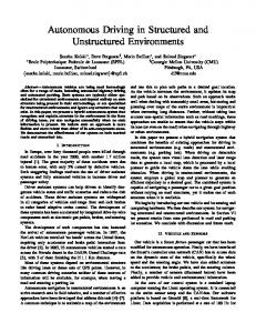
GOAL

START Fig. 1. Multi-level parking garage used for the experiment. The garage has four levels. The start point was close to the entrance, the goal point is on the upper level.

in large-scale indoor structures such as the one depicted in Fig. 1, which is the parking garage used for the experiments carried out for the work described in this paper. To enable a mobile vehicle to park itself at an arbitrary, pre-defined position in that garage given it starts at the entrance of the building at the lowest level, several requirements need to be met. First, the vehicle needs an appropriate representation of the building to calculate the path to be taken. Second, it needs to be able to localize itself in this three-dimensional building. Third, it needs to be able to follow this path so that it safely arrives at the designated target location. Our approach utilizes multi-level surface maps to compactly represent such buildings. We apply a graph-based optimization procedure to establish the consistency of this map. The map is then used to plan a global path from the start to the goal position and to robustly localize the vehicle based on laser range measurements. We use a local planner to follow this path and to avoid unforeseen obstacles. As a result, the vehicle can autonomously navigate in such multi-level environments without any additional information provided by a user. Our approach has been implemented and tested with a real Volkswagen Passat Wagon. The remainder of this paper is organized as follows. After discussing related work in the next section, we describe the underlying map data structure and the mapping algorithm in Section III. Our localization approach is presented in Section IV. In Section V we describe the planning algorithm. Finally, in Section VI, we present experimental results illustrating the abilities and advantages of our approach. II. R ELATED W ORK The system described in this paper addresses several aspects of autonomous robots including localization, mapping, path planning, and autonomous navigation. Several authors have studied the problem of mobile robot localization in outdoor environments with range sensors or cameras in the past. For example, Adams et al. [1] extract predefined

features from range scanners and apply a particle filter for localization. Davison and Kita [6] utilize a Kalman filter for vision-based localization with point features on non-flat surfaces. Agrawal and Konolige [2] presented an approach to robot localization in outdoor terrains based on feature points that are tracked across frames in stereo images. Lingemann et al. [19] described a method for fast localization in in- and outdoor environments. Their system operates on raw data sets, which results in huge memory requirements. Recently, Levinson et al. [17] presented an algorithm for mapping and localization in large urban environments. Their approach localizes the vehicle using 2D intensity images of the road surface which are obtained by the reflectivity measurements of a range scanner. Building maps of outdoor environments using range or vision data also gained interest in recent years. To reduce the memory requirements of outdoor terrain representations, several researchers applied elevation maps [3], [11], [15], [24]. This representation only stores one height value per cell which represents the drivable surface but is not sufficient to represent vertical or overhanging objects. Therefore, Pfaff et al. [25] extended elevation maps to also deal with vertical and overhanging objects. To also address the issue of multiple levels in the environment, e.g., a bridge and the corresponding underpass, Triebel et al. [28] presented multi-level surface (MLS) maps. The literature on path planning for wheeled robots is also extensive. Our local planner builds on the existing work in discrete search in unknown environments (e.g., [13], [8], [21]), as well as kinematic forward search [12], [16], [26] and nonlinear optimization in the space of 2D curves [4]. Whereas strategies for specific dedicated parking maneuvers have been developed [22], [23] and nowadays are even available in off-the-shelf vehicles, these systems perform autonomous navigation only in a short range and are not able to plan complex navigation tasks through entire parking structures. The work probably most closely related to ours is that of Schanz et al. [27] who developed an autonomous parking system in a subterranean parking structure. Compared to our work described in this paper, their system can only deal with given two-dimensional map representations and lacks the capability to detect obstacles in 3D. Additionally, their system cannot deal with multiple levels or drive on non-flat surfaces like ramps. III. M APPING OF THE PARKING G ARAGE A. Map Representation To model the environment, we apply MLS maps [28], which store the structure of the environment in a 2D grid of cells, where each cell cij , i, j ∈ Z contains a list of so-called surface patches Pij1 , . . . , PijL . For each patch, we store its height estimate µlij so that one can easily calculate the possibility to traverse the cell at a specific height. Additionally, we store for each patch the variance σijl to represent the uncertainty in the height of the surface. Furthermore, we represent a depth value to model the vertical extend of each patch. Fig. 2 depicts a local MLS-map close to one of the entrances of the parking garage used to

Fig. 2. Local MLS-map example. MLS-maps allows us to efficiently represent the drivable surface and the vertical objects, that are useful for localization.

carry out the experiments described in this paper. The local map consists of 15 point clouds. The MLS data structure allows us to represent complex outdoor environments in a compact manner. For example, the data set shown in the experiments consists of approximately 4 GB of raw data, while the complete MLS-map with a cell size of 20 cm requires only 128 MB. This amount of data easily fits into the main memory of modern computers and could in practical applications easily be downloaded to the navigation system of the car from the information system of the garage. B. Mapping with GraphSLAM Our mapping system addresses the SLAM problem by its graph-based formulation. A node of the graph represents a 6DoF pose of the vehicle and an edge between two nodes models a spatial constraint between them. These spatial constraints arise either from overlapping observations or from odometry measurements. In our case the edges are labeled with the relative motion between two nodes which determine the best overlapping between the 3D scans acquired at the nodes locations. To compute the spatial configuration of the nodes which best satisfies the constraints encoded in the edges of the graph, we use an online variant of a stochastic gradient optimization approach [9]. Performing this optimization procedure allows us to reduce the uncertainty in the pose estimate of the robot whenever constraints between nonsequential nodes are added. The graph is constructed as follows: whenever a new observation zt has to be incorporated into the system, we create a new node in the graph at position xt = (x, y, z, ϕ, ϑ, ψ). We then create a new edge et−1,t between the current position xt and the previous one xt−1 . This edge is then labeled with the transformation between the two poses xt ⊖xt−1 . We determine the position of the current node with respect to the previous one by 3D scan-matching. To this end, we use an approach based on the iterative closest points (ICP) algorithm to obtain a maximum likelihood estimate of the robot motion between subsequent observations. In our implementation we perform ICP on local MLS-maps instead of raw 3D point clouds. Whereas this procedure significantly improves the estimate of the trajectory, the error of the current robot pose tends to increase due to the accumulation of small residual errors. This effect becomes visible when the vehicle revisits already

known regions. To solve this problem, we need to re-localize the robot in a region of the environment which has been visited long before. To resolve these errors, (i.e., to close the loop), we apply our scan matching technique on our current pose xt and a former pose xi , whereas i ≪ t. To detect a potential loop closure, we identify all former poses which are within a constant error ellipsoid and whose observations overlap with the current observation. If a match is found, we augment the graph by adding a new edge between xi and xt labeled with the relative transformation between the two poses computed by matching their corresponding observations. This procedure works well as long as the relative error between the two poses lies within the error ellipsoid. In general, the longer the path between the two nodes xt and xi is, the higher the relative error becomes so that our simple strategy might fail. In the absence of a globally consistent position estimate like GPS to restrict the search of loop closures one might use more sophisticated techniques [5], [10]. While we acknowledge this drawback, during our experiments our strategy never introduced a wrong constraint and the resulting map was always consistent. C. Level Information As mentioned above, the MLS-map stores information about the surface which encloses the occupied volume of the environment. We can exploit this fact to assign progressive IDs to the different drivable levels in the map. We refer to a multi-level environment, if the robot has the possibility to reach a specific cell cij at least at two different height levels. To label the environment, we proceed as follows: First we generate a connectivity graph G of the surface described by the MLS map. This is done by connecting all the patches Pij1 , . . . , PijL of the cell cij with their neighboring patches of the cells {ci+k ,j +l | k, l ∈ {0, 1}, k + l ≥ 1} with an undirected edge. The edge is only introduced, if the height difference between the two surface patches is below a threshold. The step threshold is given by the characteristics of the robot. This connectivity graph is then used to initiate a region growing procedure. The initial frontier consists of the lowest surface patch. We keep the frontier sorted according to the surface height. The algorithm keeps track on how often each cell has been visited at different height levels. This counter is incremented whenever the cell is reached. In case the counter of the current cell is less than the counter of the predecessor, we set it to the level counter of the predecessor. In our approach, the level information is needed for the update of local two-dimensional data structures of our system. Whenever the car moves to a different level, we need to recompute these structures according to the current level. An example of a two-dimensional data structure which needs to be updated upon a change of the level is the twodimensional obstacle map. IV. L OCALIZATION Whenever the GPS signal is lost, even high-end integrated navigation units which combine GPS, wheel odometry via

a distance measurement unit, and inertial measurements to obtain a global position expressed in latitude, longitude, and altitude are not able to accurately localize the robot. In this case, the lack of GPS measurements prevents the system to compensate for the drift in the (x, y, z) position. This drift results from the integration of small errors affecting the relative measurements obtained by the encoders and the inertial sensors. In particular, we observed a significant error along the z component of the pose vector, which represents the height of the vehicle. This high error does not allow us to directly use the z estimate of the inertial system to estimate the level in case of multi-level indoor environments. To this end, we extended our former localization approach [14] which utilizes a particle filter to localize the car within a 3D map of the environment. The inertial navigation system integrates velocities and wheel odometry to calculate the position of the vehicle. This gives a locally consistent estimate, which is updated at 200 Hz. In addition we observed that the orientation, namely the roll, pitch, and yaw angles, is measured with high precision and also drift-free by the system. We also found, that the pose estimate is not significantly improved by filtering the attitude. Hence, we reduce the localization problem to three dimensions instead of six. Let xt = (x, y, z)T denote the pose of the particle filter at time t. The prediction model p(xt | ut−1 , xt−1 ) is implemented by drawing a 3D motion vector out of a Gaussian whose mean ut−1 is given by the relative 3D motion vector of the inertial system since time step t − 1. In addition, we constraint the height coordinate z of each particle to remain in a boundary around the surface modeled in the map. This is motivated by the fact, that positions above or below the surface are not admissible and we want to focus the limited number of particles in the high density regions of the probability density function. In all our experiments this boundary was set to 20 cm around the drivable surface. The range measurement zt is integrated to calculate a new weight for each particle according to the sensor model p(zt | xt ). The sensor model is implemented as described in our previous work [14]. Furthermore, the particle set needs to be re-sampled according to the assigned weights to obtain a good approximation of the pose distribution. We bootstrap our localization algorithm by initializing the particles based on the GPS measurements. Therefore, the map of the environment also contains the surrounding outdoor area where the GPS signal is available. In the outdoor part of the map, GPS provides a sufficiently accurate pose estimate to initialize the particle filter for position tracking. V. PATH P LANNING Given a search space, in our case the surface connectivity graph G described in Section III-C, we want to find a feasible path between a starting and a goal location. By defining a cost function for each motion command the robot can execute, and an admissible heuristic which efficiently guides the search, we can use A∗ to efficiently search for the path.

Velodyne laser Riegl laser

Sick LMS IMU GPS

LD−LRS Ibeo laser

Fig. 3. Local planner. The red curve is the trajectory produced by phase one of our search (local-A∗ ). The blue curve is the final smoothed trajectory produced by conjugate-gradient optimization.

Given a global path through the multi-level graph G, we use a local planner to navigate through the current level of the structure. The local planner uses the 2D obstacle map generated in real-time for the current level. Our local planner is based on the path planner used in the DARPA Urban Challenge by the Stanford racing team [7]. For completeness, we briefly outline the main components of this planner below. The task of the local planner is to find a safe, kinematically feasible, near-optimal in length, and smooth trajectory across the current 2D level of the environment. Given the continuous control set of the robot, this yields a complex optimization problem in continuous variables. For computational reasons, the local planner breaks the optimization into two phases. The first phase performs an A∗ search on the 4dimensional state space of the robot hx, y, θ, di, where hx, y, θi define the 2D position and orientation of the vehicle and d = {0, 1} corresponds to the direction of motion (forward or backwards). A∗ uses a heuristic that combines two components. The first component models the nonholonomic nature of the car, but ignores the current obstacle map. This heuristic—which can be pre-computed offline— ensures that the search approaches the goal with the right heading θ. The second component of the heuristic is dual to the first one in that it ignores the non-holonomic nature of the vehicle, but takes into account the current obstacle map. Both components are admissible in the A∗ sense, so we define our heuristic as the maximum of the two. The output of the first phase using the (A∗ ) search yields a safe and kinematicallyfeasible trajectory. However, for computational reasons we can only use a highly-discretized set of control actions in the search, which leads to sub-optimal paths. The second phase of local planning improves the quality of the trajectory via numerical optimization in continuous coordinates. We apply a conjugate-gradient (CG) descent algorithm to the coordinates of the vertices of the path produced by A∗ to quickly obtain a locally optimal solution. Our optimization uses a carefully constructed potential function defined over 2D curves (see [7] for more details) to produce a locally optimal trajectory that retains safety and kinematic feasibility. In practice, the first phase (A∗ ) typically produces a solution that lies in the neighborhood of the global optimum, which means that our second phase (CG) then produces a solution that is not only locally, but globally optimal.

DMI

Fig. 4. The car used for the experiment is equipped with five different laser measurement systems and a multi-signal inertial navigation system.

An example trajectory generated by the local planner is shown in Fig. 3. The red curve shows the output of phase one (A∗ ); the blue curve shows the final smooth trajectory produced by CG. In summary, our path planning uses a global planner operating on the topological graph G to produce a global path through the multi-level structure. The global planner iteratively calls a local planner to find a safe, feasible, and smooth trajectory through the current 2D level of the environment. VI. E XPERIMENTS Our approach has been implemented and evaluated on a modified 2006 Volkswagen Passat Wagon (see Fig. 4), equipped with multiple laser range finders (manufactured by IBEO, Riegl, Sick, and Velodyne), an Applanix GPSaided inertial navigation system, five BOSCH radars, two Intel quad core computer systems, and a custom drive-bywire interface. The automobile is equipped with an electromechanical power steering, an electronic brake booster, electronic throttle, gear shifter, parking brake, and turn signals. A custom interface-board provides computer control over each of these vehicle elements. For inertial navigation, an Applanix POS LV 420 system provides real-time integration of multiple dual-frequency GPS receivers which includes a GPS Azimuth Heading measurement subsystem, a high-performance inertial measurement unit, wheel odometry via a distance measurement unit (DMI), and the Omnistar satellite-based Virtual Base Station service. The real-time position and orientation errors of this system were typically below 100 cm and 0.1 degrees, respectively. Although the car is equipped with multiple sensor systems only data from the Velodyne LIDAR and the two side mounted LD-LRS lasers were used for the experiment. The Velodyne HDL-64E is the primary sensor for obstacle detection. The Velodyne laser has a spinning unit that includes 64 lasers which are mounted on upper and lower blocks of 32 lasers each. The system has a 26.8 degree vertical FOV and a 360 degree FOV collecting approximately 1 million data points each second. The spinning rate in our setup is 10 Hz which means that one full spin includes approximately 100,000 points. The maximum range of the sensor is about 60 m. Due to the high mounting of the sensor and the shape of the car, areas close to the car are occluded. We use two additional LD-LRS laser scanners to cover this area.

Fig. 5. Necessary steps for the 2d map building. First, the sensor measurements from the Velodyne laser (left image) are analyzed for obstacles. The obstacle measurements are discretized in 15 cm grid cells (red cubes in the middle image). These cells are used to generate a virtual 2D scan (right image) for updating a two-dimensional map. Yellow beams indicate that no obstacle is measured in this direction and a fixed range is used for the update. The two-dimensional map is used for the low level parking planner.

The software utilized in this experiment is based on the system used in the DARPA Urban Challenge. The architecture includes multiple modules for different tasks in the system like communication to the hardware, obstacle detection, 2D map generation, etc. [20]. Here, we focus on the modules relevant for the experiment. First, there is the low level controller that executes a given trajectory. The speed is based on the curvature of the trajectory and the maximum speed was set to 10 km/h. Second, there is the local planner described in Section V. Additionally an obstacle detection module analyzes the sensor data (see Fig. 5 (left)), discretizes the found obstacles points in a fixed sized (2D) grid (see Fig. 5 (middle)), and builds a 2D grid map. It generates a virtual 2D scan from the obstacle data (see Fig. 5 (right)) to update the map. The resulting map is then used by the local planner to generate the trajectory. The localization described in Section IV sends translational correction parameter to the other modules to compute the correct position. Finally, there is the global path planner that computes a full trajectory on the surface map to the goal point using A∗ . The global path is then divided into sub-goals. The program watches the progress of the car and updates the sub-goal to keep a fixed distance of approximately 20 m to the car. This way, the global path planner leads the car along the computed trajectory and allows the local planner to avoid local obstacles like parked cars that are not included in the map. We did three different experiments to show the functionality of the system. First we demonstrate that we can build a MLS-map from collected sensor data of the parking garage. Second we illustrate that the described localization technique is essential for our experimental setup, and finally we show that based on our implementation, a car can autonomously drive and park in a multi-level parking structure. A. Mapping To obtain the data set, we steered the robot along a 7,050 m long trajectory through the parking garage and the surrounding environment. The trajectory contains multiple nested loops on different levels of the garage. The robot collected more than 15,000 3D point clouds by its Velodyne sensor. This data has been merged into 1,660 local MLSmaps used for scan matching to learn the map. The outcome of our SLAM algorithm can be seen in Fig. 6. The cell size of the generated map was set to 20 cm. The parking garage

Fig. 6. The MLS map used for the experiment. The trajectory of the robot as it is estimated by the SLAM system is drawn in blue.

Fig. 7. Bird’s eye view of the parking garage. The red trajectory shows the position as it is estimated by the inertial navigation system, whereas the blue trajectory is estimated using our localization approach.

used for the experiments consists of four levels and covers an area of approximately 113 m by 100 m. B. Localization The described localization algorithm was evaluated on several separate data sets, that have been acquired at different points in time. Hence, the environment was subject to change, i.e., parked cars sensed during map building are no longer present. In all our experiments the particle filter was able to accurately localize the vehicle in real-time. The algorithm is able to perform pose correction with the update rate of the sensors using 1,000 particles, whereas the proposal distribution is updated at 200 Hz. Fig. 7 depicts the outcome of the localization algorithm. Note the trajectory as it is estimated by the inertial navigation system contains large errors, while driving without GPS coverage. Actually, the estimated trajectory is outside the boundaries of the parking garage after the car reached the third level. Not until the car reaches the top level and again receives GPS fixes, it is able to reduce this error. In contrast to this, our localization algorithm using the MLS-map and the range measurements

15 10 5 0 -5 -60 -40 -20

0

20

200 160 120

Fig. 8. Trajectory of the autonomous driving inside the parking structure. The left image shows the complete trajectory from the start point in the first level to goal point in the fourth level. The right image shows the last part of the trajectory to the goal point behind an obstacle (lamp pole).

is able to accurately localize the vehicle all the time. The accuracy of our localization is confirmed by the inertial navigation system whenever it receives valid GPS fixes, as the trajectories overlay at that time. C. Autonomous Driving The following experiment is designed to show the abilities of our approach to autonomously drive in a multi-level parking garage. The task of the vehicle was to drive from the start position, which was close to the entrance, to a parking spot on the upper level of the parking garage. Fig. 1 depicts an aerial image of the parking garage, in which the start and goal have been marked. The car autonomously traveled to the target location. The resulting 3D trajectory of the vehicle is depicted in Fig. 8 (left). The trajectory has a total length of 375 m and it took 3:26 minutes to reach the goal with an average speed of 6.6 km/h (maximum speed 9.5 km/h). Fig. 8 (right) depicts the trajectory of the local planner to the goal. VII. C ONCLUSIONS In this paper, we presented a novel approach for autonomous driving in complex GPS-disabled multi-level structures with an autonomous car. We described the individual approaches for mapping, SLAM, localization, path planning, and navigation. Our approach has been implemented and evaluated with a real Volkswagen Passat Wagon in a large-scale parking garage. The experimental results demonstrate that our approach allows the robotic car to drive autonomously in such environments. The experiments furthermore illustrate, that a localization algorithm is needed to operate indoors, also in the case in which the robot is equipped with a state-of-the-art combined inertial navigation system. R EFERENCES [1] M. Adams, S. Zhang, and L. Xie. Particle filter based outdoor robot localization using natural features extracted from laser scanners. In Proc. of the IEEE Int. Conf. on Robotics & Automation (ICRA), 2004. [2] M. Agrawal and K. Konolige. Real-time localization in outdoor environments using stereo vision and inexpensive gps. In International Conference on Pattern Recognition (ICPR), 2006. [3] J. Bares, M. Hebert, T. Kanade, E. Krotkov, T. Mitchell, R. Simmons, and W. R. L. Whittaker. Ambler: An autonomous rover for planetary exploration. IEEE Computer Society Press, 22(6):18–22, 1989. [4] L.B. Cremean, T.B. Foote, J.H. Gillula, G.H. Hines, D. Kogan, K.L. Kriechbaum, J.C. Lamb, J. Leibs, L. Lindzey, C.E. Rasmussen, A.D. Stewart, J.W. Burdick, and R.M. Murray. Alice: An information-rich autonomous vehicle for high-speed desert navigation. Journal of Field Robotics, 2006. Submitted for publication. [5] M. Cummins and P. Newman. Probabilistic appearance based navigation and loop closing. In Proc. IEEE International Conference on Robotics and Automation (ICRA’07), Rome, April 2007.

[6] A Davison and N. Kita. 3D simultaneous localisation and mapbuilding using active vision for a robot moving on undulating terrain. In Proc. IEEE Conference on Computer Vision and Pattern Recognition, Kauai. IEEE Computer Society Press, December 2001. [7] D. Dolgov, S. Thrun, M. Montemerlo, and J. Diebel. Path planning for autonomous driving in unknown environments. In Proceedings of the Eleventh International Symposium on Experimental Robotics (ISER-08), Athens, Greece, July 2008. [8] D. Ferguson and A. Stentz. Field d*: An interpolation-based path planner and replanner. In Proc. of the International Symposium of Robotics Research (ISRR), 2005. [9] G. Grisetti, D. Lodi Rizzini, C. Stachniss, E. Olson, and W. Burgard. Online constraint network optimization for efficient maximum likelihood map learning. In Proc. of the IEEE Int. Conf. on Robotics & Automation (ICRA), Pasadena, CA, USA, 2008. [10] D. H¨ahnel, W. Burgard, B. Wegbreit, and S. Thrun. Towards lazy data association in SLAM. In Proc. of the International Symposium of Robotics Research (ISRR), Siena, Italy, 2003. [11] M. Hebert, C. Caillas, E. Krotkov, I.S. Kweon, and T. Kanade. Terrain mapping for a roving planetary explorer. In Proc. of the IEEE Int. Conf. on Robotics & Automation (ICRA), pages 997–1002, 1989. [12] L. Kavraki, P. Svestka, J. C. Latombe, and M. Overmars. Probabilistic road maps for path planning in high-dimensional configuration spaces. IEEE Transactions on Robotics and Automation, pages 566–580, 1996. [13] S. Koenig and M. Likhachev. Improved fast replanning for robot navigation in unknown terrain. In Proc. of the IEEE Int. Conf. on Robotics & Automation (ICRA), 2002. [14] R. K¨ummerle, R. Triebel, P. Pfaff, and W. Burgard. Monte carlo localization in outdoor terrains using multilevel surface maps. Journal of Field Robotics (JFR), 25:346–359, June - July 2008. [15] S. Lacroix, A. Mallet, D. Bonnafous, G. Bauzil, S. Fleury, M. Herrb, and R. Chatila. Autonomous rover navigation on unknown terrains: Functions and integration. International Journal of Robotics Research, 21(10-11):917–942, 2002. [16] S. LaValle. Rapidly-exploring random trees: A new tool for path planning. Technical Report TR 98-11, Computer Science Dept., Iowa State University, 1998. [17] J. Levinson, M. Montemerlo, and S. Thrun. Map-based precision vehicle localization in urban environments. In Proceedings of Robotics: Science and Systems, Atlanta, GA, USA, June 2007. [18] M. Likhachev and D. Ferguson. Planning long dynamically-feasible maneuvers for autonomous vehicles. In Proceedings of Robotics: Science and Systems IV, Zurich, Switzerland, June 2008. [19] K. Lingemann, H. Surmann, A. N¨uchter, and J. Hertzberg. Highspeed laser localization for mobile robots. Journal of Robotics & Autonomous Systems, 51(4):275–296, 2005. [20] M. Montemerlo et al. Junior: The Stanford entry in the urban challenge. Journal of Field Robotics, 25(9):569–597, 2008. [21] A. Nash, K. Daniel, S. Koenig, and A. Felner. Theta*: Any-angle path planning on grids. In Proc. of the National Conference on Artificial Intelligence (AAAI), pages 1177–1183, 2007. [22] I.E. Paromtchik and C. Laugier. Autonomous parallel parking of a nonholonomic vehicle. In Proc. of the IEEE Intelligent Vehicles Symposium, 1996. [23] I.E. Paromtchik and C. Laugier. Automatic parallel parking and returning to traffic maneuvers. In Proc. of the IEEE/RSJ Int. Conf. on Intelligent Robots and Systems (IROS), volume 3, pages V21–V23, 1997. [24] C. Parra, R. Murrieta-Cid, M. Devy, and M. Briot. 3-D modelling and robot localization from visual and range data in natural scenes. In 1st International Conference on Computer Vision Systems (ICVS), number 1542 in LNCS, pages 450–468, 1999. [25] P. Pfaff, R. Triebel, and W. Burgard. An efficient extension to elevation maps for outdoor terrain mapping and loop closing. International Journal of Robotics Research, 26(2):217–230, 2007. [26] E. Plaku, L. Kavraki, and M. Vardi. Discrete search leading continuous exploration for kinodynamic motion planning. In Robotics: Science and Systems, June 2007. [27] A. Schanz, A. Spieker, and K.-D. Kuhnert. Autonomous parking in subterranean garages-a look at the position estimation. In Proc. of the IEEE Intelligent Vehicles Symposium, 2003. [28] R. Triebel, P. Pfaff, and W. Burgard. Multi level surface maps for outdoor terrain mapping and loop closing. In Proc. of the IEEE/RSJ Int. Conf. on Intelligent Robots and Systems (IROS), 2006.