Towards Autonomous Driving in a Parking Garage: Vehicle Localization and Tracking Using environment-embedded LIDAR Sensors Andr´e Ibisch∗ , Stefan St¨umper◦ , Harald Altinger◦ , Marcel Neuhausen∗ , Marc Tschentscher∗ , Marc Schlipsing∗ , Jan Salmen∗ , and Alois Knoll• Abstract— In this paper, we propose a new approach for localization and tracking of a vehicle in a parking garage, based on environment-embedded LIDAR sensors. In particular, we present an integration of data from multiple sensors, allowing to track vehicles in a common, parking garage coordinate system. In order to perform detection and tracking in realtime, a combination of appropriate methods, namely a gridbased approach, a RANSAC algorithm, and a Kalman filter is proposed and evaluated. The system achieves highly confident and exact vehicle positioning. In the context of a larger framework, our approach was used as a reference system to enable autonomous driving within a parking garage. In our experiments, we showed that the proposed algorithm allows a precise vehicle localization and tracking. Our system’s results were compared to human-labeled ground-truth data. Based on this comparison we prove a high accuracy with a mean lateral and longitudinal error of 6.3 cm and 8.5 cm, respectively.
I. I NTRODUCTION In the last decades, many different technical approaches have been realized to increase drivers’ safety and comfort. The combination of accurate sensors and powerful algorithms led to Advanced Driver Assistance Systems (ADAS), which are able to support the driver in critical situations (e.g., lane departure warning) or relieve him by autonomously performing exhausting maneuvers (e.g., parking assistance). As a consequence, vehicles will drive fully autonomous in the long term. Nowadays, this kind of autonomy is only realizable within restricted scenarios. In this study, we present a new approach for localization and tracking of vehicles within known environments using the example of parking garages. Our approach is particularly interesting, because many people feel uncomfortable in such environments for different reasons: • Driving in narrow buildings with sometimes confusing architecture is stressful. • The elderly or disabled people encounter problems entering their car in narrow parking spots [1]. • People feel unsafe. ∗ Institut f¨ ur Neuroinformatik, Ruhr-Universit¨at Bochum, Germany. {andre.ibisch, marcel.neuhausen, marc-philipp.tschentscher, marc.schlipsing, jan.salmen}@ini.rub.de ◦ AUDI AG, Ingolstadt, Germany. {stefan.stuemper, harald.altinger}@audi.de • Institut f¨ ur Informatik VI, Technical University Munich, Germany.
[email protected]
Finding a free parking spot is time-consuming and tedious. In this paper, we present an environment-embedded method for localization and tracking of vehicles in a parking garage based on LIDAR (Light detection and ranging) sensors. In the context of a parking assistance system those results and additional vehicle sensory data is used to realize autonomous driving. Within that major system the driver hands over his car at the parking garage entrance. The vehicle is then driven autonomously through the building towards a free parking spot and can be picked up later similarly. The proposed localization system gathers reliable data for various indoor scenario where GPS information is not available. It is flexible and extendible as it is able to cover different sizes of vehicles (e.g., trucks or robots) in huge indoor areas. In order to achieve these goals we base our system on multiple LIDAR sensors embedded in the parking garage environment. LIDAR sensors measure distances with a high accuracy and a fast sampling rate. This paper will firstly give an overview of related work in Sec. II. The proposed approach is presented in Sec. III. In Sec. IV the implemented system is tested and evaluated in a parking garage. A final conclusion and outlook is given in Sec. V. •
II. R ELATED WORK LIDAR sensors mounted on moving objects have been widely used for detection and tracking of relevant objects [1] [2] as well as for self-positioning [3] in different fields of application (robotics, automotive, etc.) or to gather information about unknown environments. Here, we focus on applications in the context of parking scenarios. In [1], Supp´e et al. presented an approach to assisted parking using LIDAR sensors attached to the vehicle and odometry information. Their system allows the driver to operate his vehicle by observing its trajectory with a remote control from outside the car. K¨ummerle et al. introduce an approach for autonomous parking in absence of GPS data in a parking garage [2]. Although their system is very accurate with a position error of 0.1 m, it is not suitable for common vehicles, as five different laser systems and five radar sensors are mounted on the test carrier. In contrast to that, we employ stationary environmentembedded sensors within the infrastructure. The proposed
(a) Position of the LIDAR sensor on (b) Typical parking garage scenario. the parking garage.
The following sections are structured analog to the above described processing chain. The sensor network employed for our system is described in Sec. III-A. Section III-B illustrates the separation of active points applied to each sensor. A one-time calibration for combining sensors into a shared world coordinate system is specified in Sec. III-C. The methods for detecting and tracking vehicles are described in Sec. III-D and III-E, respectively. A. Sensor network
(c) LIDAR data of the recorded setting. Fig. 1. A typical parking garage scenario of our system: (a) shows a single LIDAR sensor in the parking garage aligned to measure in parallel to the ground plane. The LIDAR sensor in this picture is positioned behind the vehicle. (b) displays the same scenario from an different point of view. (c) presents the bird’s-eye-view of the captured LIDAR data in this scenario. The blue box marks the sensor position. The four measurement clusters above-right of the sensor correspond to the vehicle’s wheels.
A LIDAR sensor measures distances between the sensor and its environment by using a set of laser rays. The sensor emits a laser pulse, detects the light reflected by an object and deduces its distance from the time of flight. For the proposed system, several LIDARs are connected in a sensor network in order to cover the relevant plane of the parking garage. The result of a single measurement step is a set of 2D points (x, y) represented in a sensor centered coordinate system. In order to cover the relevant section of the observed scene, a comprehensive calibration of the sensor network is necessary. It is noteworthy that measuring is performed in a single fixed 2D plane. We adjust all LIDAR sensors in the parking garage near the floor and parallel to the ground plane. This setup allows to measure points on the wheels and perform detection based on this information (see Sec. III-D). B. Active points
approach is cost efficient, does not require vehicles with specific equipment and is, therefore, easily transferable to real-world scenarios. Another system for autonomous driving in a parking garage using a network of video cameras is discussed in [4]. The authors observed an aberration in their predicted vehicle hypotheses of 1 m with a coverage of 14 m due to the cameras extrinsic constraints. III. P ROPOSED SYSTEM The proposed system is based on LIDAR data only and aims at the estimation of the vehicles’ position and orientation in coordinates of a parking garage. To achieve applicability, the system should be failsafe, accurate, and real-time capable. A typical parking garage scenario with the corresponding LIDAR data measurements is illustrated in Fig. 1. The presented approach is structured in a feed forward manner: Each single sensor records data points from its environment. Then, measurements are separated into static and active (i.e., moving) points using (see Sec. III-B) temporal filtering. Active points of each sensor are transformed into a common world coordinate system. This representation allows to employ detection algorithms on combined sensor data for generating feasible vehicle hypotheses. Finally, hypotheses for single frames are tracked to ensure stable and distinct vehicle positioning.
A large set of LIDAR measurements originate from static objects, e.g., walls. In order to increase robustness and computational efficiency of our approach, we aim at processing only a small subset of active points. To separate task-relevant from non-relevant points, we propose a 2D grid-based approach in combination with an initial learning phase. The grid consists of quadratic cells, covering the area in front of a LIDAR sensor with the specific parameters (width, height, cell resolution), the angle resolution and the maximum detection range of the sensor. A single cell is defined by its center (x, y) and radius r, defining a search area (πr2 ) for corresponding rays. It captures all passing rays Rcell = {r0 , r1 , . . . , rn } and categorizes them by their length |ri |, which is the distance of the measurement to the sensor. To estimate the probability of a cell being idle, rays are divided into measurements that lie behind the cell boundaries Rfar and those ending in front the cell Rbefore . Rays which hit the cell are not explicitly regarded, as they imply occupancy. o n p (1) Rfar = ri ∈ Rcell | x2 + y 2 − r ≤ |ri | ,
n o p Rbefore = ri ∈ Rcell | x2 + y 2 + r ≥ |ri | ,
pcell =
|Rfar | |Rbefore | + 0.5 · |R| |R|
(2)
(3)
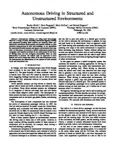
(a) CAD representation
(b) LIDAR Data
Fig. 3. CAD representation of a parking garage and a set of LIDAR measurements produced by three sensors. Fig. 2. A grid representation (20 m × 10 m) of the scenario from Fig. 1: The grid subdivides the LIDAR sensor measurements into active and static points. The cell probabilities are visualized with different colors. An occupied cell is drawn with red, an uncertain cell with yellow and a free cell is painted with green.
ptcell = pt−1 cell + α · pcell
(4)
Probability pcell represents the level of the occupation of the cell in a single time frame, where 1 means free, 0 indicates occupied and 0.5 uncertain. The overall probability ptcell of a cell considering consecutive measurements is exponentially smoothed with rate α in order to stabilize a reliable grid representation. Figure 2 shows the result of the learning phase. Given a threshold for the cell occupancy, one is now able to assign each measurement based on the occupancy value of its corresponding learned cell to decide whether it is active or static. To speed up the calculation we propose a preprocessing. Instead of calculating each relevant cell of a LIDAR ray in each time step, a precalculation step of the grid calculates all regarded rays for each single cell. Thus, a cell compares only its stored rays with the currently measured rays. After this phase a second learning phase is launched. This phase enables continuous learning of a grid to adapt slower environment changes (e.g., changes of the occupation of a parking lot). Due to real-time constraints we cannot update every single cell in a time frame, because a sufficient grid contains up to 10,000 cells. For continuous learning a randomized subset of grid cells is updated. Therefore, every cell holds a ring buffer for each of the categories mentioned above. The ring buffer stores the last n rays according to its category and calculates a weighted sum for each category to determine the occupancy probability. The size of the ring buffer n affects the speed of learning. The background subtraction reduces the amount of data points to be processed by a factor of 10. C. Sensor Stitching After identifying active points in the LIDAR sensor separately, one has to avoid multiple detections of the same object and handle occlusions or intersections of moving objects across different sensors. This could lead to false negative detections, e.g., two detected wheels in two different sensors of one vehicle is not enough for a plausible detection (see Sec, III-D). The aggregation of different vehicle hypotheses
of a single sensor detection could also lead to false positive detections, caused eventually by contradicting information. Thus, we do not perform vehicle detection for all sensors separately, but propose a more generic approach: Active measurements are aggregated in one common representation, which is based on world coordinates of the given parking garage. To establish a shared coordinate system, a CAD map of the garage is used (see Fig. 3). Measured data of each sensor is transformed into this coordinate system using projective linear transformations (homography). Therefore, the direct linear transformation (DLT) algorithm [5] is employed, leading to a warp matrix on the basis of labeled correspondences (point to point or line to line).
(a) Frontal view.
(b) Opposite view.
(c) Stitched Result. Fig. 4. A LIDAR stitching result of two LIDAR sensors: (a) shows a single LIDAR sensor measurement. The vehicle is positioned frontal to the first sensor. (b) shows the data from the second LIDAR positioned on the opponent side. Finally in (c) both LIDAR sensors are combined in a world representation after the stitching process.
Two different kind of transformations are possible: A coordinate system of a LIDAR sensor transformed into another LIDAR coordinate system or to a specified repre-
sentation of the environment. The DLT requires at least four correspondences between sensor and map coordinates. To determine the correspondences, an operator calibrates the setup once. The operator marks the particular set of points or lines in both coordinate systems. For a good estimate of the warp matrix, these correspondences should to be widespread inside the environment and must not be collinear. A stitching result for a vehicle captured by two LIDAR sensors is shown in Fig. 4. An alternative calibration manipulates an identity matrix by executing several manual turning and translating operations until the LIDAR data adjusts to the representation. D. Detection After the active points are filtered (see Sec. III-B) and transformed by the sensor stitching (see Sec. III-C) the detection operates on a sparse subset of measurements. Because the sensors are deployed right above the ground plane (see Sec. III-A) these active points contain different moving objects: peoples’ feet can cross the sensor plane, miss-measurements due to noise, and the targeted vehicles. The detection should only find plausible and precise hypotheses and provide the vehicle’s center and orientation. Because vehicles have various appearances, e.g., form or height of the car body, the best traceable feature of a vehicle is the well-known shape of a wheel. The recognition of at least three wheels yields strong cues regarding the orientation of the car. To apply this knowledge to the LIDAR data we constructed an abstract and parameterized vehicle model. This model is based on a rectangular composition of four wheels with a certain tolerance (cf. Fig. 5). Two alternative and efficient approaches operating with this model have been realized: The Hough transformation (see [6]) observes two different measurements from active points, calculates their distance, builds up an appropriate vehicle hypothesis and performs a vote in the hough parameter space. An accumulation of hypotheses reasons to a plausible vehicle hypothesis. We also applied a RANSAC
(random sample consensus) algorithm [7] operating with this model. The RANSAC algorithm is a randomized method to eliminate outliers and consists of two phases, proof and evaluation. In the proof phase, randomized sets of three active points are drawn. These sets are tested against the rectangle of our vehicle model. In the evaluation phase, all hypotheses from the first phase are sorted by a confidence, considering the number of measurements that are reasonably close to each of the four points (wheels) and a minimum number of supported wheels. In the end, a set of hypotheses with sufficient confidence is chosen for the following tracking module. To improve tracking (see Sec. III-E), we also generate hypotheses based on only two active points. These hypotheses are ambiguous, because the two active points could either lie on a short / long edge or on the opposite site. Nevertheless, treated separately, those are helpful to update occluded tracks. E. Tracking The tracking module receives the hypotheses from the detection module and has to ensure a consistent and complete temporal integration by providing the filtered vehicle’s center and orientation. A comprehensive tracking assumes a gapless classification of vehicles, either based on a detected hypothesis, or a plausible prediction. This prediction closes gaps where no hypotheses are generated by the detection module. We suggest to employ an extended Kalman filter (e.g., see [8]) with a physical motion model and reasonable observation noise, because it is arguably the best-known temporal filter. We propose to manage the assignment of hypotheses to tracks as follows: The first time, an unobserved hypothesis appears, it initializes a new track. In the following steps, the most similar hypothesis concerning vehicle center and orientation updates the filter. A track is regarded stable after a certain number of these updates. If a track does not receive an hypothesis, the Kalman filter only predicts its new state. After a certain amount of predictions (without updates), the track is eliminated. Here, the alternative updates based on the two-point hypotheses of the RANSAC algorithm (see Sec. III-D) are conducted. Those are only considered for tracks which were not updated by three-point hypotheses. This procedure is useful to avoid the loss of a track where more than one wheel is occluded. Nevertheless, these hypotheses are not very reliable and, thus, are not used to initialize a new track. IV. E XPERIMENTS A. Setup
Fig. 5. A detected hypothesis (red rectangle) by the RANSAC algorithm and corresponding LIDAR measurements (blue dots).
We established an installation of six 2D SICK LIDAR LMS 500 distributed in a parking garage. These sensors allow to record up to 100 measurements per second at a minimal angular resolution of 1/6◦ in a field of view of up to 190◦ and a maximum operating distance of 65 m. All LIDAR sensors are part of a Local Area Network.
B. Results
34
y (in m)
32 30 28 26 24
10
20
25
30
35
40
Fig. 7. Trajectories of the vehicle’s center: GT data (blue) and estimated position (red). 10 5 0 −5 −10 0
100
200
300
400
500
600
500
600
time step difference in degree (in degree ◦ )
As a baseline for comparison, we developed two interchangeable detection algorithms (see Sec. III-D): The runtime interval of the Hough transformation varies between 25 ms and 50 ms. The RANSAC algorithm has a constant runtime of approx. 5 ms. There is only a minimally variation in runtime for sorting the initial hypotheses. Because of its real-time capability we only considered the results by our RANSAC algorithm. The quadratic runtime of the Hough transformation is caused by highly varying quantity of active points. The result of the runtime comparison is shown in Fig. 6.
15
x (in m)
difference in speed (in km/h)
Our parking garage consists of three different areas: An entrance area (30 m length × 15 m width), a ramp (35 m length × 6 m width) with a 8◦ fall and the parking area (30 m length × 15 m width). Each area is covered by two LIDAR sensors. Our experiments covered the main operations of a vehicle in a parking garage scenario: The analyzed sequence started with the acceleration of the vehicle on a ramp to the first parking floor. It drove within 30 seconds approx. 40 m straight ahead, slowed down, performed a left 90◦ turn and accelerated again in the parking area. To evaluate our system, we compared results with human labeled data. A human user assigned ground-truth (GT) position within unfiltered and raw recorded LIDAR data in every single time frame. In our sequence, approx. 600 hand-labeled GT positions containing the center and orientation of the vehicle were gathered. Because a tracker requires a certain number of consecutive initial detections, the evaluation was stated after this initial phase. Additionally the GT speed was calculated from sequenced positions, which is temporally smoothed to receive a stable estimate. The deployed system is a desktop PC with an Intel Core i7 CPU at 2.80 GHz and 4 GB RAM memory.
10 5 0 −5 −10 0
100
200
300
400
time step
runtime (in ms)
50
Fig. 8.
Difference in speed (top) and orientation (bottom).
40 30 20 10 0
0
100
200
300
400
500
600
time step
Fig. 6. Runtime analysis of the RANSAC algorithm (red) and Hough transformation (blue).
The trajectories of the GT data and the estimated data in coordinates of the parking garage are illustrated as a bird’s eye view in Fig. 7. The mentioned sequence starts near position (41, 33) and ends in the final position close to (8, 24). The driving direction within this plot is from right to left. The difference in speed (in km/h) between the
GT data and the prediction is shown in Fig. 8 (top) with a mean aberration of 0.82 km/h and a standard deviation of ±0.6 km/h. Figure 8 (bottom) displays the difference in orientation (in degree) between GT data and the orientation predicted by the Kalman filter. The mean absolute error was 1.07◦ with a standard deviation of ±1.16◦ . Figure 9 illustrates the lateral and the longitudinal error of the estimated position. The quality of the Kalman filter can be evaluated as follows: The predicted position inaccuracy of the orientation is extracted from the longitudinal and lateral error. The longitudinal error represents the aberration in driving direction (positive ahead) and the lateral error illustrates the sidewise aberration. The mean absolute lateral error amounts to 6.3 cm with a standard deviation of ±4.4 cm, and the mean absolute longitudinal error to 8.5 cm with a standard deviation of ±5.6 cm.
0.3
deviation (in m)
lateral error (in m)
0.2
0
−0.2 0
100
200
300
400
500
0.1
600 0
time step longitudinal error (in m)
0.2
0
100
200
300
400
500
600
time step
0.2
Fig. 10. Mean error of wheelIndex w, ¯ the predicted position regarding the wheels with respect to GT data. 0
−0.2 0
100
200
300
400
500
600
time step
Fig. 9. Lateral error (upper) and longitudinal error (lower) of the Kalman filter estimated position.
The mean euclidean distance between the vehicle center (GT and prediction) is 11.5 cm with a standard deviation of ±5.4 cm. To combine both, orientation and position, we proposed an index value by comparing the wheel positions of the GT data with the final predicted hypotheses on the basis of the orientation and the center of all four wheels. To ensure a reliable comparison we only match equivalent wheels with each other: P4 d(wGT (i), west (i)) w ¯ = i=1 , (5) 4 with the euclidean distance d(x, y) between two points x and y, wGT (m) representing the center of a wheel m of the hand labeled data, west (n) the analog wheel center of the calculated hypothesis with the index n. The result is shown in Fig. 10. The mean distance is 12.1 cm with a standard deviation of ± 5.1 cm. The mentioned errors are caused by the Kalman estimation by assigning initial detections to the present filter and are also smoothed in relation to past measurements. The gathering of GT data by a human user also induces some inaccuracy for the evaluation. Alternatively one could gain more accurate GT from differential GPS which was not available for our experiments. V. C ONCLUSION AND O UTLOOK In this paper we present a system for localization and tracking of vehicles in a parking garage scenario using a network of LIDAR sensors. Being part of a framework which enables autonomous driving, our system collects reliable positional data.
In the proposed processing chain we firstly subdivide a single measurement into active and static points to reduce complexity for further steps. This is realized by a precalculated grid coding free and occupied space. To obtain a world coordinate system, we described a semi-automatic sensor stitching with manual determination of correspondences in each coordinate system. To detect vehicles on these active and transformed points, we employed a RANSAC algorithm. The tracking module ensures temporal integration and handles the incoming vehicle hypotheses. In our experiments we showed, that our approach is a suitable localization reference system for a superordinate framework realizing autonomous driving inside a parking garage. The mean absolute lateral and longitudinal error of a tracked vehicle, compared to ground-truth, was evaluated as 6.3 cm and 8.5 cm, respectively. This LIDAR network system was integrated into a major system and was extended by vehicle mounted ultrasound sensors, cameras or vehicle odometry data. An advantage of our system in this parking garage scenario was the accuracy on wide lanes, while other sensors fail due to their limited range. R EFERENCES [1] A. Supp´e, L. Navarro, and A. Steinfeld, “Semi-autonomous virtual valet parking,” in Proceedings of the Second International Conference on Automotive User Interfaces and Interactive Vehicular Applications, 2010, pp. 139–145. [2] R. K¨ummerle, D. Hahnel, D. Dolgov, S. Thrun, and W. Burgard, “Autonomous driving in a multi-level parking structure,” pp. 3395– 3400, 2009. [3] C. Gao and J. Spletzer, “On-line calibration of multiple lidars on a mobile vehicle platform,” in Proceedings of the IEEE International Conference on Robotics and Automation, 2010, pp. 279–284. [4] J. Einsiedler, O. Sawade, B. Schaufele, M. Witzke, and I. Radusch, “Indoor micro navigation utilizing local infrastructure-base positioning,” in Proceedings of the IEEE Intelligent Vehicles Symposium, 2012, pp. 993–998. [5] R. I. Hartley and A. Zisserman, Multiple View Geometry in Computer Vision, 2nd ed. Cambridge University Press, 2004. [6] R. Gonzalez and R. Woods, Digital Image Processing. Prentice Hall, 2008. [7] M. Fischler and R.Bolles, “Random sample consensus: a paradigm for model fitting with applications to image analysis and automated cartography,” Communications of the ACM, vol. 24, no. 6, pp. 381– 395, 1981. [8] M. S. Grewal and A. P. Andrews, Kalman Filtering: Theory and Practice. Prentice-Hall, 1993.