Building Ensembles of Neural Networks with Class-switching Gonzalo Mart´ınez-Mu˜ noz, Aitor S´ anchez-Mart´ınez, Daniel Hern´ andez-Lobato and Alberto Su´ arez Universidad Aut´ onoma de Madrid, Avenida Francisco Tom´ as y Valiente, 11, Madrid 28049, Spain,
[email protected],
[email protected],
[email protected],
[email protected]
Abstract. We investigate the properties of ensembles of neural networks, in which each network in the ensemble is constructed using a perturbed version of the training data. The perturbation consists in switching the class labels of a subset of training examples selected at random. Experiments on several UCI and synthetic datasets show that these class-switching ensembles can obtain improvements in classification performance over both individual networks and bagging ensembles.
1
Introduction
Ensemble methods for automatic inductive learning aim at generating a collection of diverse classifiers whose decisions are combined to predict the class of new unlabeled examples. The goal is to generate from the same training data a collection of diverse predictors whose errors are uncorrelated. Ensembles built in this manner often exhibit significant performance improvements over a single predictor in many regression and classification problems. Ensemble can be built using different base classifiers: decision stumps [1] decision trees [2–5, 1, 6–10], neural networks [11–14, 9, 15], support vector machines [16], etc. Generally, ensemble methods introduce a random element somewhere in the process of generating of an individual predictor. This randomization can be introduced either in the algorithm that builds the base models or in the training datasets that these algorithms receive as input. The rationale behind injecting randomness into the base learning algorithm is that different executions of the randomized training algorithm on the same data should generate diverse classifiers. For example, in randomization [17] the base learners are decision trees generated with a modified tree construction algorithm. This algorithm computes the best 20 splits for every internal node and then chooses one at random. Another simple algorithm of this type consists in generating diverse neural networks using different random initializations of the synaptic weights. This simple technique is sufficient to generate fairly accurate ensembles [6].
The randomization of the training dataset can be introduced in different ways: Using bootstrap samples from the training data, modifying the empirical distribution of the data (either by resampling or reweighting examples), manipulating the input features or manipulating the output targets. Bagging [4], one of the most widespread methods for ensemble learning, belongs to this group of techniques. In bagging, each individual classifier is generated using a training set of the same size of the original training set, obtained by random resampling with replacement from it. In Boosting [2], the individual classifiers are sequentially built assigning at each iteration different weights to the training instances. Initially the weights of the training examples are all equal. At each iteration of the boosting process these weights are updated according to the classification given by the last generated classifier. The weights of correctly classified examples are decreased and the weights of incorrectly classified ones are increased. In this way the subsequent base learner focuses on examples that are harder to classify. Another strategy consists in manipulating the input features. For instance, one can randomly eliminate features of the input data before constructing each individual classifier. In random subspaces [18] each base learner is generated using a different random subset of the input features. Another data randomization strategy consists in modifying the class labels. In particular, in classification problems with multiple classes, one can build each classifier in the ensemble using a different coding of the class labels [19, 20]. Other algorithms that manipulate the output targets and that are not limited to multiclass problems are based on randomly switching the class label of a fraction of the training set to generate each classifier (e.g. flipping [21] and class-switching [22]). Class-switching ensembles composed of a sufficiently large number of unpruned decision trees exhibit a good generalization performance in many classification problems of interest [22]. In this article we analyze the performance of class-switching algorithm using neural networks as the base learners. Because of the different properties of neural networks and decision trees, several modifications of the procedure described in [22] need to be made to generate effective class-switching ensembles composed of neural networks. In Section 2, we introduce the class-switching algorithm based on modifying the class labels of the training examples and adapt it to build neural network ensembles. Section 3 presents experiments that compare the classification performance of a single neural network, class-switching and bagging ensembles in twelve datasets. Finally, the conclusions of this research are summarized in Section 4.
2
Class-switching Ensembles
Switching the class labels to generate ensemble of classifiers was first proposed by Breiman [21]. In this work we apply the class switching procedure as described in [22] using neural networks as base learners. Class-switching ensembles are built by generating each classifier in the ensemble using different perturbed versions of the original training set. To generate a perturbed version of the training set, a
fixed fraction p of the examples of the original training set are randomly selected and the class label of each of these selected examples is randomly switched to a different one. The class label randomization can be characterized by a transition probability matrix Pj←i = p/(K − 1) f or i 6= j (1) Pi←i = 1 − p , where Pj←i is the probability that an example whose label is i becomes labeled as belonging to class j. K is the number of classes in the problem. The class-flipping procedure proposed by Breiman [21] is designed to ensure that, on average, the class proportions of the original training set are maintained in the modified training sets. However, for class unbalanced datasets this procedure has proved not to perform efficiently [22]. On the contrary, classswitching ensembles [22] applied to decision trees has proved to be competitive with bagging and boosting ensembles for a large range of balanced and unbalanced classification tasks. In order for this method to work, the fraction of switched examples p, should be small enough to ensure that there are, for any given class, a majority of correctly labeled examples (i.e. not switched). This condition is fulfilled on the training set (on average) if Pj←i < Pi←i . Using (1) p < (K − 1)/K .
(2)
From this equation we define the ratio of the class-switching probability to its maximum value as pˆ = p/pmax = pK/(K − 1) . (3) Using values of p over this limit would generate, for some regions in feature space, a majority of examples incorrectly labeled and consequently those regions would be incorrectly classified by the ensemble. In Ref. [22] class-switching ensembles composed of unpruned decision trees were experimentally tested. Using unpruned decision trees instead of pruned trees was motivated by their better performance when combined in the ensemble. Note that, provided that there are no training examples with identical attributes values belonging to different classes, an unpruned decision tree achieves perfect classification (0 error rate) on the perturbed training set. Under these conditions and in order for class-switching to obtain good generalization errors it is necessary to combine a large number of trees in the ensemble (≈ 1000) and to use relatively high values of pˆ. Empirically a value of pˆ ≈ 3/5 produced excellent results in all the classification tasks investigated [22]. Preliminary experiments were performed to check whether the prescription used for decision trees (i.e. 0 training error of the trees on the perturbed sets, large number of units in the ensemble and high values of pˆ) can be directly applied to neural networks. Note that the architecture and training parameters of the neural network have to be tuned for each problem in order to obtain neural models with ≈ 0 error rates in the modified training sets. This is a drawback with respect to decision trees, where achieving 0-error models is straightforward and problem independent.
waveform 0.3
nn tree
0.28
error
0.26 0.24 0.22 0.2 0.18 0.16 0
100 200 300 400 500 600 700 800 900 1000 number of classifiers
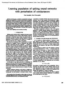
Fig. 1. Average test errors for class-switching ensembles composed of neural networks (solid lines in the plot) and decision trees (trait lines in the plot) using pˆ = 2/5 (bottom curves) and pˆ = 4/5 (top curves) for the Waveform dataset
Figure 1 displays the evolution with the number of base classifiers of the average generalization error (over 10 executions) for class-switching ensembles composed of neural networks (shown with solid lines in the plot) and decision trees (with trait lines) for the Waveform dataset. The number of hidden units for the networks is 28, and 1000 epochs were used for the training process. The bottom curves correspond to a pˆ value of 2/5 and the top curves correspond to pˆ = 4/5. The leaning curves displayed in this figure show that the generalization errors of the class-switching neural ensembles generated in this way are similar to those produced by decision trees class-switching ensembles. However, since the baseline performance given by a single decision tree is different from the performance of a neural net, the conclusions are different for ensembles composed of decision trees and for ensembles of neural networks. The improvement obtained by decision tree class-switching ensembles over a single tree is substantial (the generalization error of a single decision trees is ≈ 30%). Hence, for decision trees, the strategy of generating 0-error base learners seems to perform well. The piecewise-constant boundaries produced by single trees evolve to more complex and convoluted decisions boundaries when the decisions of the individual trees are combined in the ensemble. In contrast, the results obtained by the neural ensembles show that this strategy does not lead to ensembles that significantly improve the classification accuracy of a single network. In particular, a single neural network with 7 hidden units and trained with 500 epochs achieves an error rate of 19.3%, a
result that is equivalent to the final error of the neural class-switching ensemble of networks with zero error on the perturbed training set with pˆ = 4/5 (19.0%). In contrast, class-switching or bagging ensembles composed of 100 neural nets with only about 6 hidden units trained in the same conditions obtain a generalization error of ≈ 16.4%, which is a significant improvement over the configuration that uses more complex nets and larger ensembles. Note that a neural net with this number hidden units does not necessarily obtain a 0-error model on the modified training data. Nonetheless, this ensemble of simple networks is trained much faster and exhibits better generalization performance than an ensemble of complex networks trained to exhibit zero error on the perturbed versions of the training set.
3
Experiments
To assess the performance of the proposed method we carry out experiments in ten datasets from the UCI repository [23] and in two synthetic datasets (proposed by Breiman et al. [24, 5]). The datasets were selected to sample a variety of problems from different fields of application. The characteristics of the selected datasets, of the testing method and the networks generated are shown in Table 1. Table 1. Characteristics of the datasets, testing method, number of input units, average number (± standard deviation) of hidden units and average number of training epochs for the neural networks used in the experiments Dataset Breast W. Diabetes German Heart Labor New-thyroid Sonar Tic-tac-toe Twonorm Vehicle Waveform Wine
Instances
Test
699 768 1000 270 57 215 208 958 300 846 300 178
10-fold-cv 10-fold-cv 10-fold-cv 10-fold-cv 10-fold-cv 10-fold-cv 10-fold-cv 10-fold-cv 5000 cases 10-fold-cv 5000 cases 10-fold-cv
Attrib. Classes Input units 9 2 9 8 2 8 20 2 61 13 2 23 16 2 37 5 3 5 60 2 60 9 2 27 20 2 20 18 4 18 21 3 21 13 3 13
Hidden units 4.12±1.49 5.36±1.62 4.98±1.65 4.84±1.70 4.42±1.54 16.2±3.55 5.14±1.46 4.38±1.50 4.36±1.61 11.7±3.19 5.56±1.45 5.88±1.43
Training epochs 328 364 173 201 405 618 331 200 330 810 511 435
The base classifiers are feedforward neural networks with one hidden layer. We use sigmoidal transfer functions for both the hidden and output layers. The neurons are trained using an improved RPROP batch algorithm [25]. The optimal architecture and number of training epochs for the neural networks is estimated for every partition of the training data using cross validation. The same
architecture and number of epochs was used in bagging and class-switching ensembles. For the neural networks, the FANN library [26] implementation is used. The results given are averages of a 100 experiments for each dataset. In the real-world datasets these experiments consisted in the execution of 10 × 10fold-cv. For the synthetic datasets (Twonorm and Waveform) each experiment involves a random sampling to generate the training and testing sets (see Table 1 for the sizes of the sets). In general, each experiment involved the following steps: 1. Obtain the random training/testing datasets from the corresponding fold in the real-world datasets and by random sampling in the synthetic ones. 2. Build a single neural network using the whole training dataset. The configuration of the network is estimated using cross-validation of 10-fold in the training data. Different architectures (3, 5, and 7 hidden units) and different values for the number of epochs (100, 300, 500 and 1000) are explored. The configuration that obtains on average the best accuracy on the separate folds of the training data, is used. For some datasets the range of possible hidden units was incremented. For the Vehicle data set it was necessary to test 5, 7, 11, and 15 hidden units and for New-thyroid the tested architectures were 7, 11, 15 and 20. 3. Build the neural networks ensembles using class-switching (with pˆ values of: 0/5, 1/5, 2/5, 3/5 and 4/5) and bagging and using the configuration obtained for the single net. Note that class-switching with pˆ = 0/5 can not be considered a class switching algorithm: the variability in the ensemble is achieved solely by the training process converging to different weight values because of the different random initial values used. 4. Estimate the generalization error of the classifiers (single NN, bagging and class-switching) on the testing set. Figure 2 displays the average generalization error curves for bagging and class-switching ensembles for four datasets (German, Heart, Labor and Newthyroid). These plots show that the convergence of the error class-switching ensembles is related to the fraction of switched examples (i.e. pˆ): Higher pˆ values result in slower convergence. From these plots we observe that combining 200 networks is sufficient to reach convergence for most of the ensemble configurations. However, in some datasets (see German and Labor datasets in Fig. 2) with a high class-switching probability (class-switching with pˆ = 4/5), 200 is not sufficient to reach the asymptotic ensemble error rate. Table 2 presents the average test errors over the 100 executions for single networks, bagging and class-switching ensembles for the different values of pˆ. The lowest generalization error for every dataset is highlighted in bold-face. The standard deviations are given after the ± sign. These results show that class-switching ensembles exhibit the best results in nine of the twelve problems analyzed (2 × pˆ = 1/5, 2 × pˆ = 2/5, 5 × pˆ = 3/5 and 3 × pˆ = 4/5). Bagging has the best performance in two datasets and ensembles with pˆ = 0/5 also in two dataset. The performance of a single network is suboptimal in all cases investigated and is poorer than most of the different ensembles.
german 0.3 0.29
0.27
bagging p=0.0 p=0.1 p=0.2 p=0.3 p=0.4
0.28 0.26 0.24 error
0.28 error
heart 0.3
bagging p=0.0 p=0.1 p=0.2 p=0.3 p=0.4
0.22 0.2
0.26
0.18 0.25
0.16
0.24
0.14 0
20
40
60
80
100 120 140 160 180 200
0
20
40
number of classifiers
0.35
0.25
bagging p=0.0 p=0.1 p=0.2 p=0.3 p=0.4
0.13 0.12
error
error
0.3
100 120 140 160 180 200
new-thyroid 0.14
bagging p=0.0 p=0.1 p=0.2 p=0.3 p=0.4
0.4
80
number of classifiers
labor 0.45
60
0.11 0.1 0.09 0.08
0.2
0.07
0.15
0.06
0.1
0.05
0.05
0.04 0
20
40
60 80 100 120 140 160 180 200 number of classifiers
0
20
40
60 80 100 120 140 160 180 200 number of classifiers
Fig. 2. Average test errors for the German Credit (top left plot ), Heart (top right plot), Labor Negotiations (bottom left plot) and New-thyroid (bottom right plot) datasets
Table 2 shows that most configurations of class-switching ensembles reach similar generalization errors for most datasets. In particular, the same error rate is achieved in Waveform by class-switching with pˆ = 1/5, 2/5 and 3/5 and nearly the same results (within 0.2 points) are obtained in Diabetes, German, Tic-tactoe, Twonorm and Wine. The pˆ = 4/5 configuration exhibits significantly worse results in German, Labor, Sonar and Tic-tac-toe. In some cases this is due to the fact that larger ensembles ought to have been used. Table 3 shows the p-values of the paired t-test for the differences between bagging and class-switching ensembles using the different values of pˆ. Significant differences against class-switching have been underlined and statistically significant differences in favor of class-switching are high-lighted in bold-face. The last row of Table 3 displays the win/draw/loss records, where the first (second / third) numbers displayed in each cell correspond to the number of sets in which the algorithm displayed in the topmost row of the table wins (draws / losses) with respect to bagging. These records show that class-switching ensembles with pˆ = 1/5 and pˆ = 2/5 never perform worse than bagging and that they outperform bagging in some of the studied datasets. Class-switching with pˆ = 3/5 and pˆ = 4/5 outperforms bagging in several datasets but also performs significantly worse than bagging in other datasets.
Table 2. Average generalization errors Dataset
NN
Breast 3.9±2.5 Diabetes 25.9±4.7 German 26.2±5.4 Heart 17.0±7.9 Labor 8.6±12 New-thyroid 5.3±4.7 Sonar 23.5±8.8 Tic-tac-toe 2.2±1.8 Twonorm 3.8±0.7 Vehicle 19.4±4.0 Waveform 20.6±8.0 Wine 5.1±5.0
Bagging 3.9±2.4 24.9±4.6 24.7±5.9 21.1±13 8.4±12 5.8±5.1 20.2±8.7 1.8±1.3 3.1±0.4 17.0±4.1 16.4±1.0 2.2±3.7
0/5 3.8±2.4 24.8±4.7 25.0±6.2 16.4±7.8 7.2±11 5.0±4.6 21.3±8.4 1.9±1.4 3.5±0.6 15.9±3.6 16.4±1.0 2.0±3.4
Class-switching (ˆ p =) 1/5 2/5 3/5 3.8±2.4 3.7±2.2 3.3±2.3 24.9±4.5 24.8±4.2 24.8±4.4 24.8±5.9 24.9±5.9 24.7±6.0 16.0±7.6 16.2±7.4 16.3±7.3 6.6±11 7.5±12 10.8±15 4.6±4.2 4.2±4.0 4.2±3.9 21.0±8.5 21.1±9.2 21.6±9.3 1.8±1.3 1.8±1.2 1.7±1.2 3.1±0.4 2.9±0.4 2.9±0.5 16.1±3.5 16.4±3.7 17.1±3.7 16.5±1.0 16.5±0.9 16.5±1.0 1.6±2.8 1.4±2.7 1.5±3.0
4/5 3.3±2.3 24.6±4.7 25.7±6.4 16.6±7.4 14.5±16 4.4±3.8 23.2±9.6 7.7±5.5 3.3±1.1 17.8±3.3 16.6±0.9 1.2±2.6
Table 3. Results of a paired t-test for the differences between the test errors of bagging ensembles and class-switching ensembles Dataset 0/5 Breast 8.6·10−1 Diabetes 7.0·10−1 German 1.0·10−1 Heart 8.6·10−5 Labor 2.6·10−1 New-thyroid 2.5·10−2 Sonar 3.6·10−2 Tic-tac-toe 6.0·10−3 Twonorm 5.1·10−21 Vehicle 1.5·10−5 Waveform 4.6·10−1 Wine 4.8·10−1 3/6/3
4
class-switching (ˆ p =) 1/5 2/5 3/5 6.1·10−1 7.7·10−2 8.3·10−6 8.2·10−1 5.5·10−1 7.3·10−1 2.7·10−1 2.5·10−1 1.0·100 3.0·10−5 6.9·10−5 1.0·10−4 1.1·10−1 4.4·10−1 9.2·10−2 4.5·10−3 4.5·10−4 2.1·10−4 1.2·10−1 1.3·10−1 4.6·10−2 1.8·10−1 1.0·10−1 9.6·10−2 2.3·10−1 7.6·10−11 4.5·10−7 2.4·10−4 3.5·10−3 7.1·10−1 8.6·10−2 1.8·10−1 2.3·10−1 1.7·10−2 3.9·10−3 4.7·10−2 4/8/0 5/7/0 5/6/1
4/5 8·10−7 3.7·10−1 3.2·10−4 2.6·10−4 9.5·10−5 1.9·10−3 2.2·10−4 5.1·10−19 2.5·10−1 4.5·10−3 2.0·10−2 3.0·10−3 4/2/6
Conclusions
In the present article we have analyzed the performance of class-switching ensembles [22] using neural networks as base classifiers. The class-switching ensembles generate a diversity of classifiers using different perturbed versions of the training set. To generate each perturbed set, a fraction of examples is selected at random and their class labels are switched also at random to a different label. The prescription used for decision trees (generate individual classifiers that achieve 0-error in the perturbed training datasets) is not to be the appropriate
configuration for neural networks ensembles constructed with class-switching. Combining neural networks whose architecture is designed by standard architecture selection techniques (and therefore do not necessarily achieve 0 error in the perturbed training datasets) produces significantly better results than ensembles composed of more complex nets that do achieve 0 error in the perturbed datasets. As a consequence, the number of base learners needed for the convergence of the ensembles to its asymptotic error level is smaller that in class-switching ensembles composed of decision trees. Class-switching ensembles of neural networks built according to this prescription exhibit a classification accuracy that is better or equivalent to bagging on the tested datasets. Class-switching ensembles with pˆ = 1/5 and 2/5 never obtain results that are statistically worse than bagging in the studied datasets. Classswitching ensembles with pˆ = 3/5 and 4/5 obtain significantly better generalization error over bagging in the same number of datasets as class-switching with pˆ = 1/5 and 2/5 but also obtain generalization errors significantly worse than bagging for some of the investigated datasets.
References 1. Schapire, R.E., Freund, Y., Bartlett, P.L., Lee, W.S.: Boosting the margin: A new explanation for the effectiveness of voting methods. The Annals of Statistics 12(5) (1998) 1651–1686 2. Freund, Y., Schapire, R.E.: A decision-theoretic generalization of on-line learning and an application to boosting. In: Proc. 2nd European Conference on Computational Learning Theory. (1995) 23–37 3. Quinlan, J.R.: Bagging, boosting, and C4.5. In: Proc. 13th National Conference on Artificial Intelligence, Cambridge, MA (1996) 725–730 4. Breiman, L.: Bagging predictors. Machine Learning 24(2) (1996) 123–140 5. Breiman, L.: Arcing classifiers. The Annals of Statistics 26(3) (1998) 801–849 6. Opitz, D., Maclin, R.: Popular ensemble methods: An empirical study. Journal of Artificial Intelligence Research 11 (1999) 169–198 7. Bauer, E., Kohavi, R.: An empirical comparison of voting classification algorithms: Bagging, boosting, and variants. Machine Learning 36(1-2) (1999) 105–139 8. Dietterich, T.G.: An experimental comparison of three methods for constructing ensembles of decision trees: Bagging, boosting, and randomization. Machine Learning 40(2) (2000) 139–157 9. R¨ atsch, G., Onoda, T., M¨ uller, K.R.: Soft margins for AdaBoost. Machine Learning 42(3) (2001) 287–320 10. Breiman, L.: Random forests. Machine Learning 45(1) (2001) 5–32 11. Hansen, L.K., Salamon, P.: Neural network ensembles. IEEE Trans. Pattern Anal. Mach. Intell. 12(10) (1990) 993–1001 12. Wolpert, D.H.: Stacked generalization. Neural Networks 5(2) (1992) 241–259 13. Perrone, M.P., Cooper, L.N.: When networks disagree: Ensemble methods for hybrid neural networks. In Mammone, R.J., ed.: Neural Networks for Speech and Image Processing. Chapman-Hall (1993) 126–142 14. Sharkey, A.J.C.: Combining Artificial Neural Nets: Ensemble and Modular MultiNet Systems. Springer-Verlag, London (1999)
15. Cantador, I., Dorronsoro, J.R.: Balanced boosting with parallel perceptrons. In: IWANN. (2005) 208–216 16. Valentini, G., Dietterich, T.G.: Bias-variance analysis of support vector machines for the development of svm-based ensemble methods. Journal of Machine Learning Research 5 (2004) 725–775 17. Kong, E.B., Dietterich, T.G.: Error-correcting output coding corrects bias and variance. In: Proceedings of the Twelfth International Conference on Machine Learning. (1995) 313–321 18. Ho, T.K.: C4.5 decision forests. In: Proceedings of Fourteenth International Conference on Pattern Recognition. Volume 1. (1998) 545–549 19. Dietterich, T.G., Bakiri, G.: Solving multiclass learning problems via errorcorrecting output codes. Journal of Artificial Intelligence Research 2 (1995) 263– 286 20. F¨ urnkranz, J.: Round robin classification. Journal of Machine Learning Research 2 (2002) 721–747 21. Breiman, L.: Randomizing outputs to increase prediction accuracy. Machine Learning 40(3) (2000) 229–242 22. Mart´ınez-Mu˜ noz, G., Su´ arez, A.: Switching class labels to generate classification ensembles. Pattern Recognition 38(10) (2005) 1483–1494 23. Blake, C.L., Merz, C.J.: UCI repository of machine learning databases (1998) 24. Breiman, L., Friedman, J.H., Olshen, R.A., Stone, C.J.: Classification and Regression Trees. Chapman & Hall, New York (1984) 25. Igel, C., H¨ usken, M.: Improving the rprop learning algorithm. In: Proceedings of the Second International Symposium on Neural Computation, ICSC Academic Press (2000) 115–121 26. Nissen, S.: Implementation of a fast artificial neural network library (fann). Technical report, Department of Computer Science, University of Copenhagen (2003)