Uncalibrated Visual Servoing of Robots Using a Depth ... - CiteSeerX

804

IEEE TRANSACTIONS ON ROBOTICS, VOL. 22, NO. 4, AUGUST 2006

Uncalibrated Visual Servoing of Robots Using a Depth-Independent Interaction Matrix Yun-Hui Liu, Senior Member, IEEE, Hesheng Wang, Student Member, IEEE, Chengyou Wang, and Kin Kwan Lam

Abstract—This paper presents a new adaptive controller for image-based dynamic control of a robot manipulator using a fixed camera whose intrinsic and extrinsic parameters are not known. To map the visual signals onto the joints of the robot manipulator, this paper proposes a depth-independent interaction matrix, which differs from the traditional interaction matrix in that it does not depend on the depths of the feature points. Using the depth-independent interaction matrix makes the unknown camera parameters appear linearly in the closed-loop dynamics so that a new algorithm is developed to estimate their values on-line. This adaptive algorithm combines the Slotine–Li method with on-line minimization of the errors between the real and estimated projections of the feature points on the image plane. Based on the nonlinear robot dynamics, we prove asymptotic convergence of the image errors to zero by the Lyapunov theory. Experiments have been conducted to verify the performance of the proposed controller. The results demonstrated good convergence of the image errors. Index Terms—Adaptive control, robot manipulator, uncalibrated camera parameters, visual servoing.

[34]. Two basic schemes, namely position-based control [11], [36] and image-based control [10], [13]–[16], have been developed. A position-based approach needs to estimate the threedimensional (3-D) position and orientation of the robot using visual information, and an image-based approach employs directly the projection signals of feature points on the image plane without estimating the 3-D position and orientation. A combination of the two schemes is called hybrid visual servoing [25], [40]. While each scheme has its own advantages and drawbacks, image-based controllers are more robust to disturbances and measurement noises. Existing methods can also be classified into kinematics-based and dynamic methods according to whether the nonlinear dynamics is taken into account in controller design. In this paper, we address image-based dynamic control of a robot manipulator in 3-D motion using a fixed camera whose intrinsic and extrinsic parameters are not known. A. Kinematics-Based Uncalibrated Visual Servoing

I. INTRODUCTION ISUAL servoing is an approach to control motion of a robot manipulator using visual feedback signals from a vision system. This has been one of the most active topics in robotics since the early 1990s. There are two possible configurations to set up a vision system for visual servoing. First, the camera can be mounted at the end-effector of the robot manipulator, and such a setup is called eye-in-hand system [1], [7], [14], [16], [18], [25], [30]. Second, the camera can be fixed at the position near the manipulator [2], [4], [17], [22], [32],

V

Manuscript received June 9, 2005; revised December 16, 2005. This paper was recommended for publication by Associate Editor P. Rives and Editor L. Parker upon evaluation of the reviewers’ comments. This work was supported in part by the Hong Kong Research Grant Council under Grant CUHK4217/ 03E, in part by a Chinese University of Hong Kong (CUHK) direct grant, in part by the National Science Foundation of China under Projects 60334010 and 60475029, and in part by the National University of Defense Technology under the Changjiang Professorship Program of the Ministry of Education of China. This paper was presented in part at the IEEE International Conference on Robotics and Biomimetics, China, August 2004, and in part at the IEEE International Conference on Robotics and Automation, Spain, April 2005. Y. H. Liu is with the Department of Automation and Computer-Aided Engineering, Chinese University of Hong Kong, Shatin, NT, Hong Kong. He is also with the Joint Center for Intelligent Sensing and Systems, National University of Defense Technology, Changsha, Hunan, China (e-mail: [email protected]. hk). H. Wang and K. K. Lam are with the Department of Automation and Computer-Aided Engineering, Chinese University of Hong Kong, Shatin, NT, Hong Kong. C. Wang is with the Joint Center for Intelligent Sensing and Systems, National University of Defense Technology, Changsha, Hunan 410073, China. Digital Object Identifier 10.1109/TRO.2006.878788

Obtaining accurate camera parameters is crucial to performance of an image-based visual controller because the image Jacobian or interaction matrix, which depends nonlinearly on the parameters, is widely used to map the image errors onto the joint space of the manipulator. It is well known that camera calibration is tedious and costly. To avoid this, tremendous efforts have been made to on-line estimation of the image Jacobian. For the eye-in-hand setup, Yoshimi and Allen [38] proposed an estimator of the image Jacobian for a peg-in-hole alignment task. Hosoda and Asada [16] used the Broyden updating formula to estimate the image Jacobian. Ruf et al. [33] proposed an on-line calibration algorithm for position-based visual servoing. Papanikolopoulos et al. [30], [31] developed an algorithm for estimating on-line the relative distance of the target with respect to the camera. Recently, Malis [26] proposed a visual servo controller invariant to changes in the camera intrinsic parameters. For the fixed camera configuration, Jagersand et al. [19] proposed a similar method to that in [11], [16]. Piepmeier et al. [32] developed a dynamic quasi-Newton method. Using the least square method, Lu et al. [24] developed an algorithm for calculating on-line the exterior orientation. Chen et al. [8] proposed a homography based adaptive tracking controller by estimating the unknown depth and object parameters. A theoretical and thorough analysis has been conducted by Hespanha et al. [15], [41] on what can be done with uncalibrated stereo vision systems. B. Dynamic Visual Servoing However, the methods mentioned above are based on kinematics only and the nonlinear forces in robot dynamics are ne-

1552-3098/$20.00 © 2006 IEEE

LIU et al.: UNCALIBRATED VISUAL SERVOING OF ROBOTS USING A DEPTH-INDEPENDENT INTERACTION MATRIX

glected. Many works [4], [6], [9], [17], [21], [22] pointed out the importance of dynamic visual servoing because the nonlinear forces affect not only control errors but also the stability. To compensate for the nonlinear forces, Carelli et al. [5] proposed an adaptive controller for the eye-in-hand setup. For the fixed camera configuration, Zergeroglu et al. [39] used the backstepping technique to design a robust controller, which produces globally uniformly ultimately bounded errors for plane motion of the manipulator. The controller in [3] gives rise to asymptotic convergence of the position error when the desired trajectory is persistently exciting. However, the aforementioned controllers assume that the camera is well calibrated. Xiao et al. [37] developed a hybrid controller for tracing trajectory on a plane in an uncalibrated workspace with a fixed camera. Kelly [20] proposed an asymptotically stable controller for position control of a planar manipulator. The controller in [34] assumes that the intrinsic parameters are known. The adaptive controllers proposed by Hsu et al. [17], Astolfi et al. [2], and Bishop and Spong [4] also apply to planar manipulators only. Consequently, no dynamic controller with guaranteed stability has been developed to cope with the unknown camera parameters as well as 3-D motion of the robot manipulator. C. Contribution of This Paper This paper proposes a new adaptive controller to regulate a set of feature points on the image plane to desired positions using visual feedback from a fixed camera whose intrinsic and extrinsic parameters are not known. One of the major problems that obstruct the development of adaptive visual servoing is the fact that the image Jacobian or the interaction matrix cannot be linearly parameterized by the camera parameters. To solve this problem, we propose a depth-independent interaction matrix, which is obtained by eliminating the depth in the traditional interaction matrix. Using this depth-independent interaction matrix in controller design, it is possible to make the unknown camera parameters appear linearly in the closed-loop dynamics. As a result, we can use an adaptive algorithm, similar to that proposed by Slotine and Li [35], to estimate the unknown parameters on-line. However, since the objective is to regulate the system’s output (the projection), instead of the state, we cannot achieve the asymptotic convergence of the image errors simply using the Slotine–Li algorithm. To guarantee the convergence of the image errors, in the parameter adaptation we combine the Slotine–Li algorithm with an on-line gradient descending minimization algorithm of the errors between the real and estimated image coordinates of the feature points. The on-line minimization algorithm is to ensure full rank of the estimated projection matrix corresponding to the estimated camera parameters. To compensate for the nonlinear scaling term corresponding to the depth, a quadratic feedback of the image errors is introduced in the control law. This is one of the major differences of our controller from existing ones. The Lyapunov method is used to rigorously prove asymptotic convergence of the image errors based on the full nonlinear dynamics of the robot manipulator. In order to verify the performance, experiments have been conducted on a 3-degree-of-freedom (DOF)robotmanipulator.Theexperimentalresultsdemonstrated good convergence of the image errors.

805

Fig. 1. Fixed camera setup for visual servoing.

The contribution of this paper can be summarized as follows: First, a depth-independent interaction matrix is proposed for mapping the image errors onto the joint space. Second, a dynamic controller using the uncalibrated visual feedback from a fixed camera has been developed for 3-D motion control of a robot manipulator. Moreover, a new adaptive algorithm has been developed to estimate the unknown intrinsic and extrinsic parameters of the camera. Finally, the asymptotic convergence of the image errors to zero has been rigorously proved by the Lyapunov method based on the nonlinear dynamics, and the performance of the controller has been verified by experiments. II. CAMERA AND ROBOT MODELS This section describes the assumptions and the problem statement and reviews the kinematics of the visual servoing system. A. Problem Statement In this paper, we consider a fixed camera setup in which a vision system is placed near a robot manipulator to monitor its motion (Fig. 1). A number of feature points marked on the endeffector are being traced by the vision system. To clarify our problem, the following assumptions are made. 1) The intrinsic parameters of the camera are not calibrated. 2) The extrinsic parameters, i.e., the homogeneous transform matrix between the camera and the robot are not known. 3) The camera under consideration is a pin-hole camera with the perspective projection. Denote by the number of the feature points selected on the manipulator. The feature points are projected onto the image plane of the camera. The problem addressed is defined as follows: Problem 1: Given the desired positions of the feature points on the image plane, design a proper joint input for the robot manipulator under the aforementioned assumptions such that the feature points asymptotically approach to the desired positions. To simplify the discussion, we will first address the problem of controlling one feature point, and then in Section IV will extend the method to multiple feature points. B. Notations In this paper, a bold capital letter represents a matrix and a bold lower case letter expresses a vector. An italic letter represents a scalar quantity. A matrix, or vector, and or scalar accomimplies that its value varies with time. panied with a bracket

806

Furthermore, let and denote the zero matrix, respectively. and the


identity matrix

the camera frame. Denote by the product of the matrix the homogenous transformation matrix , i.e.,

and

C. Kinematics As shown in Fig. 1, we set up three coordinate frames, namely the robot base frame, the end-effector frame, and the camera frame, to represent motion of the manipulator and the kinematic relation between the vision system and the manipulator. Denote vector , where the joint angle of the manipulator by a is the number of DOFs. Represent the homogeneous coordinates of the feature point with respect to the robot base frame by a vector . From the forward kinematics of the robot manipulator

(5) denotes the th row vector of the rotation matrix, and are the coordinates of the translation vector . The is called perspective projection matrix and its dimenmatrix sion is 3 4. Note that this matrix depends on the intrinsic and extrinsic parameters, independent of the position of the feature point. The (3) can be rewritten as where

(1) is the Jacobian matrix of the robot manipulator. where Denote the coordinates of the feature point with respect to the . Then camera frame by

(6) The depth of the feature point is given by

(2) where is the 4 4 homogeneous transform matrix from the is a conrobot base frame to the camera frame. Note that stant and unknown matrix, representing the unknown extrinsic parameters:

where is the 3 3 rotation matrix and denotes the 3 1 translational vector. Let

express the homogenous coordinates of the projection of the feature point on the image plane. Under the perspective projection model

(7) denotes the third row vector of the perspective prowhere jection matrix . It is important to note the following properties of matrix [12]. has a rank Property 1: The perspective projection matrix of 3. When the parameters are not calibrated, the perspective projection matrix is unknown and thus should be estimated from coordinates of the feature points and their projections on the image plane. Note that there are 12 unknown components in the matrix. Since two equations correspond to one feature point, six feature points are necessary to estimate the perspective projection matrix. However, the following property should be noted. Property 2: Given the world coordinates of a sufficient number of feature points and their projections on the image can be determined plane, the perspective projection matrix only up to a scale. This can be easily explained by the fact that the matrix for any nonzero is a solution for (6) if is a solution because

(3) where is a 3 4 matrix determined by the intrinsic parameters of the camera

(4) where and are the scalar factors of the and axes of the image plane. represents the angle between the two axes. is the position of the principal point of the camera. in (3) is the depth of the feature point with respect to

From Property 2, the result is not unique no matter what estimator is employed. Therefore, we can fix one component of the unknown matrix , for example , so that 11 components need to be estimated. List the 11 unknown components in a vector denoted by , which is determined by the unknown camera intrinsic and extrinsic parameters, as follows:

where column.

denotes the component at the th row and the th


D. A Depth-Independent Interaction Matrix By differentiating (6), we obtain the following velocity relationship:

807

is a 3 1 vector whose third component is always Note that zero. From the perspective projection (6) and (7), we have

(14) (8) where the matrix form:

is a

Then, (13) can be rewritten as

matrix in the following (15) (9)

It should be noted that is the interaction by the matrix or image Jacobian, which differs from is independent on the depth of depth. Since the matrix the feature point, we call it depth-independent interaction maare linear to the comtrix. The components of matrix ponents of the perspective projection matrix . Proposition 1: The depth-independent interaction matrix has a rank of 2 if the rank of the perspective projection is 3. matrix is Proof: Assume that the rank of the matrix and smaller than 2. Then, there exist nonzero scalars such that (10) This equation can be written as (11) is not equal to zero, the If the coefficient are equation means that the three row vectors of the matrix linearly dependent. If the coefficient is zero, the first two row vectors are linearly dependent. However, the row vectors must has a rank of 3. be linearly independent because the matrix is 2. Consequently, the rank of the matrix Property 3: For any homogenous vector , the product can be written in the following linear form:

where , representing the estimation error. is a vector of the estimated parameters corresponding to the estiis indemated matrix . The 3 11 matrix estipendent of the unknown parameters. Here we call mated projection error of the feature point at time . can be calRemark 1: The estimated projection error culated from (13) without using the true camera parameters, though it can be represented explicitly as a linear function of , as shown in (15). of the unProposition 2: Suppose that an estimation known parameters leads to zero at five different positions of the feature point. If it is not possible corresponding to the to find that three of the five images positions are collinear, the estimated projection matrix has a rank of 3. The proof is given in Appendix. The conditions in Proposition 2 are illustrated in Fig. 15 in Appendix. Proposition 2 plays one of the most important roles in stability analysis of our controller. F. Robot Dynamics It is well-known that the dynamic equation of a robot manipulator has the form

is the where inertia matrix. that for any vector

(16) positive-definite and symmetric is a skew-symmetric matrix such

(12) is a regressor matrix without depending on the where intrinsic and extrinsic parameters of the camera and the vector represents the unknown camera parameters. E. An Estimated Projection Error of the Feature Point of the feature point and its correConsider a position at time instant . Denote an estimasponding projection by . We consider a tion of the unknown projection matrix fixed estimation at this moment and a time-varying one later in the adaptive rule. Define the following error vector:

(13)

The term represents the gravitational force, and is the joint input of the robot manipulator. The first term on the left side of (16) is the inertial force, and the second term represents the Coriolis and centrifugal forces. We will consider all the nonlinear dynamic forces in the controller design. III. ADAPTIVE IMAGE-BASED VISUAL SERVOING To cope with the unknown camera parameters, this section proposes a novel controller estimating the unknown parameters on-line while controlling motion of the manipulator. The adaptive control addressed here is different from traditional problems in robot control in which the state feedback errors are used. The errors to be fed back here are the image errors, i.e., pixels, which

808


are outputs of the system. In our problem, the state, e.g., the position and orientation of the robot manipulator, can also be obtained by the internal sensors, and thus the problem is slightly different from output adaptive control problems in nonlinear control theory. We propose to employ a hybrid scheme which feeds back both the position and velocity (state) of the manipulator and the image errors (output) as well. A. Controller Design Denote the desired position of the feature point on the image plane by , which is a constant vector. The image error is obtained by measuring the difference between the current position and the desired one:

Fig. 2. Selecting positions of the feature point on its trajectory for parameter adaptation.

From Property 3, the last term can be represented as a linear form of the estimation errors of the parameters as follows: (17) is the image error vector whose third component is always zero. Denote the time-varying estimation of the un. Using the estimated parameters, known parameters by we propose the following controller:

(20) where

, representing the estimation error and is a regressor matrix without depending on the unknown parameters. (18)

B. Estimation of the Camera Parameters

The first term is to cancel the gravitational force in the robot dynamics. The second term represents a velocity feedback in the joint space. The last two terms are the image error feedback. The matrix represents an estimation of the depth-indecalculated using the estimated pendent interaction matrix parameters. is an estimation of the third row vector of the is a positive-definite veperspective projection matrix. positive definite position gain locity gain matrix and is matrix. The rule for updating the estimation of the camera parameters will be described in next subsection. It should be noted that the controller does not use the inverse of the manipulator Jacobian or the depth-independent interaction matrix. does not It is important to note that the depth factor appear in control law. The quadratic form of in (18) is to compensate for the effect caused by the removal of the depth. Using the depth-independent interaction matrix and including the quadratic term are two important characteristics that differentiate our controller from other existing ones. It should be pointed out that the controller has a simple form suitable for real-time implementation. By substituting the control law (18) into the robot dynamics (16), we obtain the following closedloop dynamics:

In this subsection, we propose a new adaptive algorithm to estimate the unknown parameters on-line. The basic idea is to combine the Slotine–Li algorithm with an on-line minimization of the estimated projection error of the feature point in the gradient descending direction. Suppose that on its trajectory, at a time instant the feature and the corresponding projection point is at the position on the image plane is (Fig. 2). From (13) and (15), the estimated projection error of the feature point at this time instant is given by

(19)

(22)

(21) Even when is a constant, the error changes with time because the estimated parameters are time-varying. However, is a constant matrix once the regressor matrix the 3-D position of the feature point is fixed. It should be noted can be calculated from the measurement that the error of the 3-D position and projection of the feature point without knowing the true parameters, though the parameters appear in a linear form in (21). On the trajectory of the feature point, we can select such positions, and hence equations like (21) can be obtained. In the parameters adaptation, we update the estimation in the di. Folrection of reducing the estimated projection errors lowing is the adaptive rule for updating the estimation of the parameters:


where and are positive-definite and diagonal gain maand . trices, and their dimensions are, respectively, Note that the first term comes from the Slotine–Li algorithm and the second term represents on-line minimization of the estimated projection errors in the gradient descending direction. To simplify the notation, let (23) Remark 2: The adaptive algorithm is different from Slotine and Li’s algorithm because of the existence of the last term on the right side. The introduction of this term is to ensure fullrank of the estimated perspective projection matrix so that the asymptotic stability of the system is guaranteed. The selection of the positions is important for stability of the controller. The objective of introducing the last term in the adaptive rule is to ensure that the estimated projection matrix has a rank of 3. Proposition 2 states that five positions are sufficient and necessary to guarantee the full rank when the estimated projection errors are equal to zero and there are not three image projections lying on a line. Therefore, when selecting the five positions of the feature point, we must guarantee that any three of their projections on the image plane are not collinear. The following two methods can be used for the selection. • Method 1: Select the initial and current positions, and another three positions. The three positions can be obtained by arbitrarily moving the manipulator. This needs to be done off line when only one feature point is controlled. However, to control position of the end-effector of the robot, at least three non-collinear feature points must be selected, and hence the initial, goal, and current positions of the feature points can be used in the adaptive rule so that the off line process can be eliminated. constants • Method 2: Select . We can select the positions of the feature point on its trajectory at time with a condition that when . We can also select with a condition that the time-varying positions if . Since it is almost impossible for a manipulator to follow a straight line precisely, the conditions in Proposition 2 can be guaranteed if the number is reasonably large and the positions are randomly selected.

809

Proof: Introduce the following non-negative function:

(25) Multiplying the (19) results in

from the left to the closed-loop dynamics

(26) From (7) and (8), we have

(27) By multiplying the (22), we obtain

from the left to the adaptive rule

(28) Differentiating the function

in (25) results in

(29) From (1) and (7)

(30) By combining (26)–(30), we have

C. Stability Analysis We here analyze the stability of the robot manipulator under the control of the proposed controller and adaptive algorithm. For simplicity, we assume that the feature point is visible during the motion so that its depth with respect to the camera frame is always positive. Following is the main result of this paper. Theorem 1: If the five positions of the feature point for the parameter adaptation are so selected that it is impossible to find three collinear projections on the image plane, under the control of the proposed controller (18) and the adaptive algorithm (22) for parameters estimation, the image error of the feature point is convergent to zero, i.e.,

(31) never increases its value From this equation, the function so that it is upper bounded. From the definition (25), bounded directly implies that the joint velocity, the image errors, and the estimation errors are all bounded. Then, the joint accelerais bounded from the closed-loop dynamics (19) and tion from the adaptive algorithm (22). Therefore, the joint so is and the estimated parameters are uniformly velocity continuous. From the Barbalat Lemma, we conclude that

(24)

(32)

810


When and the points are so selected that the conditions in Proposition 2 are satisfied, the matrix has a rank of 3. To prove the convergence of the image error, we further consider the equilibrium points of the system. From the closed-loop dynamics (19) of the robot manipulator, at the equilibrium point, we have

denotes the depth of the feature point with where respect to the camera frame. The velocity relationship is given by

(37) has a similar form to the matrix in (9). From where the robot kinematics

(33) Note that the dimension of is three and its third compois a 4 3 nent is always zero. is a 3 3 matrix. matrix whose fourth row is due to the homogenous coordinates. is larger than or When the rank of the Jacobian matrix equal to three, at the equilibrium points, the following holds:

(38) is different It should be noted that the Jacobian matrix for different feature points. A controller similar to that in (18) can be designed by

(34) Note that (39)

(35) is three if the conditions The rank of the estimated matrix stated in Proposition 2 are satisfied. By using a similar proof to that for Proposition 1, it is possible to demonstrate that the has a rank of 2. From (34), it is obvious matrix that at the equilibrium point. Consequently, the image error is convergent to zero as the time approaches to the infinity. It should be pointed out that the estimated parameters are not convergent to the true values. If a sufficient number of positions of the feature point are selected for the adaptive algorithm, the convergence of the estimated projection errors implies that the parameters are convergent to the true values up to a scale. It should be also noted that the convergence of the image errors does not mean the convergence of the end-effector to the desired position. To regulate the end-effector in 3-D space, we need to properly select several feature points for control.

where (40) By substituting the control law (39) into the robot dynamics (16) and noting Property 3, we obtain the following closed-loop dynamics:

(41) The following adaptive rule, similar to that in (22), can be employed to estimate the unknown parameters:

IV. CONTROL OF MULTIPLE FEATURE POINTS In this section, we extend the proposed method to control of a number of feature points. Let be the number of the feature points. Denote the homogenous coordinates of feature point on the image plane by and its coordinates with respect to . Under the perspective projection the robot base frame by model, the coordinates are related by

(36)

(42) and denote, respectively, the th 3-D posiwhere tion of the feature point on its trajectory selected for parameter estimation and the corresponding projection on the image plane.


811

The number must be so selected that . The estiis similar to that in (21). mation error Theorem 2: Under the control of controller (39) and the adaptive rule (42), the position errors of the feature points are convergent to positions satisfying

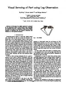
(43) Proof: Introduce the following non-negative function: Fig. 3. Experimental set-up.

(44) and from the left to the By multiplying the closed-loop dynamics (41), and the adaptive rule (42), respectively, we obtain

(45) A similar logic to that in the proof of Theorem 1 leads to that and are bounded, and hence that and are uniformly continuous. On the other hand, from the closed-loop dynamics (41) the equilibrium points must satisfy (43). Therefore, from Barbalat’s Lemma, the image errors are convergent to the equilibrium points satisfying (43) as the time approaches to the infinity. We further consider the convergence of the image error . It is not possible to conclude the convergence of the image errors to zero from (43) only. The image errors are convergent to zero only when the rank of the coefficient matrix

is equal to . This implies that the number of DOFs of the . When all the manipulator must be larger than or equal to feature points are on the end-effector and the end-effector is a rigid body, a stronger result can be obtained. Denote the position and orientation of the end-effector with respect to the robot base . The hoframe by a homogeneous transformation matrix mogenous coordinates of the feature point is given by (46) denotes the position of the feature point with respect where is a constant vector. to the end-effector frame. Note that Then, the image coordinates can be related as follows:

(47)

Once the image errors are convergent to the equilibrium points satisfying (43), the joint position and parameters estimates can be considered as constant vectors. We consider solution of for (43) provided that and are constants. Note that the can be represented by homogenous transformation matrix six independent unknowns, i.e., three translational and three rotational variables. By substituting (47) into (43), (43) represents nonlinear equations with six unknowns. When and the nonlinear equations admit a unique solution of the position and orientation of the end-effector, only one set of image coordisatisfies (43). Since nates for all is obviously a solution of (43), we can conclude the convergence of the image errors of the feature points to zero. If the nonlinear equations admit more than one solution, the image errors may not be convergent to zero. The conditions need to be further investigated in our future work. V. EXPERIMENTS We have implemented the proposed controller in a 3-DOF robot manipulator (Fig. 3) at the Networked Sensors and Robotics Laboratory of The Chinese University of Hong Kong. Experiments have been carried out to verify the performance of the proposed controller. The moment inertia about its vertical axis of the first link of the manipulator is 0.005 kgm , and the masses of the second and third links are 0.167 and 0.1 kg, respectively. The lengths of the second and third links are 0.145 and 0.1285 m, respectively. The joints of the manipulator are driven by Maxon brushed DC motors. The powers of the motors are 20, 10, and 10 W, respectively. The gear ratios at the three joints are 480:49, 12:1, and 384:49, respectively. Since the gear ratios are relatively small and the input motor powers are very small, the nonlinear forces have strong effect on the robot motion, though the manipulator is very light. We use three incremental optical encoders with a resolution of 2000 pulses/turn to measure the rotational angles of the motors. The joint velocities are obtained by differentiating the joint angles. A Ptgrey camera connecting with an Intel Pentium IV PC is used to capture image at the rate of 120 fps. The computer processes the image captured by the frame grabber and extracts the image features. The sampling period adopted in the experiments is 13 ms.

812


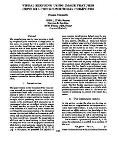
Fig. 4. Initial and desired (squared) positions of the feature point.

Fig. 6. Profile of the estimated parameters.

Fig. 5. Experiment result for one feature point when its five positions were used in the adaptive rule. (a) Position errors on the image plane. (b) Trajectory of the feature point on the image plane.

A. Control of One Feature Point In the first experiment, we control only one feature point marked on the end-effector. The coordinates of the feature point m. with respect to the end-effector frame are We first set the desired position of the feature point and record its image coordinates. Then move the end-effector to another

position and record that image coordinates as the initial position. Fig. 4 shows the initial and desired positions of the feature point on the image plane. Two experiments were conducted. In the first experiment, five positions of the feature point on its trajectory were selected for parameter adaptation. Fig. 5(a) and (b) demonstrate the position errors and the trajectory of the feature point on the image plane, respectively. The image error was within 1 pixel. The results confirmed the convergence of the image error to zero under control of the proposed method. Fig. 6 plots the profiles of the estimated parameters, which are not convergent to the true values. The fast convergence of the estimated parameters was due to the fast convergence of the image errors. Fig. 7 illustrates the 3-D trajectory of the end-effector. The initial and final and joint values of the manipulator are rad, respectively. It should be pointed out that the final position could be different for different running because one feature point cannot completely constrain the position of the end-effector. In the second experiment, we only used the current position of the feature point to construct the last term in the adaptive rule (22). Fig. 8 shows the image errors and the trajectory of the feature point on the image plane. Fig. 9 demonstrates the profiles of the estimated parameters. The results demonstrated that even when we only use the current position for parameters adaptation, it is still possible to achieve the convergence. This is because the last term, i.e., the estimated projection error, in the adaptive rule (22) is convergent very fast (Fig. 10). This experiment showed that it is possible to achieve the convergence without pre-selecting the observed positions, just by using the current position for the parameter estimation in the adaptive rule.


813

Fig. 7. 3-D trajectory of the end-effector.

Fig. 9. Estimated parameters.

Fig. 10. Profile of the estimated projection errors e(t).

The initial estimation of the homogenous transformation matrix of the robot base frame respect to the vision frame is

Fig. 8. Experimental result for one feature when only its current position is used in the adaptive rule. (a) Position errors on the image feature. (b) Trajectory of the feature point on the image plane.

The true intrinsic parameters and their initial estimations used in the experiment are given in Table I. The control gains used and . The adapwere and tive gains were

The true value of the homogenous transform matrix is not available. B. Control of Multiple Feature Points In the third experiment, we control three feature points whose coordinates with respect to the end-effector frames are

814


TABLE I CAMERA INTRINSIC PARAMETERS

Fig. 11. Initial and desired (squared) positions of the feature points.

, , and m, respectively. The initial and desired positions of the feature points are shown in Fig. 11. The trajectories and the image errors of the feature points on the image plane are demonstrated in Fig. 12. Fig. 13 plots the 3-D trajectory of the end-effector. Fig. 14 shows the profiles of the estimated parameters. The initial and final joint positions of the manipulator are, respectively, and rad. The experimental results confirmed that the image errors of the feature points are convergent to zero. The residual image errors are within one pixel. In this experiment, we employed three current positions of the feature points in the adaptive rule. The and control gains used the experiments are . The adaptive gains and are the same as those used in the previous experiments. The true values and initial estimations of the camera intrinsic parameters are as the same as those in Table I. The true camera extrinsic parameters were not available.

Fig. 12. Experimental results for three feature points. (a) Trajectories of the feature points on the image plane. (b) Image errors.

VI. CONCLUSION In this paper, we proposed an adaptive dynamic controller for position control of a number of feature points of a robot manipulator using uncalibrated visual feedback from a fixed camera. The controller employs a depth-independent interaction matrix, newly proposed, to map the image errors onto the joint space of the manipulator. By using the depth-independent interaction matrix, it is possible to make the unknown camera parameters appear linearly in the closed-loop dynamics of the system. A new adaptive algorithm has been developed to estimate the unknown intrinsic and extrinsic parameters. By taking the nonlinear dynamic forces of the robot into account, we proved, using the Lyapunov method, the asymptotic convergence of the image errors on the image plane to zero. Experiments have been carried out to verify the performance of the proposed method.

Fig. 13. 3-D trajectory of the end-effector.


815

Fig. 15. (a) Three projections of the feature point are on a line. (b) There are not three collinear projections on the image plane.

Proof: The statement at 2) is obvious, so no proof is given here. We only prove part 1). By submitting (48) into the perspective projection (6), we obtain (51) This equation can be rewritten as (52) Fig. 14. Estimated parameters.

To admit non-zero solution coordinates must satisfy

It should be noted that the discussion is focused on the fixed camera configuration. Extension of this method to an eye-inhand setup is our future work.

APPENDIX Here we prove Proposition 2 in detail. First, consider the following proposition. of Proposition 3: Suppose that the rank of an estimation the perspective projection matrix is not full so that its row vectors are related by

for (52), the image

(53)

We are now ready to prove Proposition 2. To guarantee that the estimated projection matrix has a rank of 3, we must ensure that there are at least three independent equations like (53) to and . constrain the coefficients Assume that five positions of the feature point lead to zero estimated projection errors. If three of the five projections are collinear on the image plane [Fig. 15(a)], Proposition 3 states that the three positions of the feature point may simultaneously yield

(48) and are not equal to zero. Assume where the coefficients that the projection of the feature point at the position yields the zero estimated projection error , i.e.,

(49) or 1) If efficients must satisfy

is not equal to zero, then the co-

(54) As a result, there are only two equations like (53) constraining the coefficients and , and hence feasible solutions exist. In other words, the rank of the estimated projection matrix is smaller than 3. On the other hand, if there are not three collinear projections on the image plane [Fig. 15(b)], there are at least three independent equations like (53) constraining the coefficients, and hence no feasible solution exists. Therefore, to guarantee that the rank of the estimated projection matrix is 3, the conditions stated in Proposition 2 must be satisfied.

(50) , the position vector must be on the 2) If intersection line between two planes defined by and in the 3-D space.

ACKNOWLEDGMENT The authors would like to thank the anonymous reviewers for their comments on the rigor of the proof of Theorem 1.

816


REFERENCES [1] P. K. Allen, A. Timcenko, B. Yoshimi, and P. Michelman, “Automated tracking and grasping of a moving object with a robotic hand-eye system,” IEEE Trans. Robot. Autom., vol. 9, no. 2, pp. 152–165, Apr. 1993. [2] A. Astolfi, L. Hsu, M. Netto, and R. Ortega, “Two solutions to the adaptive visual servoing problem,” IEEE Trans. Robot. Autom., vol. 18, no. 3, pp. 387–392, Jun. 2002. [3] B. Bishop, S. Hutchinson, and M. Spong, “Camera modeling for visual servo control applications,” Math. Comput. Model., vol. 24, no. 5/6, pp. 79–102, 1996. [4] B. Bishop and M. W. Spong, “Adaptive calibration and control of 2D monocular visual servo system,” in Proc. IFAC Symp. Robot Control, 1997, pp. 525–530. [5] R. Carelli, O. Nasisi, and B. Kuchen, “Adaptive robot control with visual feedback,” in Proc. Amer. Control Conf., 1994, pp. 1757–1760. [6] C. C. Cheah, M. Hirano, S. Kawamura, and S. Arimoto, “Approximate Jacobian control for robots with uncertain kinematics and dynamics,” IEEE Trans. Robot. Autom., vol. 19, no. 4, pp. 692–702, Aug. 2003. [7] F. Chaumette, “Potential problems of stability and convergence in image based and position based visual servoing,” in Confluence of Vision and Control. New York: Springer-Verlag, 1998, vol. 237, pp. 66–78. [8] J. Chen, D. M. Dawson, W. E. Dixon, and A. Behal, “Adaptive homography-based visual servo tracking,” in Proc. IEEE Int. Conf. Intell. Robots Syst., 2003, pp. 230–235. [9] L. Deng, F. Janabi-Sharifi, and W. J. Wilson, “Stability and robustness of visual servoing methods,” in Proc. IEEE Int. Conf. Robot. Autom., 2002, pp. 1604–1609. [10] B. Espiau, F. Chaumette, and P. Rives, “A new approach to visual servoing in robotics,” IEEE Trans. Robot. Autom., vol. 8, no. 3, pp. 313–326, Jun. 1992. [11] H. H. Fakhry and W. J. Wilson, “Modified resolved acceleration controller for position-based visual servoing,” Math. Comput. Model., vol. 24, no. 5/6, pp. 1–9, 1996. [12] D. A. Forsyth and J. Ponce, Computer Vision: A Modern Approach. Englewood Cliffs, NJ: Prentice-Hall, 2003. [13] E. Grosso, G. Metta, A. Oddera, and G. Sandini, “Robust visual servoing in 3-D reaching tasks,” IEEE Trans. Robot. Autom., vol. 12, no. 5, pp. 732–742, Oct. 1996. [14] K. Hashimoto, T. Kimoto, T. Ebine, and H. Kimura, “Manipulator control with image-based visual servo,” in Proc. IEEE Int. Conf. Robot. Autom., 1991, pp. 2267–2272. [15] J. Hespanha, Z. Dodds, G. D. Hager, and A. S. Morse, “What can be done with an uncalibrated stereo system,” in Proc. IEEE Int. Conf. Robot. Autom., 1998, pp. 1366–1372. [16] K. Hosada and M. Asada, “Versatile visual servoing without knowledge of true Jacobian,” in Proc. IEEE/RSJ Int. Conf. Intell. Robots Syst., 1994, pp. 186–191. [17] L. Hsu and P. L. S. Aquino, “Adaptive visual tracking with uncertain manipulator dynamics and uncalibrated camera,” in Proc. 38th IEEE Int. Conf. Decision Control, 1999, pp. 1248–1253. [18] S. Hutchinson, G. D. Hager, and P. I. Corke, “A tutorial on visual servo control,” IEEE Trans. Robot. Autom., vol. 12, no. 5, pp. 651–670, Oct. 1996. [19] M. Jagersand, O. Fuentes, and R. Nelson, “Experimental evaluation of uncalibrated visual servoing for precision manipulation,” in Proc. Int. Conf. Robot. Autom., 1997, pp. 2874–2880. [20] R. Kelly, “Robust asymptotically stable visual servoing of planar manipulator,” IEEE Trans. Robot. Autom., vol. 12, no. 5, pp. 759–766, Oct. 1996. [21] R. Kelly, F. Reyes, J. Moreno, and S. Hutchinson, “A two-loops direct visual control of direct-drive planar robots with moving target,” in Proc. IEEE Int. Conf. Robot. Autom., 1999, pp. 599–604. [22] D. Kim, A. A. Rizzi, G. D. Hager, and D. E. Koditschek, “A “robust” convergent visual servoing system,” in Proc. IEEE/RSJ Int. Conf. Intell. Robots Syst., 1995, pp. 348–353. [23] Y. H. Liu, K. Kitagaki, T. Ogasawara, and S. Arimoto, “Model-based adaptive hybrid control for manipulators under multiple geometric constraints,” IEEE Trans. Control Syst. Technol., vol. 7, no. 1, pp. 97–109, Jan. 1999. [24] C.-P. Lu, E. Mjolsness, and G. D. Hager, “Online computation of exterior orientation with application to hand-eye calibration,” Math. Comput. Model., vol. 24, no. 5/6, pp. 121–143, 1996.

[25] E. Malis, F. Chaumette, and S. Boudet, “Positioning a coarse-calibrated camera with respect to an unknown object by 2D 1/2 visual servoing,” in Proc. IEEE Int. Conf. Robot. Autom., 1998, pp. 1352–1359. [26] E. Malis, “Visual servoing invariant to changes in camera-intrisic parameters,” IEEE Trans. Robot. Autom., vol. 20, no. 1, pp. 72–81, Feb. 2004. [27] E. Malis and F. Chaumette, “Theoretical improvements instability analysis of a new class of model-free visual servoing methods,” IEEE Trans. Robot. Autom., vol. 18, no. 2, pp. 176–186, Apr. 2002. [28] P. Martinet and J. Gallice, “Position based visual servoing using a non-linear approach,” in Proc. IEEE/RSJ Int. Conf. Intell. Robots Syst., 1999, pp. 531–536. [29] A. Maruyama and M. Fujita, “Robust visual servo control for planar manipulators with the eye-in-hand configurations,” in Proc. 36th IEEE Conf. Decision Control, 1997, pp. 2551–2552. [30] N. P. Papanikolopoulos and P. K. Khosla, “Adaptive robotic visual tracking: Theory and experiments,” IEEE Trans. Autom. Control, vol. 38, no. 3, pp. 429–445, Mar. 1993. [31] N. P. Papanikolopoulos, B. J. Nelson, and P. K. Khosla, “Six degree-offreedom hand/eye visual tracking with uncertain parameters,” IEEE Trans. Robot. Autom., vol. 11, no. 5, pp. 725–732, Oct. 1995. [32] J. A. Piepmeier, G. V. McMurray, and H. Lipkin, “Uncalibrated dynamic visual servoing,” IEEE Trans. Robot. Autom., vol. 20, no. 1, pp. 143–147, Feb. 2004. [33] A. Ruf, M. Tonko, R. Horaud, and H.-H. Nagel, “Visual tracking of an end-effector by adaptive kinematic prediction,” in Proc. IEEE/RSJ Int. Conf. Intell. Robot. Syst., 1997, pp. 893–898. [34] Y. Shen, D. Song, Y. H. Liu, and K. Li, “Asymptotic trajectory tracking of manipulators using uncalibrated visual feedback,” IEEE/ASME Trans. Mechatron., vol. 8, no. 1, pp. 87–98, Mar. 2003. [35] J. J. Slotine and W. Li, “On the adaptive control of robot manipulators,” Int. J. Robot. Res., vol. 6, pp. 49–59, 1987. [36] W. J. Wilson, C. C. W. Hulls, and G. S. Bell, “Relative end-effector control using Cartesian position based visual servoing,” IEEE Trans. Robot. Autom., vol. 12, no. 5, pp. 684–696, Oct. 1996. [37] D. Xiao, B. Ghosh, N. Xi, and T. J. Tarn, “Intelligent robotic manipulation with hybrid position/force control in an uncalibrated workspace,” in Proc. IEEE Int. Conf. Robot. Autom., 1998, pp. 1671–1676. [38] B. H. Yoshimi and P. K. Allen, “Active, uncalibrated visual servoing,” in Proc. IEEE Int. Conf. Robot. Autom., 1994, pp. 156–161. [39] E. Zergeroglu, D. M. Dawson, M. S. de Queiroz, and S. Nagarkatti, “Robust visual-servo control of robot manipulators in the presence of uncertainty,” in Proc. 38th IEEE Int. Conf. Decision Control, 1999, pp. 4137–4142. [40] E. Malis, F. Chaumette, and S. Boudet, “2D 1/2 visual servoing,” IEEE Trans. Robot. Autom., vol. 15, no. 2, pp. 234–246, Apr. 1999. [41] J. P. Hespanha, Z. Dodds, G. D. Hager, and A. S. Morse, “What tasks can be performed with an uncalibrated stereo vision system?,” Int. J. Comput. Vis., vol. 35, no. 1, pp. 65–85, 1999.

Yun-Hui Liu (S’90–M’92–SM’98) received the B.Eng. degree in applied dynamics from Beijing Institute of Technology, Beijing, China, in 1985, the M.Eng. degree in mechanical engineering from Osaka University, Osaka, Japan, in 1989, and the Ph.D. degree in mathematical engineering and information physics from the University of Tokyo, Tokyo, Japan, in 1992. He wwas with the Electrotechnical Laboratory, MITI, Japan, from 1992 to 1995. Since February 1995, he has been with the Chinese University of Hong Kong, and is currently a Professor in the Department of Automation and Computer-Aided Engineering. He is also a ChangJiang Professor of the National University of Defense Technology and the Director of the Joint Center for Intelligent Sensing and Systems of the Chinese University of Hong Kong. He has published over 100 papers in refereed journals and refereed conference proceedings. His research interests include robot control multifingered robotic hands, mobile robots, virtual reality, Internet-based robotic systems, and machine intelligence. Dr. Liu received the 1994 and 1998 Best Paper Awards from the Robotics Society of Japan and the Best Conference Paper Awards (the first place in 2003 and the third place in 2000) of the IEEE Electro/Information Technology Conference. He was an Associate Editor of the IEEE TRANSACTIONS ON ROBOTICS AND AUTOMATION from 2001 to 2004. He is the General Chair of the 2006 IEEE/RSJ International Conference on Intelligent Robots and Systems (IROS).


Hesheng Wang (S’05) received the B.Eng. degree in electrical engineering from the Harbin Institute of Technology, Harbin, China, and the M.Phil. degree in automation and computer-aided engineering from the Chinese University of Hong Kong, Hong Kong, in 2002 and 2004, respectively. Currently, he is working toward the Ph.D. degree in the Department of Automation and Computer-Aided Engineering, Chinese University of Hong Kong. His research interests include visual servoing, adaptive robot control, and computer vision.

Chengyou Wang was born in Sichuan, China, on November 17, 1966. He received the B.Eng. degree in applied dynamics from the University of Information Engineering, China, in 1987, and the M.Eng. degree in communication engineering and the Ph.D. degree in signal processing from the National University of Defense Science and Technology, Hunan, China, in 1993 and 1997, respectively. He has been with the School of Electronic Science and Engineering, National University of Defense Science and Technology since 1997, and is now an As-

817

sociate Professor. He has published over 40 papers in refereed journals and conference proceedings. His research interests include speech processing, wireless communication, and active sensor network.

Kin Kwan Lam was born in Hong Kong in 1980. He received the B.Eng. degree in mechanical and automation engineering from the Chinese University of Hong Kong, Hong Kong, in 2002. Currently, he is working toward the M.Phil. degree in the Department of Automation and Computer-Aided Engineering, Chinese University of Hong Kong. His research interests include robot control and computer vision.