Combining UML and formal notations for modelling real-time systems Luigi Lavazza
Gabriele Quaroni
Matteo Venturelli
CEFRIEL - Politecnico di Milano P.za Leonardo da Vinci, 32 20133 Milano, Italia +39 02 23993553
Technology Reply srl Via Ripamonti, 89 20139 Milano, Italia +39 02 53576613
TXT e-solutions Via Frigia, 27 20126 Milano, Italia +39 02 257711
[email protected]
[email protected]
[email protected]
ABSTRACT This article explores a dual approach to real-time software development. Models are written in UML, as this is expected to be relatively easy and economic. Then models are automatically translated into a formal notation that supports the verification of properties such as safety, utility, liveness, etc. In this way, developers can exploit the advantages of formal notations while skipping the complex and expensive formal modelling phase. The proposed approach is applied to the Generalised Railroad Crossing (GRC) problem, one of the best known benchmarks proposed in the literature. A UML model of the GRC is built, and then translated into TRIO (a first order temporal logic). The resulting specification properties are tested by a history checking tool which exploits the formality of TRIO. The work described here highlights the shortcomings of UML as a real-time modelling language, proposes enhancements and workarounds to overcome UML limitations, and demonstrates the viability of using UML as a front-end for a formal real-time notation. By translating the GRC model into TRIO, we also give formal semantics to some of the UML constructs.
Keywords Real-time software, formal methods, UML.
1. INTRODUCTION Formal methods have been successfully employed in the development of several real-time software systems, where features like safety need to be formally proved. However, formal notations are generally considered too difficult or too expensive to be used in “ordinary” real-time software development, and it is a matter of fact that they are not widely employed. On the contrary, UML [5] is becoming extremely popular, essentially because it is a semiformal notation relatively easy to use (being mostly graphical),
and because it is provided with tools that support (although to a limited extent) code generation. However, UML was not conceived for modelling real-time software: its application in the real-time domain is limited by the lack of constructs to express time-related constraints and properties, as well as by the lack of formal semantics. This article explores a dual approach to real-time software development. In a first phase models are written in UML. This is expected to be a relatively economic activity, since UML does not require a big learning effort, and it is well supported by tools. In a second phase UML models are automatically translated into one or more formal notations, which provide support to activities such as the verification of properties (like liveness, safety, utility, …), test case generation, etc. In this way, developers exploit the advantages of formal notations while skipping the complex and expensive formal modelling phase. The optimal situation is when the derived models can be used by fully automatic tools: the modeller gets the results without even being aware of the underlying formal methods. As far as the formal notations are concerned, there are several possible candidates, such as the different extensions of the basic model of timed automata, e.g., linear hybrid systems, and timed automata with integer variables or multilabels. Actually, it can be useful to translate the same UML model into two or more notations, for instance into a declarative notation suited to support formal proofs, and into an operational one supporting simulation. The research activity from which this paper was derived is actually addressing the translation of UML models into TRIO, a first order theory augmented with a temporal domain that includes basic arithmetic [2] and Kronos timed automata, which come with a tool for model checking [8]. In this paper we cover only the usage of TRIO, because of space reasons, and because the integration with Kronos still needs some work. The proposed approach is applied to the Generalised Railroad Crossing (GRC) problem [3], one of the best known benchmarks proposed in the literature. The GRC was used both to understand the limitations of UML as a real-time modelling language, and as a test-bed for verifying the viability of the proposed approach: a UML model of the GRC was built, and then translated into TRIO.
results Model checker Model (notation1) UML CASE tool
UML models (XMI)
Test case generator
translators Model (notation2)
Simulator
Code generator
Figure 1. The envisaged environment. More precisely, the translation does not generally need to take into consideration the whole UML models: here we consider only state diagrams and –to some extent– class diagrams. The resulting specification properties were tested by a history checking tool which exploits the formality of TRIO. Of course it would be possible to exploit several other TRIO tools [7][11][12], but this was out of the scope of the research. In fact, the main goal of the research underlying the work presented here is to demonstrate the viability of a development process based on UML modelling and the translation of the resulting models into several different notations. The correctness and effectiveness of the formal methods that can then be used is given for granted.
and g(t)=90 indicating that the bar is up (gate open). A sequence of “occupancy intervals” is also defined, where each occupancy interval is a maximal time interval during which one or more trains are in I. Given two “positive tolerance” constants xi1 and xi2, the problem is to develop a system to operate the crossing gate that satisfies the following two properties:
-
Safety Property: The gate is closed during all occupancy intervals.
-
Utility Property: If t is not in any occupancy interval, nor within xi1 prior to an occupancy interval, nor within xi2 after an occupancy interval, then the gate is open.
The development environment that will originate from the work presented here (and which is currently being developed at CEFRIEL) is described in Figure 1.
I Gate
In order to validate the proposed approach, we applied it to the most critical part of a real-time system controlling a medical device. We do not report this experience here in detail for space reasons. The paper is organised as follows: Section 2 introduces the GRC problem, Section 3 illustrates the corresponding UML model – together with the extensions of the language– and properties. Section 4 deals with the translation of the UML model into TRIO. Section 5 discusses the proof of the model properties. Section 6 briefly accounts for related work, while in Section 7 some conclusions are drawn, and future work is sketched.
2. THE GRC PROBLEM 2.1 The definition The system to be developed operates a gate at a railroad crossing. The railroad crossing I lies in a region of interest R (see Figure 2). Trains travel through R on K tracks in both directions. Trains may proceed at different speeds, and can even pass each other. Only one train per track is allowed to be in R at any moment. Sensors indicate when each train enters and exits regions R and I. A gate function g from real times to the interval [0,90] describes the state of the gate, g(t)=0 indicating that the bar is down (gate closed)
R
Figure 2. The railroad crossing regions. Note that Figure 1 shows trains going in one direction. We adopt this simplification, since it has been demonstrated that the solution of the problem simplified in this way can be trivially extended to the general case.
2.2 Towards the solution of the GRC problem We introduce relevant points in the interest region (see Figure 3):
-
point RI indicates the position of the entrance sensor;
-
RO indicates the position of the exit sensor;
-
II indicates the position of the sensor which detects trains entering region I.
RI-RO defines zone R and II-RO defines zone I.
represent the gate and the position of the trains in each track within the interest region, respectively;
-
I dm g
dm-g
RI
X
II
RO
R
Crossing represents both the crossing region, belonging to the problem domain, and the controller, belonging to the solution domain.
It can be noticed that the proposed model is oversimplified: for instance, dm, dM, etc. should be functions of train speed and region lengths. Nevertheless, we decided not to represent items like trains, tracks, sensors, etc., in order to keep the model as simple as possible, while focusing on the specification of the realtime behaviour of the system. It is easy to enhance the model in order to include all the omitted details, and in order to reflect more faithfully the structure of the real system.
Figure 3. Annotated GRC. Crossing
Temporal constants describe maximum and minimum times for crossing the various zones, as well as the gate opening and closing times:
-
dm: minimum time taken by a train to cross RI-II zone; dM: maximum time taken by a train to cross RI-II zone;
-
hm: minimum time taken by a train to cross zone I (i.e., IIRO zone);
-
hM: maximum time taken by a train to cross zone I (i.e., IIRO zone);
-
g is the time taken by the bars of the gate for moving from the completely open to completely closed position (or vice versa).
Point X is thus defined as follows: when a train enters zone X-II it is time to start closing the gate, so that bars will be completely lowered when the train arrives at II (i.e., when the train enters the crossing zone I, or II-RO). We name RI-X and X-RO zones “Safe zone” and “Critical zone”, respectively. The exact position of X depends on the speed of each train, which is not known precisely. Thus the system cannot determine the right moment when a given train is at point X. However, it is clear that if we make the system safe for the fastest train, it will be safe also for the other trains. In order to have the gate closed when the fastest trains arrive at II, we must begin to close the gate dm-g seconds after the train entered region R. In this way when the fastest trains arrive at II the bars will be down and the crossing will be safe. Of course, the system will be safe for the slower trains as well. In order to assure the safety property, the bars must be raised only when the critical zone is empty. Conversely, in order to assure the utility property, the system must start opening the gate as soon as the critical zone becomes empty.
3. MODELLING THE GRC WITH UML 3.1 The class diagram We start modelling the GRC by defining the static structure of the model, by means of a class diagram (Figure 4). The following classes are defined:
-
Gate g : int
-
Gate and Train position, belonging to the problem domain,
CCR : int = 0 CIR : int = 0 dm : int dM : int 1
1
hm : int hM : int
close() : void open() : void
IncCCR() : void DecCCR() : void IncCIR() : void DecCIR() : void leaving() : void arriving() : void II(): void 1 K Train position
Figure 4. The class diagram of the GRC model. The Gate class is characterised by the constant opening and closing time g. The Gate class provides two methods, open and close, for opening and closing the gate, respectively. The Train position class represents the position of trains in each track of the interest region R. We are not interested in the exact position of trains, therefore the position is defined in an abstract way: out of region R, in RI-X, in X-II, in II-RO (see also Figure 5). The position of the train is determined according to the information provided by sensors, and taking into account the flowing of time. Whenever a train position changes (i.e., a train leaves a region and enters another one) this event is communicated to the controller, which reacts by sending appropriate commands to the gate. According to the specifications, there will be exactly K instances of this class, representing the trains travelling on the K tracks of R. Such a constraint is represented by specifying the number of instances involved in the relation linking the Crossing objects to the Train position objects. The Crossing class has only one instance, which represents the current situation and the criteria to be followed in sending
commands to the gate. The controller must always know how many trains are in the interest region, and how they are distributed into the different zones. To achieve this purpose we introduced the attributes CCR and CIR, which count how many trains are in the critical region and in zone I, respectively. Both counters are initially set to zero, and are modified by increment and decrement methods. Invariants concerning counters can be expressed by means of Object Constraint Language (OCL) [5] expressions: context Crossing inv : self.CCR>=0 context Crossing::IncCCR() inv : CCR@pre0 and CCR = CCR@pre-1 context Crossing inv : self.CIR>=0 and self.CIR= Self.dm Self.dm > Gate.g Self.hM >= Self.hm Self.hm > 0
3.2 State diagrams The state diagram of Train position class is reported in Figure 5. Initially the train is out of the interest region. When the sensor placed at RI sends its signal, the train is entering the safe zone. After dm-g seconds the fastest trains are at point X (i.e., entering the critical zone), thus we assume that the train is entering the Critical_zone, and the Crossing object is notified by means of an Arriving event. This transition is governed by a time-out, modelled by means of the After statement provided by UML [5]. Now we should specify that the train enters region I not earlier than g seconds nor later than dM-(dm-g) seconds after entering the critical zone. UML does not provide any means to specify that a transition cannot happen before a given time. Similarly, UML does not allow to say that a transition (or the corresponding event) must occur before a given time. In order to express such constraints we had to introduce the Close_to_Crossing state and the Error state. Note that these states were introduced only because of the limits of UML. If we modelled the GRC directly in TRIO [4] we would not need such “artificial” states, which make the model unnecessarily complex. Note also that the Error state here just indicates that the behaviour of the system deviated from the specifications. In designing a real system, we would wish to substitute the Error state with some exception handling state, for the sake of robustness.
Out_of_zone RI Safe_zone After( dm-g ) ^Crossing.Arriving After( g )[ II ] Critical_zone After( g )[ not II ] After( dM-dm )[ not II ]
Close_to_Crossing II
Error
Crossing
After( hm )[ RO ] ^Crossing.Leaving After( hm )[ not RO ] Ready_to_exit After( hM-hm )[ not RO ]
RO ^Crossing.Leaving
Figure 5. State diagram of class Train position. Another problem is to specify what happens if a train reaches point II exactly after it has been in the Critical zone for g seconds (which actually happens, for the fastest trains). In such a case the train goes directly into the Crossing state, without passing for the Close_to_Crossing state. In order to express this constraint we borrowed UML conditions syntax, forcing their semantics to express the check of the occurrence of an event at a given moment (in plain UML conditions cannot contain references to events). The meaning we assign to this usage of the UML notation can be easily defined formally. For instance, the transition from Critical_zone to Close_to_Crossing in Figure 5 has the following meaning, expressed in temporal logic: ∀t ((∃ δ (∀t2 (t-δ1 ] / DecCCR; DecCIR
Out_of_I Zone_I_free
Figure 9. The modified state diagram of class Crossing
4. Translating the UML model into TRIO 4.1 Translation procedure The translation was defined by identifying fragments of state diagrams, and defining the corresponding TRIO axioms. For space reasons, we do not report here all the fragment types mentioned above, instead we introduce just the more representative, especially those dealing with real-time features and constraints. The definition of TRIO is reported in [2]. In order to make the paper as self-contained as possible, a brief introduction to the most common constructs of the language is reported in the appendix.
4.1.1 Initial and final states and state persistence The initial state of a class is characterised by the following TRIO axiom: Som(Initial_state ∧ AlwP(Initial_state))
which states that at some time the object is in state Initial_state, and previously the object was always in that state. Note that in the GRC system all the objects have the same lifetime as the whole system. This fact allows us to say that an object was in a given state always before some time. In other systems, where objects are created and destroyed during the system lifetime, we should
introduce a “Not_existent” state, indicating that the corresponding object does not exist (i.e., it has not yet been instantiated). Similarly, final states are characterised by an axiom that indicates that when the final state is reached, it will be never left: Becomes(Final_state) → AlwF(Final_state)
States are persistent, i.e., an object remains in the same state until some relevant event occurs. For instance, the permanence of an instance of Train position (Figure 5) in state Out_of_zone is represented by the following axiom: Becomes(Out_of_zone) → Untilie(Out_of_zone,RI)
which states that once the object enters state Out_of_zone (at time some t) it will remain in that state until event RI occurs (at some time t’>t). The meaning of the “ie” subscript notation is explained in the appendix.
4.1.2 Time-out transitions and event generation An example of time-dependent transition is given by the transition from Safe_zone to Critical_zone in the state diagram of class Train position (Figure 5). It is represented by the following axioms: Becomes(Safe_Zone) → Lastsie(Safe_Zone,dm-g) Lastedie(Safe_Zone,dm-g) → Becomes(Critical_zone) ∧ Arriving
The first axiom says that the train will remain in the Safe_Zone state for dm-g seconds, while the second axiom states that after that period the train will enter the Critical_zone state, and at the same time the event Arriving is generated.
4.1.3 Time-out transitions guarded by events The behaviour of an object may depend not only on time-outs, but also on the concurrent occurrence of events. An example of this kind of transition is given by the transitions from Critical_zone to Close_to_Crossing and Crossing in state diagram of class Train position (Figure 5). These transitions are represented by the following axioms: Becomes(Critical_zone) → Lastsie(Critical_zone,g) Lastedie(Critical_zone,g) ∧ ¬ II → Becomes(Close_to_Crossing) Lastedie(Critical_zone,g) ∧ II → Becomes(Crossing)
These axioms state that a train remains in the critical zone for g seconds. After exactly g seconds, if event II occurs the train goes into the Crossing state, otherwise it goes into the Close_to_Crossing state.
4.1.4 Transitions dependent on other transitions’ times In some cases a transition occurs at a time which depends on other transitions’ occurrence time. An example is given by the transition from Inverted to Down in the state diagram of class Gate (Figure 6). This transition is represented by the following axioms, where LastTime(E, t) indicates that the most recent occurrence of E was at time t: Becomes(Inverted) ∧ LastTime(open,t1) ∧ LastTime(close,t2) → Lastsie(Inverted,t2-t1) Lastedie(Inverted, t2-t1) ∧ LastTime(open,t1) ∧ LastTime(close,t2) → Becomes(Down)
The former axiom states that the permanence of the gate in state “Inverted” is equal to the time passed between the last pair of “close” and “open” events, i.e., t2-t1. The latter axiom states that after such period the gate is closed (bar down). Note that we could have simplified these axioms, considering that the last occurrence of event close caused the state to become Inverted, i.e., t2 is always the current time in the axioms above. Note also that here we consider ReceiveTime and SendTime to be equal (i.e., the transmission time of events is negligible). Had the transmission time been relevant, we would have modelled it explicitly, e.g., introducing a connecting element between the sensor and the gate.
4.2 Automatic translation We developed a tool that automates the translation of UML models into TRIO axioms. The translator is written in Java, it takes in input the XMI [10] file generated by a UML CASE tool (we employed Rational Rose [13] and ARGO/UML [14]), parses it (by means of standard libraries provided by W3C) and applies the rules described above in order to generate TRIO axioms. Currently the user needs to edit the XMI file in order to make it compliant with the extensions of UML we defined, since these
extensions are not supported by available tools like Rose or Argo. This problem is dealt with in Section 7.
4.3 TRIO specifications Here we report the TRIO specification of the first model introduced in Section 3, i.e., the one concerning the single track case. Then we also discuss how to deal with the generalised case. The specifications reported here were obtained by means of the translator mentioned above.
4.3.1 Class Train position {Possible states and mutual exclusion} (Out_of_zone ∨ Safe_zone ∨ Critical_zone ∨ Close_to_Crossing ∨ Crossing ∨ Ready_to_Exit ∨ Error) Out_of_zone → ¬ (Safe_zone ∨ Critical_zone ∨ Close_to_Crossing ∨ Crossing ∨ Ready_to_Exit ∨ Error) Safe_zone → ¬ (Out_of_zone ∨ Critical_zone ∨ Close_to_Crossing ∨ Crossing ∨ Ready_to_Exit ∨ Error) Critical_zone → ¬ (Out_of_zone ∨ Safe_zone ∨ Close_to_Crossing ∨ Crossing ∨ Ready_to_Exit ∨ Error) {other formulae imposing mutual exclusion of states are omitted} {Transitions} Som(Out_of_zone ∧ AlwP(Out_of_zone)) UpToNow(Out_of_zone) ∧ RI → Becomes(Safe_Zone) Becomes(Safe_Zone)→ Lastsie(Safe_Zone,dm-g) Lastedie(Safe_Zone,dm-g) → Becomes(Critical_zone) ∧ Arriving Becomes(Critical_zone) → Lastsie(Critical_zone,g) Lastedie(Critical_zone,g) ∧ ¬ II → Becomes(Close_to_Crossing) Becomes(Close_to_Crossing) → Untilie(Close_to_Crossing, II ∨ Lastedie(Close_to_Crossing,dM-dm)) Lastedie(Critical_zone,g) ∧ II → Becomes(Crossing) Lastedie(Close_to_Crossing,dM-dm) ∧ ¬ II → Becomes(Error) Becomes(Error) → AlwF(Error) UpToNow(Close_to_Crossing) ∧ II → Becomes(Crossing) Becomes(Crossing) → Lastsie(Crossing,hm) Lastedie(Crossing,hm) ∧ RO → Becomes(Out_of_zone) ∧ Leaving Lastedie(Crossing,hm) ∧ ¬ RO → Becomes(Ready_To_Exit) Becomes(Ready_To_Exit)→ Untilie(Ready_To_Exit, RO ∨ Lastedie(Ready_To_Exit,hM-hm)) Lastedie(Ready_To_Exit,hM-hm) ∧ ¬ RO → Becomes(Error) UpToNow(Ready_To_Exit) ∧ RO → Becomes(Out_of_zone) ∧ Leaving Becomes(Out_of_zone) → Untilie(Out_of_zone,RI)
4.3.2 Class Gate {Possible states and mutual exclusion} (Up ∨ MvDown ∨ MvUp ∨ Down ∨ Inverted ) Up → ¬ (MvDown ∨ MvUp ∨ Down ∨ Inverted MvDown → ¬ (Up ∨ MvUp ∨ Down ∨ Inverted MvUp → ¬ (Up ∨ MvDown ∨ Down ∨ Inverted Down → ¬ (MvDown ∨ MvUp ∨ Up ∨ Inverted Inverted → ¬ (MvDown ∨ MvUp ∨ Down ∨ Up
) ) ) ) )
{Transitions} Som(Up ∧ AlwP(Up)) UpToNow(Up) ∧ Close → Becomes(MvDown) Becomes(MvDown) → Lastsie(MvDown,g) Lastedie(MvDown,g) → Becomes(Down) Becomes(Down) → Untilie(Down,Open) UpToNow(Down) ∧ Open → Becomes(MvUp) Becomes(MvUp) → Untilie(MvUp, Close ∨ Lastedie(MvUp,g)) UpToNow(MvUp) ∧ Close → Becomes(Inverted) Becomes(Inverted) → Lastsie(Inverted,t2-t1) ∧ LastTime(open,t1) ∧ LastTime(close,t2) Lastedie(MvUp,g) ∧ ¬ Close → Becomes(Up) Becomes(Up) → Untilie(Up,Close) Lastedie(Inverted, t2-t1) ∧ LastTime(open,t1) ∧ LastTime(close,t2) → Becomes(Down)
4.3.3 Class Crossing {Possible states and mutual exclusion} Empty_Opening ∨ Empty_Open ∨ Not_Empty Empty_Opening → ¬ Empty_Open ∧ ¬ Not_Empty Empty_Open → ¬ Empty_Opening ∧ ¬ Not_Empty Not_Empty → ¬ Empty_Open ∧ ¬ Empty_Opening {Substates of Not_Empty} Not_Empty ↔ Zone_I_occupied ∨ Zone_I_free Zone_I_occupied → ¬ Zone_I_free Zone_I_free → ¬ Zone_I_occupied {Operations} IncCCR ∧ CCR(X) → Becomes(CCR(X+1)) DecCCR ∧ CCR(X) → Becomes(CCR(X-1)) Becomes(CCR(X)) → Untilie(CCR(X),IncCCR ∨ DecCCR)
CCR(X) → ¬ CCR(Y) ∧ X ≠ Y {axioms for CIR, IncCIR and DecCIR are omitted, being similar to those concerning CCR, IncCCR and DecCCR} {Transitions} Som(Empty_Open ∧ AlwP(Empty_Open)) Empty_Open ∧ AlwP(Empty_Open) → CCR(0) ∧ CIR(0) UpToNow(Empty_Open) ∧ Arriving → Becomes(Zone_I_free) ∧ Close ∧ IncCCR UpToNow(Empty_Opening) ∧ Arriving → Becomes(Zone_I_free) ∧ Close ∧ IncCCR Not_Empty ∧ Arriving → IncCCR Becomes(Zone_I_free) → Untilie(Zone_I_free, II) UpToNow(Zone_I_free) ∧ II → Becomes(Zone_I_occupied) ∧ IncCIR Zone_I_occupied ∧ II → IncCIR Zone_I_occupied ∧ Leaving ∧ CCR(X) ∧ X>1 → DecCCR ∧ DecCIR Becomes(Zone_I_occupied) → Untilie(Zone_I_occupied, Leaving ∧ CIR(1)) UpToNow(Zone_I_occupied) ∧ Leaving ∧ CCR(1) ∧ CCR(1) → Becomes(Empty_Opening) ∧ DecCCR ∧ DecCIR ∧ Open UpToNow(Zone_I_occupied) ∧ Leaving ∧ CCR(X) ∧ X>1 → Becomes(Zone_I_free) ∧ DecCCR ∧ DecCIR Becomes(Empty_Opening) → Lastsie(Empty_Opening, g) Lastedie(Empty_Opening, g) → Becomes(Empty_Open) Becomes(Empty_Open) → Untilie(Empty_Open, Arriving)
4.3.4 Dealing with the generalised case The TRIO specifications for the generalized case are derived from the UML model of the generalized railroad crossing system (i.e.,
the model containing the state diagram given in Figure 8). With respect to the single track case, the translation has to take into account a few more issues, which are illustrated below. When there is just one track, at most one increment (or decrement) of CCR at a time is required. This situation is easily managed by means of sentences like the following: UpToNow(Empty_Open) ∧ Arriving → Becomes(Zone_I_free) ∧ Close ∧ IncCCR
When multiple tracks are considered, it is necessary to take into account what happens if multiple trains enter the critical zone at the same time. It is clear that the formula above would not work, since CCR would be incremented only once. In the general case (i.e., multiple tracks, each equipped with one sensor), several trains, travelling on different tracks, may activate at the same time the corresponding sensors. This case can be managed easily if we add the Track identifier as a parameter of event Arriving. This requires a trivial modification of the state diagram of class Train position reported in Figure 8: e.g., the transition from Safe_zone to Critical_zone should be labelled “After(dm-g)^Crossing.Arriving(Track)”. In fact, the parallel activation of several sensors can be easily recognised and dealt with by expressions like the following, which indicate that at any moment CCR must be incremented by the number of trains which are crossing point X and decremented of the number of trains which are crossing point RO at that moment:
∀j,v S(j,v) ↔ (S(j-1,v-1)∧Arriving(j) ∨ S(j-1,v+1)∧Leaving(j) ∨ S(j-1,v)∧
S(0,0) ∧
(¬Arriving(j) ∧ ¬Leaving(j))) CCR(X) ∧ S(K,Y) → Becomes(CCR(X+Y))
The first axioms assures that at any moment t S(K,Y) is true, where K is the number of tracks and Y is the number of Arriving events occurring at time t minus the number of Leaving events occurring at t. The second axiom states that the number of trains in the critical region (CCR(X)) is modified as indicated by S(K,Y). The same specification can be written in a non recursive way: Arriving(N) → DeltaC(N,1) Leaving(N) → DeltaC(N,-1) ¬Arriving(N) ∧ ¬Leaving(N) → DeltaC(N,0) CCR(X) ∧ DeltaC(1,X1) ∧ DeltaC(2,X2) ∧ … ∧ DeltaC(n,Xn)→ Becomes(CCR(X+X1+X2+…+Xn))
This is the only type of substantial modifications required to deal with the generalised case.
4.4 Dealing with non-determinism It is generally recognized that some amount of non-determinism can be useful in specifications. Our approach does not take into account non-determinism in the sense that for each of our state diagrams there is always only one transition which can occur, and thus only one active state. Nevertheless, we considered the possibility of modelling non-determinism in time, for instance to express that a given transition may occur at any moment within a given time interval. For instance, when modelling a sensor, we should say that signal II can follow signal RI after a time comprised between dm and
dM seconds. We represent this kind of constraints as illustrated by Figure 10.
Out After(t)[hm0 ∧ Past(F,δ) ∧ Lasted (F,δ)) {F held for a nonnull time interval that ended at the current instant} Becomes (F) def = F ∧ UpToNow(¬F) {F holds at the current instant but it did not hold for a nonnull interval that preceded the current instant} LastTime (F,t) def = Past(F,t) ∧ (Lastedei (¬F,t)) {F occurred for the last time t units ago}
Notice that the operators expressing a duration over a time interval (for example Lasts) are given definitions where the extremes of the specified time interval are excluded, i.e. the interval is open. Operators including either one or both of the extremes can be easily derived from the basic ones we listed above. For notational convenience, in order to indicate inclusion or exclusion of the lower or upper bound of the interval, we append to the operator name two subscripts, ‘i’ or ‘e’, respectively. For example, Lastsie and Lastsei are defined as follows.
Lastsie(A,t) def = Lastsei(A,t) def =
A ∧ Lasts(A,t) Lasts(A,t) ∧ Dist(A,t)
The former axiom states that A is true at the current instant and for an open interval of duration t. The latter statement states that A is true for an open interval of duration t and at a time instant whose distance is exactly t time units from the current instant.