IEEE TRANSACTIONS ON IMAGE PROCESSING, VOL. 21, NO. 3, MARCH 2012
1211
Completely Automated Multiresolution Edge Snapper—A New Technique for an Accurate Carotid Ultrasound IMT Measurement: Clinical Validation and Benchmarking on a Multi-Institutional Database Filippo Molinari, Member, IEEE, Constantinos S. Pattichis, Senior Member, IEEE, Guang Zeng, Luca Saba, U. Rajendra Acharya, Roberto Sanfilippo, Andrew Nicolaides, and Jasjit S. Suri, Senior Member, IEEE
Abstract—The aim of this paper is to describe a novel and completely automated technique for carotid artery (CA) recognition, far (distal) wall segmentation, and intima–media thickness (IMT) measurement, which is a strong clinical tool for risk assessment for cardiovascular diseases. The architecture of completely automated multiresolution edge snapper (CAMES) consists of the following two stages: 1) automated CA recognition based on a combination of scale–space and statistical classification in a multiresolution framework and 2) automated segmentation of lumen–intima (LI) and media–adventitia (MA) interfaces for the far (distal) wall and IMT measurement. Our database of 365 B-mode longitudinal carotid images is taken from four different institutions covering different ethnic backgrounds. The ground-truth (GT) database was the average manual segmentation from three clinical experts. The mean distance standard deviation of CAMES with respect to GT profiles for LI and MA interfaces were 0.081 0.099 and 0.082 0.197 mm, respectively. The IMT measurement error between CAMES and GT was 0.078 0.112 mm. CAMES was benchmarked against a previously developed automated technique based on an integrated approach using feature-based extraction and classifier (CALEX). Although CAMES underestimated the IMT value, it had shown a strong improvement in segmentation errors against CALEX for LI and MA interfaces by 8% and 42%, respectively. The overall IMT measurement bias for CAMES improved by 36% against CALEX. Finally, this paper demonstrated that the figure-of-merit of CAMES was 95.8% compared with 87.4% for CALEX. The combination of multiresolution CA recognition and far-wall segmentation led to an automated, low-complexity, real-time, and accurate technique for carotid IMT measurement. Validation on a multiethnic/multi-institutional Manuscript received January 29, 2011; revised August 11, 2011; accepted August 23, 2011. Date of publication September 22, 2011; date of current version February 17, 2012. The associate editor coordinating the review of this manuscript and approving it for publication was Prof. Margaret Cheney. F. Molinari is with the BioLab, Department of Electronics, Politecnico di Torino, 10129 Torino, Italy (e-mail:
[email protected]). C. S. Pattichis and A. Nicolaides are with the Department of Computer Science, University of Cyprus, 1678 Nicosia, Cyprus (e-mail:
[email protected]). G. Zeng is with the Mayo Clinic, Rochester, MN 55905 USA (e-mail:
[email protected]). L. Saba is with the Department of Radiology, Azienda Ospedaliero Universitaria, University of Cagliari, 09045 Cagliari, Italy. U. R. Acharya is with the Department of Electrical and Computer Engineering, Ngee Ann Polytechnic, Singapore 599489 (e-mail:
[email protected]). R. Sanfilippo is with the Department of Vascular and Thoracic Surgery, Azienda Ospedaliero Universitaria, University of Cagliari, 09042 Cagliari, Italy. J. S. Suri is with Global Biomedical Technologies, Inc., Roseville, CA 95661 USA, and also with the Biomedical Engineering Department, Idaho State University, Pocatello, ID 83209 USA (e-mail:
[email protected]). Digital Object Identifier 10.1109/TIP.2011.2169270
data set demonstrated the robustness of the technique, which can constitute a clinically valid IMT measurement for assistance in atherosclerosis disease management. Index Terms—Atherosclerosis, edge detection, first-order absolute moment, first-order Gaussian derivative, intima–media thickness (IMT), segmentation, ultrasound imaging.
I. INTRODUCTION
T
HE intima–media thickness (IMT) of the carotid artery (CA) is a widely accepted and validated marker of progression of atherosclerosis and of onset of cardiovascular disorders, with a predictive value for incident myocardial infarction [1]. IMT is usually measured by using ultrasound imaging. Normally, a trained sonographer manually measures the IMT from longitudinal projections of the CA, but these manual measurement methods are time consuming, subjective, and tedious. In addition, due to the lack of standardization, the differences in the gain settings, scanner performances, and the training of the clinicians all add up to cause significant variability, particularly in large and multicenter studies. Fig. 1 shows an example of a B-mode longitudinal carotid ultrasound image, with the far-wall IMT measurement depicted. Since the early 1990s, more than 30 different computer techniques have been developed for the segmentation of the CA wall in longitudinal images (a state-of-the-art review on the most used image processing techniques in carotid wall segmentation and IMT measurement can be found in a recent review by Molinari et al. [2]). Conceptually, there are two main groups of computer methods for IMT measurement: Group 1 comprises all the techniques that are completely automated, whereas group 2 comprises those that require user interaction (semiautomated). Usually, user-dependent methods offer better performance in IMT measurement, allowing measurement errors lower than 0.01 mm (an error in the range 1.25%–2.5%, since the normal value of IMT is about 0.4 mm at birth and 0.8 mm at 80 years if no vascular pathologies are present [3]). The most popular image processing techniques for CA wall segmentation and IMT measurement are based on image gradients and edge detection [4], [5] or parametric deformable models (so-called snakes) [6]–[8]. These detection techniques require
1057-7149/$26.00 © 2011 IEEE
1212
IEEE TRANSACTIONS ON IMAGE PROCESSING, VOL. 21, NO. 3, MARCH 2012
TABLE I CHARACTERISTICS OF THE IMAGE DATA SET COMING FOR FOUR DIFFERENT INSTITUTIONS AND RELATIVE PATIENT DEMOGRAPHICS. THE FIRST COLUMN REPORTS THE INSTITUTION, THE SECOND COLUMN SHOWS THE NUMBER OF IMAGES, THE THIRD COLUMN SHOWS THE CONVERSION FACTOR, THE FOURTH COLUMN SHOWS THE SCANNER USED, AND THE LAST TWO COLUMNS REPORT THE NUMBER OF PATIENTS AND THEIR DEMOGRAPHICS
Fig. 1. Reference anatomy of a longitudinal ultrasound image of a CA showing the LI interface, the MA interface, and the IMT.
user interaction for the region-of-interest (ROI) delineation around the distal (far) carotid wall. The aim of this paper is to develop a high-performance automated technique for carotid IMT measurement. We present a new strategy based on a two-cascaded-stage process. Stage-I combines an edge-detection approach based on a scale–space paradigm in a multiresolution framework, and Stage-II is the segmentation of lumen–intima (LI) and media–adventitia (MA) borders for the far wall using a combination of first-order absolute moment filtering followed by edge detection using a heuristic-based strategy. Stage-I comprises edge estimation for the far adventitia AD borders along the CA. This edge estimation uses derivatives of Gaussian kernels with known scales. The image processing paradigm comprises optimization of the right kernel size by reverse engineering the image framework itself. Stage-II comprises an edge detector based on the first absolute central moment (originally adapted by Faita et al. [4]) in the guidance zone (GZ) or ROI, followed by heuristic-based peak detection and location. We named our new technique completely automated multiresolution edge snapper (CAMES), as we used edge information in a multiresolution framework for both recognition and segmentation phases. Special precaution based on anatomic arterial information extracted using a statistical intensity distribution is embedded in Stage-I to ensure 100% accuracy during the automated recognition phase. We validated CAMES on a multiethnic multi-institutional database of 365 images, comprising normal and pathologic CAs. Finally, we benchmarked CAMES against CALEX, which is our previously developed automated technique [9], [10]. II. MATERIALS AND METHODS A. Image Data Set Our database consisted of 365 B-mode images collected from four different institutions. They are as follows: 1) the Neurology Division of the Gradenigo Hospital of Torino (Italy), which provided 200 images; 2) the Cyprus Institute of Neurology of Nicosia (Cyprus), which provided 100 images; 3) the Hospital de S. João do Porto (Portugal), which provided 23 images; and 4) the Department of Radiology of the University Hospital of Cagliari (Italy), which provided 42 images. The complete description of the image database and the patient’s demographics is reported in Table I. All the images were
acquired in digital format and discretized on 8 bits (256 gray levels). The conversion factors (i.e., the physical pixel dimension, which we indicate by in this paper) ranged from 0.06 to 0.09 mm/pixel. The conversion factors were different since they depended on the scanner type and scanner settings. The Institutions took care of obtaining written informed consent from the patients prior to acquiring data. The experimental protocol and data acquisition procedure were approved by the respective local Ethical Committees. For each of the 365 images, we had three manual segmentations made by expert sonographers [considered as ground truth (GT)]. To compute the IMT measurement bias, we obtained the average LI/MA tracings for every image. B. Architecture of CAMES The patented architecture under the class of AtheroEdge(R) systems called CAMES was developed by keeping in mind that it should be able to locate the CA in the image frame automatically and then segment the far wall of the CA by computing the two interface boundaries, namely, LI and MA interfaces. This recognition process must ensure that we are able to distinguish the CA layer from other arteries or veins, particularly the jugular vein (JV). We modeled the CA recognition process by taking the hypothesis that the CA’s far-wall adventitia is the brightest in the ultrasound scan frame. Our architecture for Stage-I is the recognition of the AD location in the gray-scale image of the CA using a multiresolution approach in a scale–space framework. Once the AD layer of the CA is recognized, Stage-II can be adapted for LI and MA border estimation in the gray-scale GZ near the AD layer. In summary, our architecture consists of the following two cascaded stages in a scale–space paradigm using a multiresolution framework adapting edge model approaches fused with heuristics: 1) automated recognition of the CA in the image frame and 2) automated segmentation of the far (distal) CA wall, i.e., the LI and MA border estimation process. Prior to recognition and segmentation phases, it is necessary to remove the nonrelevant information in the image, such as the patient and the device. We developed a simple automated cropping procedure that automatically cropped the image in order to discard the surrounding black frame containing device headers and image/patient text data [14].
MOLINARI et al.: CAMES—TECHNIQUE FOR ACCURATE CAROTID ULTRASOUND IMT MEASUREMENT
1213
Fig. 2. (a) Original cropped image. (b) Downsampled image. (c) Despeckled image. (d) Image after convolution with a first-order Gaussian derivative (sigma = indicates the position of the AD wall.) (f) Cropped image with the AD profile overlaid.
8). (e) Intensity profile of the column indicated by the vertical dashed line in panel d. (AD
The 200 images from Torino were DICOM formatted, whereas all the other images were in TIFF or JPEG format and were autocropped by relying on the gradient strategy [14]. 1) Stage-I: Automatic Recognition of the CA: For the automated identification of the CA in the image frame, we need to find the edges of the AD borders using a scale–space concept in a multiresolution framework. We need fine-to-coarse downsampling followed by capturing the edges using a derivative of a Gaussian kernel with known a priori scale. All the intermediate results of the processing steps are shown for the reference image in Fig. 2(a). Step 1: Fine-to-coarse downsampling: The image was first downsampled by a factor of 2 (i.e., the number of rows and columns of the image was halved) [see Fig. 2(b)]. We implemented the downsampling method discussed by Ye et al. [15], adopting bicubic interpolation that was tested on ultrasound images and showed good accuracy and a low computational cost. The interpolated value is computed by considering the 16 pixels in destination close to the considered one. Given a point , bicubic interpolation can be expressed as image
vascular edge segmentation methods applicable to the vessel wall for edge detection, which, in turn, is necessary for locating the CA in the image frame. Note that this automated method might detect the JV border edges if they are present in the image frame. The current architecture allows a methodology to handle this challenge in case multiple edges are determined during the process of CA recognition. This will be discussed in Step 5 (called refinement). Step 2: Speckle reduction: Speckle noise was attenuated by using a first-order local statistics filter (named lsmv by the authors [16], [17]), which gave the best performance in the specific case of carotid imaging. Fig. 2(c) shows the despeckled image. The despeckle filter is useful for avoiding spurious peaks during the distal (far) adventitia identification in subsequent steps. This technique is very well established [16], [17] and gave the authors the optimal results. Step 3: AD recognition: The despeckled image was filtered by using a first-order derivative of a Gaussian kernel with (where is the scale and convolving with input image 2-D vector coordinates), i.e.,
where
where is the input image, and are definitions of respectively. Cubic weighting function
where function
, and is
, and the ,
has the form
Full details about downsampling and bicubic interpolation can be found in Rossi et al. [18]. The multiresolution method prepares the vessel wall’s edge boundary such that the vessel wall thickness tends to be equivalent to the scale of the Gaussian kernels. This infrastructure will allow the scale–space-based
is the first-order derivative of Gaussian kernel , is the filtered image, “ ” denotes multiplication, and “ ” denotes convolution. The Gaussian kernel, which had size equal to 35 35 pixels, was defined as
Fig. 2(d) shows the results of filtering by the Gaussian derivative. The scale parameter of the Gaussian derivative kernel was taken to be equal to 8 pixels, i.e., twice the expected dimension of the IMT value in an original fine-resolution image. In fact, an average IMT value of, e.g., 1 mm corresponds to about 12–16 pixels in the original image scale and, consequently, to 6–8 pixels in the coarse or downsampled image. The white horizontal stripes in Fig. 2(d) are relative to the proximal (near) and distal (far) adventitia layers.
1214
Step 4: Heuristic-based automated AD : Fig. 2(e) shows the intensity profile of one column (from the upper to the lower edge of the image) of the filtered image in Fig. 1(d). The proximal and distal walls are intensity maxima saturated to the value of 255. To automatically trace the profile of the distal (far) wall, we used a heuristic search applied to the intensity profile of each column. Starting from the bottom of the image (i.e., from the pixel with the higher row index, note that (0,0) is the top left-hand corner of the image), we search for the first white repixels. In Fig. 2(d), gion where the width of the region is the white region corresponding to the AD wall has a width of 8 pixels (equal to ), which is the same size of the Gaussian kernel (as reported in the description of Step 3). Therefore, a threshold value of 6-pixel width was the optimal choice for our database and ensured the correct identification of the AD in all the images. On taking the lower values, it leads to the identification of other structures that were not the far wall; such structures can be present below the carotid far wall (i.e., they are usually deeper than the artery and correspond to the neck structures around the trachea). Conversely, for higher search region pixels, we could not detect the thinner arteries in our database (i.e., the carotids having IMT lower than 05–0.6 mm, typical of healthy and young -pixel width subjects). Therefore, a search region of was the optimal choice for our database and ensured the correct identification of the AD in all the images. The deepest point of this region (i.e., the pixel with the higher row index) marked the position of the AD layer on that column. The sequence of points resulting from the heuristic search for each of the image columns constituted the overall automated AD tracing. We followed the concept of decimation of columns as adapted by Rossi et al. [18]. They showed that their heuristic search procedure combined with decimation ensured a faster and efficient strategy for carotid detection. Step 5: AD refinement: Pilot studies showed that the traced AD profile could be characterized by spikes and false point identification. This could be due to several reasons: 1) variations in intensities due to a variety of reasons such as the probe interface with the skin, frequency of operation, and gain settings; 2) gaps in the media walls due to nonuniformity of the media layer; 3) presence of the JV due to orientation scanning; and 4) shadow effects due to the presence of calcium in the near wall, or combination of these. We have therefore introduced a validation protocol, which provides a check on the AD profile, ensuring that the location of the CA is at the correct place and the AD segmentation edge is smooth. This architecture of the validation step refines the AD profile and is done in the following two steps: 1) refinement using an anatomic lumen and 2) spike removal. Step 5.1: Refinement by anatomic (lumen) reference. This check has been introduced to avoid error conditions of the AD profile protruding into the lumen vessel or beyond. Thus, the objective should be to ensure that the AD borders (Stage-I output) do not penetrate the lumen region (the lumen is above the ADF border in the aforementioned discussion). We have thus modeled the lumen segmentation region as a classification process with two classes similar to the approach by Delsanto et al. [8] and Molinari et al. [19]. The number of classes was set to 50, having an interval
IEEE TRANSACTIONS ON IMAGE PROCESSING, VOL. 21, NO. 3, MARCH 2012
Fig. 3. (a) Original B-mode longitudinal image. (b) Low-pass-filtered image. (c) 2DH showing the histogram area where we hypothesize the lumen points should concentrate (in gray) and all the other pixels (in black). (c) Lumen points (in gray) overlaid to the original B-mode image of panel a.
of 0.02. For a detailed discussion on optimization of , readers can see the CULEX strategy for lumen detection by Delsanto et al. [8] and Molinari et al. [19]. In previous studies, we showed that pixels belonging to the lumen of the artery are usually classified into the first few classes of this 2-D histogram (2DH) [8]. Our validation of automated computer-based lumen pixel recognition was done against manual segmentations. Results revealed that pixels of the lumen have a mean value classified in the first four classes and a standard deviation in the first seven classes. We therefore consider a pixel as possibly belonging to the artery lumen if its neighborhood intensity is lower than 0.08 and if its neighborhood standard deviation is lower than 0.14 [14]. Fig. 3 shows the lumen region selection process in four images: Fig. 3(a) depicts the original image after automatic cropping; Fig 3(b) depicts the image after speckle noise removal; and the 2DH showing the relationship between the normalized mean and standard deviation is shown in Fig 3(c). The gray region in the 2DH represents what we consider the lumen region of the CA. All the image pixels falling into this region have been depicted in gray in Fig 3(d). We therefore utilize the lumen region as follows. The AD points along the CA are considered one by one. For each AD point, we perform the procedure below. . We consider the sequence 1) ROI estimation ROI above it (i.e., the 30 pixels of the 30 pixels ROI located above the AD point, toward the top of the image, and, therefore, with lower row indexes). profile point. We test if the ROI 2) Failure of the drawn around the AD profile points cross the lumen region and have penetrated into the lumen region by at least 15 pixels or more (let us indicate this threshold ). If this does not happen, then the value by AD profile point is considered to have failed the lumen test. Pilot experiments we conducted revealed
MOLINARI et al.: CAMES—TECHNIQUE FOR ACCURATE CAROTID ULTRASOUND IMT MEASUREMENT
1215
TABLE II CAMES PARAMETERS AND EXPERIMENTAL VALUES USED
Fig. 4. (a) Downsampled and filtered image (first-order Gaussian filter) with the initial AD guess marked by squares. The white arrow indicates incorrect AD points located below the far wall that failed the lumen test and are deleted. (b) The AD points passing the lumen check are depicted by diamonds. (c) Filtered image. (d) AD points (white diamonds) overlaid to the original image with lumen pixels in white.
Fig. 5. (a) AD points (gray diamonds) that passed the lumen test. The white arrow indicates a dot located below the far wall. This point originates spikes in the AD profile. (b) After the spike removal procedure, the AD points are concentrated on the far wall (gray circles).
that suitable values for comprised between 12 and 20 pixels. profile 3) Tagging of profile points. These failed points must not belong to the AD boundary. These AD points that failed the lumen test are tagged as 0, whereas the rest of the points are tagged as 1. All the AD points that were tagged as 0 are deleted from the AD list. 4) The procedure is repeated for each AD point along the CA. Table II summarizes all the thresholds and parameters that we have used in CAMES. Fig. 4 reports sample results of a lumen test. In Fig. 4(a), the initial AD guess is shown by gray squares; Fig. 4(b) shows the AD points that passed the lumen test (gray diamonds). Fig. 4(c) is the downsampled and despeckled image, and Fig. 4(d) is the same image with the lumen pixels in white. The white diamonds are the AD points that passed the lumen test. Note that, although the lumen anatomic information, which acts as a reference, provides a good test for catching a series of wrongly computed AD boundaries, it might slip from sudden bumps, which may be due to the changes in the gray-scale intensity due to the presence of an unusual high intensity in the
lumen region or a calcium deposit in the near wall, causing a shadow in the far-wall region. This sudden spike can then be easily detected ahead using the spike detection method. Step 5.2: Spike detection and removal. We implemented an intelligent strategy for spike detection and removal. Basically, we compute the first-order derivative of the AD profile and check for values higher than pixels. This value was empirically chosen by considering the image resolution. When working with images having an approximate resolution of about 0.06 mm/pixel, an IMT value of 1 mm would be about 12–16 pixels. Therefore, a jump in the AD profile on the same order of magnitude as the IMT value is clearly a spike-and-error condition. If the spike is at the very beginning of the image (first ten columns) or at the end (last ten columns), then the spiky point is simply deleted. We decided to delete spikes at the beginning or end of the image because their correction and substitution with another value would require the moving average with the neighboring points. However, spikes at the beginning or end of the image usually have too few neighboring points to perform a robust moving average. Therefore, we decided to remove them. Otherwise, all spikes are considered and either substituted by a neighborhood moving average or removed. Fig. 5 reports the spike removal procedure for the same image in Fig. 4. Final AD points are represented by green dots.
1216
IEEE TRANSACTIONS ON IMAGE PROCESSING, VOL. 21, NO. 3, MARCH 2012
[23] and then extended by Faita et al. [4] for an accurate semiautomated IMT measurement in ultrasound images. and two circular domains Considering an image having radiuses equal to and , respectively, the FOAM operator is mathematically defined as edge
Fig. 6. (a) ROI automatically drawn around the AD profile [same image as in Fig. 4(a)]. (b) MRAFOAM edge operator associated with the ROI in Fig. 8(a). (c) Intensity profile of a column in Fig. 8(b) (indicated by the vertical white dashed line). The peaks indicate the LI and MA boundaries. (c) Superimposition of (white solid) LI and (black solid) MA tracing interfaces.
Step 6: Upsampling of the AD : The AD profile was then upsampled to the original fine scale and superimposed over the original cropped image [see Fig. 2(f)] for both visualization and determination of the ROI for the segmentation (or calibration) phase (Stage-II). At this stage, the CA AD is automatically located in the image frame, thereby providing the GZ for the automated border segmentation. Stage-II: Domain-Based LI/MA Segmentation Strategy: Stage-II is narrowly focused on the ROI, where the objective is to estimate the LI/MA borders accurately. Here, we model a filter in the GZ, such that the operation allows for acting as a high-pass filter enhancing the intensity edges. For ultrasound images, such a filter can be thought as a first-order absolute moment (FOAM). These filtered edges are then heuristically captured to build the LI and MA segmentation borders in the far wall of the CA in the image frame. Stage-II is subdivided into three steps. Step 1: Creation of the GZ: We built an ROI or a GZ around the automatically traced AD profile, so-called the domain region, in which pixel processing was done to estimate LI and MA borders. Note that the GZ must have a region whose envelope length is at least the same length as the width of the AD curve along the CA. From the database, we observed that the average internal diameter of the human common CA is 6 mm [17], which corresponds to about 100 pixels. Since the total wall thickness for the near and far walls when combined is around 30 pixels ), which comes to one third the lumen (we called this GZ diameter, we therefore decided to keep the envelope’s GZ to be around one third the lumen diameter. Fig. 6(a) shows the GZ (depicted in the original image scale of fine resolution). Step 2: Edge-enhancement GoG filtering: FOAM operator: We used the FOAM operator for final segmentation of LI and MA borders in the automatically designed GZ obtained from the multiresolution approach. The FOAM operator is a regularized edge-based operator that was first introduced by Polak et al.
where and is computed by low-pass filtering the input image by a Gaussian and the domain rekernel with a standard deviation equal to gion equal to . The FOAM operator represents the spatial distribution of the variability of the intensity levels of the points with respect to the average of domain [24], in domain with a regularization Gaussian kernel with a standard deviation equal to . Therefore, in homogeneous regions (i.e., in regions without intensity changes and that are of the same gray level), the FOAM edge value is close to zero. When computed in proximity of an intensity gradient, the FOAM edge value rises to a and for maximum. Rocha et al. optimized the values of ultrasound vascular images and suggested to link the Gaussian kernel sizes to the image resolution [24]. In addition, they suggested using all the values equal to one third the kernel size. This ensured optimized representation of the intensity discontinuities (i.e., in this specific case, of the interfaces between the carotid layers). Recently, Faita et al. have shown that better robustness to noise can be achieved by adopting a third Gaussian kernel function and proposed adopting the following definition of FOAM [4]:
where
and are computed by low-pass filtering the input image by a Gaussian kernel with standard deviations equal to and , respectively. The use of and implements a filter that two different aperture values is similar to the gradient-of-Gaussian (GoG) filter, which is a high-pass filter, enhancing the intensity edges. Regularization is a Gaussian filter with a standard deviation term equal to . values to We linked the Gaussian kernel sizes and the image conversion factor (the best conversion factor mm/pixel, as reported in Table I) was mm as the and chose the value of pixel conversion factor for the FOAM operator in the multiresolution framework (MRFOAM). Hence, we used . This yields kernel size pixels. As suggested by Faita et al. pixels. The Gaussian kernel param[4], we took eters were then taken equal to pixels pixels. and Table II summarizes the parameters we used in our CAMES technique. The value of 0.3 mm was similar to that adopted by Faita et al., who used a value of 0.28 mm (see [4]). We observed
MOLINARI et al.: CAMES—TECHNIQUE FOR ACCURATE CAROTID ULTRASOUND IMT MEASUREMENT
that higher values originated larger Gaussian kernels, which decreased the accuracy of the LI/MA representation and therefore decreased the FOAM localization performance. Conversely, values lower than 0.3 mm originated very small Gaussian kernels, which did not ensure sufficient noise robustness. Step 3: Heuristic approach for LI/MA borders: The LI and MA edge interfaces in the GZ were then searched by relying on a heuristic search. This can be explained much better in the following way: Fig. 6(c) shows the intensity profile of a column of the FOAM operator in Fig. 6(b). The LI and MA transitions produce two high-intensity peaks on the FOAM column profile, and we model these peaks as the 90th percentile of the distribution along that column. The first peak is the MA, and the second peak is the LI. We continue the search ahead in the direction of the decreasing row index (i.e., toward the top or proximal wall of the image), and again, the location is searched, which reflects the 90th percentile of the intensity distribution, marked as the LI interface. This procedure is repeated column by column along the CA until all the points along the AD curve are examined. If one of the two maxima is not found, that column is discarded. A subsequent outlier removal step cleans disconnected columns and regularizes the profiles, ensuring the constraint that a maximal distance between the LI and the MA is lower than 2 mm. The constraint of 2 mm is consistent with the IMT value (which is lower than 1 mm for healthy adults), even in the case of pathologic vessels with increased wall thickness [25]. An IMT value higher than 2 mm can be found only in vessels with the beginning of plaque build-up. This regularization step ensures an optimal representation of the LI/MA profiles in healthy arteries or in arteries with increased IMT, but it is not suited to plaque analysis. III. RESULTS We show the results of CAMES versus CALEX on the 365image database. We do not compare CAMES with FOAM directly since FOAM is not an automated technique and requires manual ROI selection. According to previous studies [18], [24], [25], we defined the CA as correctly recognized in the image frame if the distance between the automated tracing of the AD and the manually traced MA boundary was lower than 2 mm (which is a value about twice that of the average IMT). CAMES correctly identified the CA in all the 365 images of the data set, showing 100% accuracy. This is the first time in the history that a computer-based technique can recognize the CA automatically. CALEX could not correctly identify the CA in 12 images out of 365, having a failure rate of 3.3%. A. Distal Wall Segmentation and Performance Table III reports the overall LI (first row) and MA (second row) segmentation errors for CAMES (first column) and CALEX (second column) techniques. CAMES outperformed CALEX in both LI and MA tracings, leading to an improvement of the distal wall segmentation error equal to 8% for LI and 42% for MA. The average LI and MA segmentation errors 0.099 and 0.082 0.197 mm, using CAMES were 0.081 respectively.
1217
TABLE III OVERALL SYSTEM PERFORMANCE FOR CAMES AND CALEX
TABLE IV AVERAGE IMT VALUE BY CAMES (FIRST COLUMN) AND CALEX (SECOND COLUMN), AS COMPARED WITH GT (THIRD COLUMN). THE SECOND ROW REPORTS THE FOM
The percent statistic test [26] indicated that CAMES profiles could be considered as equivalent to manually traced ones. and , we obtained Considering and . Therefore, considering , the per(see [26] for decent statistic test is passed when scores tails about the percent statistic test). CAMES showed equal to 0.545 (for the LI interface) and 0.530 (for the MA inscores of 0.478 (LI) and terface), whereas CALEX showed 0.451 (MA). B. IMT Measurement Bias The third row in Table III reports the IMT measurement bias. CAMES showed a measurement error significantly lower than ): The CAMES error was CALEX (Student’s -test, as low as 0.078 0.112 mm, whereas CALEX showed a higher error equal to 0.121 0.334 mm. CAMES showed an improvement over CALEX by 36%. Table IV reports the IMT value measured by CAMES (first column), CALEX (second column), and GT (third column). It can be noticed that CAMES demonstrated a very accurate IMT computation equal to 0.91 0.45 mm, which is very close to GT of 0.95 0.41 mm. On the contrary, CALEX measurement was less accurate, resulting in the IMT value of 0.83 0.39 mm. Overall, both techniques underestimated IMTs. Another way of interpretation is by computing the figure-ofmerit (FoM, %) as FoM FoM
GT GT
CAMES GT CALEX GT
Using the above definitions, the FoM for CALEX came out to be 87.4%, whereas CAMES was much superior, yielding to 95.8%. This clearly demonstrates how close and reproducible the IMTs are with CAMES compared with CALEX. Fig. 7 reports the scatter diagrams showing the CALEX (left) and CAMES (right) IMT estimates with respect to GT. CAMES showed a correlation coefficient as high as 0.90
1218
IEEE TRANSACTIONS ON IMAGE PROCESSING, VOL. 21, NO. 3, MARCH 2012
Fig. 7. Scatter diagram for (left panel) CALEX and (right panel) CAMES with respect to GT (depicted on the horizontal axis).
Fig. 8. Bland–Altmann plots for (left panel) CALEX and (right panel) CAMES.
(95% C.I. ), whereas the correlation coefficient ). Fig. 8 of CALEX was only 0.64 (95% C.I. shows the Bland–Altmann plots for CALEX (left) and CAMES (right). Clearly, CAMES estimates are more accurate than those of CALEX. The standard deviation of the IMT bias (i.e., the reproducibility) is equal to 0.122 mm for CAMES and 0.334 mm for CALEX. This is partly due to the anatomical differences of the subjects in our database, which comprised healthy and pathological subjects. Part of the variability was also due to the differences between the three operators: the first operator measured an IMT value equal to 0.93 0.38 mm, the second 0.96 0.37 mm, and the third 0.96 0.41 mm. Hence, the operator variability affected the overall reproducibility, although the principal source of variability remains the difference among subjects. IV. DISCUSSION The aim of this paper was to develop an automated multiresolution recognition and edge-based segmentation system for high-performance IMT measurement in longitudinal ultrasound B-mode carotid imaging. We benchmarked the system with recently published standardized system based on an integrated approach of feature extraction and classification (called CALEX) and showed an improvement of LI and MA interfaces by 8% and 42%, respectively, whereas the IMT measurement bias decreased by 36%. The overall FoM of CAMES was 95.8%. Complete automation is a major advantage of this technique. The CA is automatically located in the image frame by a processing strategy based on multiresolution analysis. By fine-tocoarse sampling the image, we lessen the computational burden, yet maintaining accuracy in the AD wall tracing. This allows
for a substantial saving of time when processing large amounts of data. The use of higher order Gaussian gradients enhanced the representation of the carotid walls (both near and far), thus allowing for a reliable and automated tracing. The advantage of using a multiresolution approach with respect to other automated techniques for CA recognition (i.e., local statistics [14], integrated approach [10], Hough transform [27], and parametrical template matching applied to the radio-frequency signal [18]) is the possibility of obtaining a clear visualization of the walls [see Fig. 2(d)] with a very reduced computational burden and high robustness to noise. Our Stage-I system provides a check based on anatomic information such as lumen, which allows full robustness to the system for CA recognition. The segmentation in Stage-II was performed by using the FOAM edge operator, which is conceptually similar to a GoG-based technique incorporating speckle noise reduction and high sensitivity to gray-level changes. Faita et al. showed that the FOAM operator is very effective in detecting the position of the LI and MA interfaces; in their study, they documented an IMT measurement error as low as 0.01 mm, with the best performance reaching errors of about 0.001 mm [4]. Another edge-based technique was published by Stein et al. [6] in 2005. They developed a user-driven computer method for aiding IMT measurement where the user had to place an ROI around the AD wall, and the program computed the image gradients. IMT was measured as the distance between the two highest gradient peaks. They obtained average IMT 0.006 mm. In a measurement errors are equal to 0.012 recent extensive review about the computer methods for carotid segmentation and IMT measurement from ultrasound images, we showed that gradient-based methods are the best performing techniques [2]. High performance and fast computation made the Gaussian gradient-based LI and MA detection the best choice for CAMES when used under a scale–space framework in a multiresolution paradigm. Overall, CAMES system performance in terms of LI and MA tracing accuracy was very encouraging. First, CAMES tracings differed from manual tracings as much as manual tracings of different operators differed among them (percent statistic test). Then, tracing errors could be considered in line with the best performing techniques (including user-driven ones) we could find in the literature. In 2009, Destrempes et al. [28] proposed a segmentation strategy based on Nakagami modeling of the intensities of the artery lumen and of the intima, media, and adventitia layers. They documented tracing errors equal to 0.021 0.013 mm for LI and 0.016 0.007 mm for MA. These are the lowest errors we could find in the literature. Despite higher LI and MA tracing biases, CAMES showed three major advantages when compared with the technique by Destrempes. First, the methodology based on Nakagami modeling requires extensive tuning and training of the system. This implies that the computational cost is relatively high and that the system development procedure is long. Second, specific training and tuning is required in order to optimize performance on a specific scanner. If different scanners acquired the images, then re-training and re-tuning would be mandatory. Hence, this methodology would not be optimal for large multicenter studies and real-time clinical environments. Third, the technique by Destrempes is not
MOLINARI et al.: CAMES—TECHNIQUE FOR ACCURATE CAROTID ULTRASOUND IMT MEASUREMENT
Fig. 9. Samples of CAMES segmentation showing versatility of the technique. (a), (c), and (e) LI segmentation and tracings. (b), (d), and (f) MA segmentation and tracings. (a), (b) Relative to a straight and horizontal carotid. (c), (d) Relative to a curved carotid. (e), (f) Relative to a straight and inclined artery.
automated since user interaction is required for selecting the optimal wall portion during the modeling process. Fig. 9 shows samples of CAMES segmentation. Fig. 9(a), (c), and (e) reports the LI automated tracings of CAMES (white line) in comparison with GT (white dashed line) with a gray-scale cropped image in the background; Fig. 9(b), (d), and (f) reports the MA tracings (black line) in comparison with GT (black dashed line). In Stage-I, CAMES correctly processed all the 365 images of the database by tracing the AD profile, showing a success rate of 100%. This percentage drops to 96% if the refinement by anatomic reference (lumen) is omitted. This check is very important in Stage-I since it increases the recognition accuracy and makes the system insensitive to noise and variability. By recognition accuracy, we mean that, instead of a CA, a JV could be detected. Fig. 1(d) shows that the lumen identification procedure also detects the pixels belonging to the JV. This is a correct behavior since the pixels of the JV lumen have the same characteristics as those of the CA lumen. However, this is not an error condition. In fact, the lumen is used only for the validation of the AD point and not for their tracing. This means that, if a candidate AD point fails the refinement by anatomic reference (lumen) check, it is not part of the AD curve. No points are added to the AD profile by the anatomic reference (lumen)
1219
check procedure. Therefore, the presence of the lumen points of the JV does not constitute an error condition for our technique. The JV was present in 66% of the images of our database, and it was always recognized; however, this did not cause any tracing obstruction for AD border detection and CA recognition. In our recent review, we showed that snake-based segmentation techniques could provide very accurate results, whereby the LI and MA segmentation errors are equal to about 0.035 0.032 and 0.037 0.029 mm, respectively [2], [11]. Clearly, the snake-based technique outperformed CAMES. However, CAMES has some major advantages over snakebased procedures. CAMES does not require any tuning or parameter optimization. Table II reports all the parameters we set and used in CAMES, particularly in Stage-II, where we used FOAM. All the parameters are dependent on the conversion factor, which is reported in the first row and which determines all the other parameters. According to previous studies, we used a value of 0.3 mm. This value is an optimal compromise between the need for accurate localization of the LI/MA interfaces and robustness to noise. If this value decreases, the localization of the LI/MA interfaces becomes more accurate, but the FOAM operator becomes noisy, since the Gaussian kernels become too small to ensure noise attenuation. Conversely, if the conversion factor is greater than 0.35 mm, the Gaussian kernels become larger. In this condition, CAMES becomes very robust with respect to noise, but the LI/MA representation is less accurate. In fact, larger Gaussian kernels cause higher blurring on the LI/MA interface representation. We found that the value of 0.3 mm was suitable for all the images of the database, even if they had a different resolution. Conversely, snake performance is very dependent on the rigidity and elasticity parameters. Fine-tuning of the parameters helps in obtaining high performance but reduces applicability to diversity in the image data set due to gain settings taken by different sets of sonographers. CAMES implementation is low in computation and is very fast. CAMES provides LI and MA tracings and IMT measurement in less than 15 s. Snake-based techniques require several iterations until the curve converges to the LI or MA boundary. Hence, the computational time is usually of about 20–30 s. Table II summarizes the parameters used in the CAMES system. The table has two sets of parameters, i.e., those used for Stage-I and Stage-II, respectively. The table has three columns: The first column shows the parameter and it symbol, the second column shows the value that the parameter can have, whereas the last column is the safe range of the parameter. The CAMES parameters related to Stage-I are the following: 1) size of the Gaussian kernel size; 2) scale parameter ; 3) width of the AD search region ; 4) pixel neighborhood size WIN; of the 2DH; 6) ROI width for lumen 5) number of classes ; 7) lumen test failure threshold ; validation ROI . For the 100% success and 8) spike detection threshold of Stage-I of the CAMES system, the best combination of parameters for Stage-I was equal to 35 pixels, from 6 to 10 equal to 6 pixels, WIN 10 10 wide, equal pixels, from 12 to 16 pixels, and ROI and to 20 classes, set to 30 and 15 pixels, respectively. The sensitivity of and are set AD detection would change if ROI greater than 30 pixels and lower than 15 pixels, respectively.
1220
IEEE TRANSACTIONS ON IMAGE PROCESSING, VOL. 21, NO. 3, MARCH 2012
This would cause about 10% of the image database to fail Stage-I. The set of parameters for Stage-II was MRFOAM calibration ; Gaussian kernel sizes , , and ; and factor , , and . Note that Gaussian kernel Gaussian scales , and Gaussian sizes , , and are a function of are a function of Gaussian kernel sizes scales , , and , , and . Thus, there was dependence of Gaussian kernel sizes and Gaussian scales on MRFOAM calibration factor . This parameter was set to 0.3 mm. The effect of was oversmoothing the LI/MA peaks in increasing the MRAFOAM edge map, which would preclude the accurate LI/MA peak detection, increasing the overall system error. value caused a noisy FOAM Conversely, a lower representation, thus originating LI/MA profiles characterized by variability and ripple. Thus, the most stable and safe value , which was set to 0.3 mm, made Stage-II comfor pletely stable, with the FoM factor reaching 95.8%. Finally, we would like to remark that the values shown in the middle column in Table II were exactly used for all the 365 images of the database. We do, however, believe that a very large database (reaching above 5000 images or above) and cohort studies would completely validate our entire system to fool proof. We, however, validated our system sensitivity with variations in parameters and further benchmarking with the CALEX system. Overall, the average processing time for CAMES was less than 15 s, whereas CALEX required 3 s [11]. Suri and his team (at Biomedical Technologies, Inc.) have recently ported the system in a Windows OS environment using C++ under Visual Studio, obtaining computational costs lower than 1 s per image without refinement check. Work is currently active to actually design a platform-independent system with GPU settings to make it real time. V. CONCLUSION In conclusion, CAMES, a patented class of AtheroEdge(R) systems, brought automation in carotid wall segmentation and IMT measurement based on an edge-detection strategy. Among all possible techniques for automated CA location, we introduced a multiresolution approach, which ensured accuracy and real-time computation. Compared with previously developed techniques (based on an integrated approach [10] or local statistics [8]), multiresolution required less than 1 s (with respect to 3 s of an integrated approach [10] and about 30 s of local statistics [8]). Accuracy increased with respect to a previously developed automated technique (CALEX). Specifically, the IMT measurement FoM improved from 83% to about 94%. Real-time computation, robustness to noise, and complete automation make CAMES a suitable and validated clinical tool for automating and improving IMT measurement in multicenter large clinical trials. ACKNOWLEDGMENT The authors would like to thank Dr. W. Liboni from the Neurology Division of the Gradenigo Hospital of Torino (Italy) and Dr. R. Rocha from the Instituto de Engenharia Biomédica, Divisão de Sinal e Imagem of Porto (Portugal), for providing the ultrasound images.
REFERENCES [1] I. M. van der Meer, M. L. Bots, A. Hofman, A. I. del Sol, D. A. van der Kuip, and J. C. Witteman, “Predictive value of noninvasive measures of atherosclerosis for incident myocardial infarction: The Rotterdam Study,” Circulation, vol. 109, no. 9, pp. 1089–1094, Mar. 9, 2004. [2] F. Molinari, G. Zeng, and J. S. Suri, “A state of the art review on intima–media thickness (IMT) measurement and wall segmentation techniques for carotid ultrasound,” Comput. Methods Programs Biomed., vol. 100, no. 3, pp. 201–221, Dec. 2010. [3] E. de Groot, S. I. van Leuven, R. Duivenvoorden, M. C. Meuwese, F. Akdim, M. L. Bots, and J. J. Kastelein, “Measurement of carotid intima–media thickness to assess progression and regression of atherosclerosis,” Nat. Clin. Pract. Cardiovasc. Med., vol. 5, no. 5, pp. 280–288, May 2008. [4] F. Faita, V. Gemignani, E. Bianchini, C. Giannarelli, L. Ghiadoni, and M. Demi, “Real-time measurement system for evaluation of the carotid intima–media thickness with a robust edge operator,” J. Ultrasound Med., vol. 27, no. 9, pp. 1353–1361, Sep. 2008. [5] C. Liguori, A. Paolillo, and A. Pietrosanto, “An automatic measurement system for the evaluation of carotid intima–media thickness,” IEEE Trans. Instrum. Meas., vol. 50, no. 6, pp. 1684–1691, Dec. 2001. [6] J. H. Stein, C. E. Korcarz, M. E. Mays, P. S. Douglas, M. Palta, H. Zhang, T. Lecaire, D. Paine, D. Gustafson, and L. Fan, “A semiautomated ultrasound border detection program that facilitates clinical measurement of ultrasound carotid intima–media thickness,” J. Am. Soc. Echocardiogr., vol. 18, no. 3, pp. 244–251, Mar. 2005. [7] D. C. Cheng, A. Schmidt-Trucksass, K. S. Cheng, and H. Burkhardt, “Using snakes to detect the intimal and adventitial layers of the common carotid artery wall in sonographic images,” Comput. Methods Programs Biomed., vol. 67, no. 1, pp. 27–37, Jan. 2002. [8] S. Delsanto, F. Molinari, P. Giustetto, W. Liboni, S. Badalamenti, and J. S. Suri, “Characterization of a completely user-independent algorithm for carotid artery segmentation in 2-D ultrasound images,” IEEE Trans. Instrum. Meas., vol. 56, no. 4, pp. 1265–1274, Aug. 2007. [9] C. P. Loizou, C. S. Pattichis, M. Pantziaris, T. Tyllis, and A. Nicolaides, “Snakes based segmentation of the common carotid artery intima media,” Med. Biol. Eng. Comput., vol. 45, no. 1, pp. 35–49, Jan. 2007. [10] F. Molinari, G. Zeng, and J. S. Suri, “An integrated approach to computer-based automated tracing and its validation for 200 common carotid arterial wall ultrasound images: A new technique,” J. Ultrasound Med., vol. 29, no. 3, pp. 399–418, Mar. 2010. [11] F. Molinari, G. Zeng, and J. S. Suri, “Intima–media thickness: Setting a standard for completely automated method for ultrasound,” IEEE Trans. Ultrason., Ferroelectr., Freq. Control, vol. 57, no. 5, pp. 1112–1124, May 2010. [12] E. Kyriacou, M. S. Pattichis, C. I. Christodoulou, C. S. Pattichis, S. Kakkos, M. Griffin, and A. Nicolaides, “Ultrasound imaging in the analysis of carotid plaque morphology for the assessment of stroke,” in Plaque Imaging: Pixel to Molecular Level, J. S. Suri, C. Yuan, D. L. Wilson, and S. Laxminarayan, Eds. Amsterdam, The Netherlands: IOS Press, 2005, pp. 241–275. [13] E. C. Kyriacou, C. S. Pattichis, M. A. Karaolis, C. P. Loizou, C. I. Christodoulou, M. S. Pattichis, S. Kakkos, and A. Nicolaides, “An integrated system for assessing stroke risk,” IEEE Eng. Med. Biol. Mag., vol. 26, no. 5, pp. 43–50, Sep./Oct. 2007. [14] F. Molinari, W. Liboni, P. Giustetto, S. Badalamenti, and J. S. Suri, “Automatic computer-based tracings (ACT) in longitudinal 2-D ultrasound images using different scanners,” J. Mech. Med. Biol., vol. 9, no. 4, pp. 481–505, 2009. [15] Z. Ye, J. Suri, Y. Sun, and R. Janer, “Four image interpolation techniques for ultrasound breast phantom data acquired using Fischer’s full field digital mammography and ultrasound system (FFDMUS): A comparative approach,” in Proc. ICIP, 2005, pp. II-1238–II-1241. [16] C. P. Loizou, C. S. Pattichis, C. I. Christodoulou, R. S. H. Istepanian, M. Pantziaris, and A. Nicolaides, “Comparative evaluation of despeckle filtering in ultrasound imaging of the carotid artery,” IEEE Trans. Ultrason., Ferroelectr., Freq. Control, vol. 52, no. 10, pp. 1653–1669, Oct. 2005. [17] C. P. Loizou, C. S. Pattichis, M. Pantziaris, T. Tyllis, and A. Nicolaides, “Quality evaluation of ultrasound imaging in the carotid artery based on normalization and speckle reduction filtering,” Med. Biol. Eng. Comput., vol. 44, no. 5, pp. 414–426, May 2006. [18] A. C. Rossi, P. J. Brands, and A. P. Hoeks, “Automatic recognition of the common carotid artery in longitudinal ultrasound B-mode scans,” Med. Image Anal., vol. 12, no. 6, pp. 653–665, Dec. 2008.
MOLINARI et al.: CAMES—TECHNIQUE FOR ACCURATE CAROTID ULTRASOUND IMT MEASUREMENT
[19] F. Molinari, S. Delsanto, P. Giustetto, W. Liboni, S. Badalamenti, and J. S. Suri, “User-independent plaque segmentation and accurate intima–media thickness measurement of carotid artery wall using ultrasound,” in Advances in Diagnostic and Therapeutic Ultrasound Imaging, J. S. Suri, C. Kathuria, R. F. Chang, F. Molinari, and A. Fenster, Eds. Norwood, MA: Artech House, 2008, pp. 111–140. [20] M. Demi, M. Paterni, and A. Benassi, “The first absolute central moment in low-level image processing,” Comput. Vis. Image Understand., vol. 80, no. 1, pp. 57–87, Oct. 2000. [21] J. F. Polak, R. A. Kronmal, G. S. Tell, D. H. O’Leary, P. J. Savage, J. M. Gardin, G. H. Rutan, and N. O. Borhani, “Compensatory increase in common carotid artery diameter. Relation to blood pressure and artery intima–media thickness in older adults. Cardiovascular Health Study,” Stroke, vol. 27, no. 11, pp. 2012–2015, Nov. 1996. [22] V. Gemignani, F. Faita, L. Ghiadoni, E. Poggianti, and M. Demi, “A system for real-time measurement of the brachial artery diameter in B-mode ultrasound images,” IEEE Trans. Med. Imag., vol. 26, no. 3, pp. 393–404, Mar. 2007. [23] J. F. Polak, M. J. Pencina, A. Meisner, K. M. Pencina, L. S. Brown, P. A. Wolf, and R. B. D’Agostino, Sr., “Associations of carotid artery intima–media thickness (IMT) with risk factors and prevalent cardiovascular disease: Comparison of mean common carotid artery IMT with maximum internal carotid artery IMT,” J. Ultrasound Med., vol. 29, no. 12, pp. 1759–1768, Dec. 2010. [24] R. Rocha, A. Campilho, J. Silva, E. Azevedo, and R. Santos, “Segmentation of ultrasound images of the carotid using RANSAC and cubic splines,” Comput. Methods Programs Biomed., vol. 101, no. 1, pp. 94–106, Jan. 2011. [25] R. Rocha, A. Campilho, J. Silva, E. Azevedo, and R. Santos, “Segmentation of the carotid intima–media region in B-mode ultrasound images,” Image Vis. Comput., vol. 28, no. 4, pp. 614–625, Apr. 2010. [26] V. Chalana and Y. Kim, “A methodology for evaluation of boundary detection algorithms on medical images,” IEEE Trans. Med. Imag., vol. 16, no. 5, pp. 642–652, Oct. 1997. [27] S. Golemati, J. Stoitsis, E. G. Sifakis, T. Balkizas, and K. S. Nikita, “Using the Hough transform to segment ultrasound images of longitudinal and transverse sections of the carotid artery,” Ultrasound Med. Biol., vol. 33, no. 12, pp. 1918–1932, Dec. 2007. [28] F. Destrempes, J. Meunier, M. F. Giroux, G. Soulez, and G. Cloutier, “Segmentation in ultrasonic B-mode images of healthy carotid arteries using mixtures of Nakagami distributions and stochastic optimization,” IEEE Trans. Med. Imag., vol. 28, no. 2, pp. 215–229, Feb. 2009. Filippo Molinari (M’05) was born in Piacenza, Italy. He received the Italian Laurea degree and the Ph.D. degree in electronics from the Politecnico di Torino, Torino, Italy, in 1997 and 2000, respectively. Since 2002, he has been an Assistant Professor with the Department of Electronics, Politecnico di Torino. Since 2001, he has been teaching courses on biomedical signal processing, biomedical image processing, and instrumentation for medical imaging. His research topics include the analysis of biosignals and the biomedical image processing applied to the computer-aided diagnosis and therapy. In the field of ultrasound imaging, he has developed a diagnosis procedure for vascular applications and thyroid assessment. Dr. Molinari is member of the IEEE Engineering in Medicine and Biology Society, the Italian Group of Bioengineering (GNB), the European Society for Molecular Imaging (ESMI), and the American Institute for Ultrasound in Medicine (AIUM).
Constantinos S. Pattichis (S’88–M’88–SM’99) was born in Cyprus on January 30, 1959. He received the Diploma in technician engineering from the Higher Technical Institute, Nicosia, Cyprus, in 1979, the B.Sc. degree in electrical engineering from the University of New Brunswick, Fredericton, NB, Canada, in 1983, the M.Sc. degree in biomedical engineering from The University of Texas at Austin in 1984, the M.Sc. degree in neurology from the University of Newcastle Upon Tyne, Tyne, U.K., in 1991, and the Ph.D. degree in electronic engineering from the University of London, London, U.K., in 1992.
1221
He is currently a Professor with the Department of Computer Science, University of Cyprus, Nicosia. He was on the Editorial Board of the Journal of Biomedical Signal Processing and Control. He is the Co-Editor of the books M-Health: Emerging Mobile Health Systems (Springer, 2006) and Information Technology in Biomedicine (IEEE, 2010). He is the author or coauthor of 52 refereed journals, 142 conference proceedings, and 19 chapters in books and is the coauthor of the monograph Despeckle Filtering Algorithms and Software for Ultrasound Imaging (Morgan & Claypool, 2008). His research interests include e-health, medical imaging, biosignal analysis, and intelligent systems. He has been involved in numerous projects in these areas funded by the European Union, the National Research Foundation of Cyprus, the INTERREG, and other bodies, with a total funding managed in excess of five million euros.
Guang Zeng received the B.S. degree from Xiangtan University, Hunan, China, in 1998 and the M.S. and Ph.D. degrees in electrical engineering from Clemson University, Clemson, SC, in 2005 and 2008, respectively. He is currently with the Aging and Dementia Imaging Research Laboratory, Mayo Clinic, Rochester, MN. His research interests include biomedical image processing, pattern recognition, and computer vision.
Luca Saba received the M.D. degree from the University of Cagliari, Cagliari, Italy, in 2002. He is currently with the Azienda Ospedaliero Universitaria, University of Cagliari. He has authored or coauthored seven book chapters and has presented more than 400 papers in national and international congresses. His works as a lead author achieved more than 75 high-impact-factor peer-reviewed journals. His research fields are focused on neuroradiology, multidetector-row computed tomography, magnetic resonance, ultrasound, and diagnostic in vascular sciences. Dr. Saba is a member of the Italian Society of Radiology (SIRM), the European Society of Radiology, the Radiological Society of North America, the American Roentgen Ray Society, and the European Society of Neuroradiology.
U. Rajendra Acharya received the Ph.D. degree from National Institute of Technology Karnataka, Surathkal, India, and the D.Engg. degree from Chiba University, Chiba, Japan. He is a Visiting Faculty with Ngee Ann Polytechnic, Singapore, an Associate Faculty with SIM University, Singapore, and an Adjunct Faculty with Manipal Institute of Technology, Manipal, India. Dr. Acharya has been on the Editorial Board of many journals, where he has served as a Guest Editor. He has published more than 145 papers. His major interests are in biomedical signal processing, bioimaging, data mining, visualization, and biophysics for better healthcare design, delivery, and therapy.
Roberto Sanfilippo has been a specialist in vascular surgery since 2000. Since 2004, he has been a Fellow in vascular surgery with the Azienda Ospedaliero Universitaria, University of Cagliari, Cagliari, Italy. His main interests are in carotid artery atheroslerothic disease and lower limb critical ischemia treatment.
1222
Andrew Nicolaides received the degree from Guy’s Hospital Medical School, London University, London, U.K., the M.S. and F.R.C.S. degrees from the Royal College of Surgeons of England, London, and the F.R.C.S.E. degree from the Royal College of Surgeons of Edinburgh, Midlothian, U.K. He is currently the Professor Emeritus at Imperial College, London, and an Examiner for M.S. and Ph.D. degrees for London University. He is also a “Special Scientist” at the University of Cyprus, Nicosia, Cyprus, and the Medical Director of the Vascular Screening and Diagnostic Centre, London. He is the Editor-in-Chief of International Angiology and is on the Editorial Board of many vascular journals. He is the coauthor of more than 500 original papers and the editor of 14 books. His current research interests include the genetic risk factors for cardiovascular disease, identification of individuals at risk, and the development of effective methods of prevention, particularly stroke.
IEEE TRANSACTIONS ON IMAGE PROCESSING, VOL. 21, NO. 3, MARCH 2012
Jasjit S. Suri (SM’00) received the M.S. degree from the University of Illinois, Chicago, the Ph.D. degree from the University of Washington, Seattle, and the Executive Management degree from Case Western Reserve University, Cleveland, OH. He is an innovator, visionary, scientist, and an internationally known world leader. He has spent over 25 years in the field of biomedical engineering/sciences and its management. He is currently with Global Biomedical Technologies, Inc., Roseville, CA, and he is also affiliated with the Biomedical Engineering Department, Idaho State University, Pocatello. He has written over 350 peer-reviewed publications. He has championed the field of imaging sciences, particularly image segmentation and registration for image-guided surgical applications. Dr. Suri is a Fellow of the American Institute of Medical and Biological Engineering. He has been a Board Member of several international journals and conference committees. He has been the Chairman of the IEEE Denver section. During his leadership, he has released over six different products, along with the Food and Drug Administration approval, such as Voyager, SenoScan, and Artermis. He was the recipient of the President’s Gold Medal in 1980. He was also the recipient of over 50 awards during his career.