Computer Animation of the Sphere Eversion. Nelson Max. William H. Clifford, Jr.
Case Western Reserve University. The Sphere Eversion. In 1948, Stephen ...
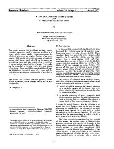
Computer Animation of the Sphere Eversion Nelson Max William H. Clifford, Jr. Case Western Reserve University The Sphere Eversion In 1948, Stephen Smale, a mathematician who was then at the University of Chicago, proved that it was possible to turn the surface of a sphere inside out by a special kind of deformation called a “regular homotopy”. During a regular homotopy, the surface must remain continuous, without any tears or holes, and smooth, without any creases or singularities. However, the surface is allowed to cross and pass through itself. In other words, if we consider a position of the sphere as a function from the standard round spherical surface S 2 into the three dimensional space R 3 , this function must be continuous and smooth (C1), but not necessarily one-to-one. Such a function is called an immersion, and some sample immersions of the sphere are shown in the figures here. A regular homotopy is then a continuous family of immersions, satisfying a technical condition that its partial derivatives with respect to position coordinates on S2 are continuous functions of time, as well as of position on S2. This is the smoothness condition which prohibits creases and kinks. Smale proved that there was a regular homotopy between any two immersions of the sphere. The ordinary round sphere and an inside-out round sphere are special cases of immersions, so there must be a regular homotopy between them. Smale’s proof was by induction and in principal contained a construction of an actual regular homotopy, but one so complicated that it would be impossible to visualize. Once the solution was known to be possible, a number of people tried to invent simple and easily visualized homotopies. One of these is discussed in a Scientific American article [7], which contains a more extensive description of the problem, and a complete sequence of illustrations for the homotopy. However, in order to understand the deformation, the reader must imagine the motions between the illustrations in the sequence, and convince himself that they are continuous and smooth. Clearly it would be preferable to have a movie showing the whole deformation. Since each frame is a different complicated surface, this is an obvious candidate for computer animation.
The film projected at the meeting and illustrated in the figures here shows a regular homotopy developed by Bernard Morin, a blind French mathematician who was also instrumental in the creation of several other such homotopies. The one used here is among the simplest known, since it contains only fourteen critical stages, the minimum among the homotopies known at present. There were two main problems in the creation of the film: first the mathematical definition of the homotopy to the computer, and second, the efficient computation of the frames for output through suitable hardware onto film. These will be discussed in the sections to follow.
Definition of the Surface The surface of the sphere was divided into eighteen rectangular and eight triangular patches, shown in Figure 1. For each patch, the three coordinates x, y, and z
Figure 1. Patches on the sphere. The exterior of the pattern is a final patch.
were represented as cubic polynomials in the two patch parameters u and v. Thus the rectangular patches were Coons’ “bicubic patches” [3], and the triangular ones were Birchoff’s “tricubic” patches [2]. The coefficients
for these polynomials were calculated from the coordinates of the vertices, the tangent vectors at the vertices, and the mixed partial derivative vectors, called the “twist vectors”. In order for two independent tangent vectors at a vertex to relate meaningfully to the partial derivatives for the patches having this vertex as a corner, each vertex must be a corner of four patches. Since it is impossible to cover a sphere using only rectangular patches which meet in this way, the triangular patches were needed. Since the rectangular patches are entirely determined by the tangent information at their vertices, they join automatically along their common edges to form a smooth continuous surface. After the program was written, Ed Catmull and Robert Barnhill at the University of Utah pointed out that the formulas for the triangular patches cause slight creases at their edges. However the smooth shading algorithm to be described later suppressed these creases anyway, so they were never corrected. The coordinate, tangent, and twist information to describe the surface involves more than 200 numbers, which must be specified for each position of the surface. However, each surface of the regular homotopy has two-fold rotational symmetry, visible in the symmetry of the patch structure in Figure 1. By taking advantage of this symmetry, the amount of information to describe each position is cut in half. In addition, the regular homotopy is symmetrical in time. At the halfway stage, shown in Figures 2 and 3, the inside surface and outside surface appear in identical positions, rotated by 90 degrees. The second half of the homotopy is a reversal of the first half with the inside and outside surfaces changing roles. Thus only half the homotopy need be specified.
Figure 3. Smooth surface rendering of halfway stage.
The vertex and tangent descriptions were entered interactively into a PDP-10 computer, using a program inspired by Andrew Armit’s “Multiobject” system [1] at Cambridge University. The original hope was to create the surfaces completely with this interactive program, comparing graphical output of the patches to a mental image of how the surfaces should look, and revising the data accordingly. However it was found that the surfaces were just too complicated for this to work well. One particularly annoying problem was the fact that a differentiable surface can nevertheless have a singularity, at a point where the two partial derivative vectors become linearly dependent. It is difficult to recognize how to modify the vertex and tangent information to eliminate these singularities.
Figure 4.
Figure 2. Wire frame network on halfway stage.
Luckily, a sequence of chicken-wire models for the homotopy had been constructed by Charles Pugh, at the University of California Berkeley (see Figure 4). Patches were
laid out on these models, and the necessary data was measured by hand, and entered into the computer. The interactive program was then ran at the Stanford Artificial Intelligence Laboratory, so that the data could be improved while the models were still accessible. This proved to be a much more satisfactory process, and we wish to thank Les Ernest for making the facilities at Stanford available. Since the de formation proceeds similarly forwards and backwards from the halfway position shown in Figures 2 and 3, the patches were chosen to fit best on this central surface, in the hope that they could be deformed both forward and backward to the beginning and final round spheres. However, this involved much twisting and distortion of the patches, and the surfaces resulting at the extremes of the homotopy had an unpleasant appearance. Therefore a completely different global representation, in terms of spherical coordinates, i.e., latitude and longitude, was employed for the beginning and final stages of the homotopy. Starting with the round sphere, trigonometric polynomials in the spherical coordinates were applied to push and twist the surface until it reached position S1, shown in Figure 5, approximating the model M1 of Figure 4 part way through the homotopy, where the patch representation takes over. In order to get a transition between the two representations, the patch surface P1 for M1 was also computed, and each patch subdivided into a number of small polygons, as shown in Figure 6. For each vertex of this subdivision, the spherical coordinates of the closest point on S1 were computed, using a metric which required nearness of the tangent planes as well as ordinary distance. In effect, this plastered the patch representation P1 onto the spherical coordinate surface, and once the crumpled parts of the surface were straightened out by hand, a smooth transition resulted.
Figure 6.
Each square patch was subdivided into a 6 by 6 array of smaller squares, shown on Figures 3 and 6 and the triangular and rectangular patches were divided similarly. For the global representation in terms of spherical coordinates, the sphere was subdivided onto a collection of triangles based on Buckminster Fuller’s geodesic dome (see [4]). The coordinates of the vertices of these subdivisions and of their “outward” surface normals were computed for a number of key frames and used as input for the shading process. The definition of these key frames was done at the Carnegie-Mellon University Computer Science Department and we wish to thank Raj Reddy for making the facilities there available to us.
Smooth Surface Representation
Figure 5.
The Evans and Sutherland LSD-2 animation machine at Case Western Reserve University was used to output the regular homotopy as a continuous family of smoothly shaded opaque surfaces. This machine takes as its input a sequence of polygon edges on the surface, and sends them through a pipeline where they are translated and rotated in a matrix multiplier, clipped on the screen edges, put into perspective, and stored in a sorted list. Then, a “Watkins box” [8] computes those segments of these polygons which are visible on each scan line, and a shader outputs the appropriate intensity signal at video rates. The shader computes the intensity by linearly interpolating the z component of the unit normal vectors at the vertices of the polygons. This piecewise linear intensity function approximates a cosine law of reflection as suggested by Gouraud [5].
found similarly. The profile curve EGF is then also approximated by a cubic, and intermediate points G, H, ... calculated, so that the polygon EFGH approximates the smooth profile curve, and the polygon AHCD is replaced by the two polygons AEGHFD and BEGHFC which can then be colored appropriately. The resulting smoothed profile is particularly beneficial when the surface is rotating or deforming, since otherwise vertices moving past the profile would cause temporary bumps to appear and disappear.
Figure 7.
If the subdivision into polygons is sufficiently fine, an apparently smoothly shaded surface results. However if two polygons meet at an edge with too sharp an angle, the eye, using contrast enhancement edge detection circuits in the retina, detects the discontinuity of the derivative of the piecewise linear shading and the edge shows as a bright “Mach band”, some of which are visible in Figure 7. There is also an anti-aliasing device on the pipeline, to eliminate the staircase effect produced on sharp edges by the finite resolution of the raster scan. The inside and outside surfaces of the sphere are colored in two contrasting colors, depending on whether the normal to the “outside” surface points toward or away from the viewer. To produce a segment of the movie, two key frame descriptions are stored in the PDP-11 computer which works with the LDS-2. These descriptions contain the positions and normals for corresponding vertices on the two surfaces, and a list of polygons which connect then. For each intermediate frame, the PDP-11 interpolates the data between the key frames, and sends it through the LDS-2. The only problem is with polygons which cross the profile curve, and thus have some vertex normals pointing towards the viewer, and some pointing away, making the decision as to color impossible. For each vertex the dot product of the vertex normal times the vector pointing from the vertex to the point of view is taken. These dot products are positive if the vertex is visible in the outside surface, and negative otherwise. An edge like AB connecting two points whose dot products have opposite signs is assumed to cross the profile curve at a point E. To find it, a weight is computed which would make the weighted average of the dot products for A and B come out zero. A cubic approximation to the curved side AEB of the patch is then formed using the normals at A and B to specify the curvature, and evaluated at the weight to find E. The point F is
Figure 8.
The LDS-2 is capable of continuously refreshing a fixed position of the surface for viewing with a 512 line raster, and is even capable of rotating it in real time if the dot product and profile smoothing computations are omitted. For high quality filming in color, three color filters are moved into place in turn under computer control, and a slower 1024 line high resolution scan is used. The computer also controls the advance of the film in the animation camera. We wish to thank Ted Glaser at Case Western Reserve University for making the LDS-2 available during the preparation of this paper. Once the key frames have been defined, the surfaces may be rotated, magnified, and filmed from any point of view, as in Figure 9. They can also be sliced by a clipping plane, to show the interior structure which would otherwise be obscured. As shown in Figure 10, this can be done on the LDS-2 hardware, which can clip with respect to a front and back plane, as well as on the screen boundaries. It can also be done in software, giving the smoother clipping edge shown in Figure 11, using methods analogous to those which produce a smooth profile edge. Another way to show the interior structure is to shrink the polygons on the surface, so that gaps appear between them, as shown in Figure 12, revealing the surfaces behind. A final way is to use a wire frame representation, as described below, which can be drawn on a vector scope.
diate frames, and the vectors are rotated and transformed into a display list suitable for the GDP. Only half the vectors need be kept in core, since the others can be obtained by rotation about the axis of two-fold symmetry of the surface.
Figure 9.
Fig. 11
Fig 10.
Wire Frame Representation The wire frame sequences in the film were made on a Graphics Display Processor (GDP), a high- speed digital vector scope, developed at Carnegie-Mellon University. Like the LDS-2, the GDP works in conjunction with a PDP-11, which can perform the interpolation between key frames, and in this case also does the matrix multiplication for the rotation. The screen has sixteen logarithmically spaced intensity levels, which are used to make the distant parts of the surface dimmer. For the animation, the two key frames are described in display lists, containing visible and invisible vectors in three dimensions. These are interpolated to form interme-
Figure 12
Two sorts of wire frame approximations were used: a cross hatching, suitable for the patch representation shown in Figures 2, 6, and 13 and a “chicken wire” array of hexagons, derived from the “geodesic” subdivision on the global representation, shown in Figures 5, 14 and 15. No attempt was made to provide a consistent representation throughout the deformation, since any pleasant looking
wire frame approximation to the round sphere would inevitably become unpleasantly distorted when the sphere was turned completely inside out. Instead, “live” film of the real chicken wire model M1 in Figure 4 was used to cover the transition. Note added to Siggraph ’95 Course Notes:
tion, and illustrates what may be accomplished in the future, in the direction of precise renderings of scientific phenomena.
The finished film actually did have the “unpleasantly distorted” cross hatch mesh showing the whole eversion.
Figure 15.
References Figure 13.
[1] Armit, A. P., “Multipatch and Multiobject Design Systems,” Proceedings Royal Society, London, A 321 (1971), p. 325. [2] Birchoff, G., “Tricubic Polynomial Interpolation,” Proc. Nat. Acad. Sci. USA, Vol. 68, No. 6, p. 1162 [3] Coons, S. A., Surfaces for Computer Aided Design of Space Forms, M.I.T. Project MAC TR-41 (1967). [4] Domebook 2, Shelter Publications, Salinas, California (1971). [5] Gouraud, H., Computer Display of Curved Surfaces, University of Utah, TUECH-CSC-70-101 (1970). [6] Max, N. L., “Computer Animation of Smooth Surfaces II,” Proc. 1973 “AIDE Meeting, available on microfiche from Nat’l. Microfilm Assoc.
Figure 14.
I believe the film provides a visualization which could not have been achieved in any other medium, and could never have been animated by hand. In fact, it is just at the borderline of what is now practical with computer anima-
[7] Phillips, A., “Turning a Sphere Inside Out,” Scientific American, Vol. 214, No. 5, (1966), p. 112. [8] Watkins, G. S., “A Real Time Visible Surface Algorithm,” Comp. Sci. Dept., U. of Utah, UTECH- CSC70-1 01 (1970).