COMPUTER SIMULATION OF MICROELECTRODE BASED BIO-IMPEDANCE MEASUREMENTS WITH COMSOL 1
Alberto Olmo1 and Alberto Yúfera2
Escuela Superior de Ingenieros (ESI), Dto. Física Aplicada III, Universidad de Sevilla Av. de los Descubrimientos s/n. 41092. Sevilla. Spain 2 Instituto de Microelectrónica de Sevilla (IMSE), Centro Nacional de Microelectrónica (CNM-CSIC) Universidad de Sevilla, Av. Américo Vespucio s/n. 41092. Sevilla. Spain
[email protected] ,
[email protected]
Keywords:
Microelectrode, Bioimpedance, Impedance sensor, Computer simulation, COMSOL.
Abstract:
Electrical models for microelectrode-cell interfaces are essential to match electrical simulations to real biosystems performance and correctly to decode the results obtained experimentally. The accurate response simulation of a microelectrode sensor to changes in the cell-electrode system, such as cell growth, enables the optimum microelectrode design process. We report the use of COMSOL quasi-static mode, contrary to other DC modes frequently used, including magnetic fields to calculate the bioimpedance of the system. A fully electrode-cell model has been built, and the effect of fibroblasts of different diameters on the simulated impedance of small microelectrodes (32-µm square) has been studied, in order to validate the model and to characterize the microelectrode sensor response to changes in cell size and density.
1
INTRODUCTION
Many biological parameters and processes can be sensed and monitored using its impedance as marker (Beach et al., 2005), (Yúfera et al., 2005), (Yúfera et al., 2008), (Radke and Alocilja, 2005), with the advantage of being a non-invasive and relatively cheap technique. Cell growth, changes in cell composition or changes in cell location are only some examples of processes which can be detected by microelectrode-cell impedance sensor variations. Electrical models have been reported for the electrode-cell interfaces (Huang et al., 2004), (Borkholder, 1998), (Joye et al, 2008), being these key for matching electrical simulations to real systems performance and hence decoding correctly the results obtained experimentally, usually known as reconstruction problem. Some of these models have been obtained by using the finite element analysis method with programs such as FEMLAB. (Huang et al., 2004). The use of the DC mode for a sinusoidal steady state calculation is possible by assigning a complex conductivity, which works because the Poisson equation is the same form as the Laplace equation in the charge-free domain. This paper presents an alternative method for simulating electrode – cell
178
interfaces with finite element analysis, based on COMSOL. The quasistatic mode of COMSOL is used, which also takes into account magnetic fields to calculate the electric impedance. Our work, based on previous models (Huang et al., 2004), is developed in section 2. Several improvements on their model have been made both on the cellular membrane and the cell-electrode gap, are described in section 3. Impedance changes on small electrodes (32- µm square) caused by different sizes of 3T3 mouse fibroblasts were simulated in section 4, in order to validate the model and characterize the microelectrode sensor response to cell growth. Finally, conclusions are highlighted in section 5.
2
CELL-ELECTRODE MODEL
The work performed by Huang et al. (Huang et al., 2004), was initially explored, making use of the computation advantages COMSOL provides over FEMLAB. Our objective is to compare the results in the study of the impedance changes caused by cell growth on electrodes with similar size to the cell. Cells modelled in the simulation by Huang et al. were 3T3 mouse fibroblasts, which attach closely to
COMPUTER SIMULATION OF MICROELECTRODE BASED BIO-IMPEDANCE MEASUREMENTS WITH COMSOL
surfaces and which have a cell-surface separation typically of 0.15µm (Giebel et al., 1999). The cells are about 5µm in height and, from a top view, are irregularly shaped and approximately 30–50µm in extent. A circular cell 30 µm in diameter centred on a square sensing electrode that is 32µm on each side was considered. (see figure 1). The sensing electrode was surrounded by a counter electrode that has considerably greater area. 3T3 mouse fibroblasts consist of a thin (about 8 nm), poorly conducting membrane that surrounds the highly conductive interior of the cell. The capacitance of the cell membrane is approximately Cmem = 1 µF/cm2 (Geddes, 1972). The cell culture medium simulated by Huang et al. is highly ionic and possesses a conductivity of approximately 1.5 S/m. The cell culture medium fills the cell-electrode gap and forms an electrical double layer (Helmholtz plus diffuse layer) between the bulk of the medium and the electrode that is approximately 2 nm in thickness. Some approximations were made in X. Huang´s work to facilitate the resolution of the problem by FEMLAB. Only one quarter of the electrode was simulated. As the problem is characterized by a wide range of distance scales, it was difficult to solve by finite-elements techniques, so the following adjustments were made: The electrical double layer modelling the electrode-solution equivalent circuit was replaced with a 0.5 µm thick region with the same specific contact impedance ⎡ (2π f )1/2
σ dl + j 2π f ε dl = t ⋅ ⎢ ⎣
Kw
+
⎤ j(2π f )1/2 + jC I 2π f ⎥ Kw ⎦
(1)
Where σdl and εdl are the conductivity and dielectric permittivity of the double layer, t is the thickness of the region, CI is the interfacial capacitance per unit area, which consists of the series combination of the Helmholtz double layer and the diffuse layer, and Kw is a constant related with Warburg impedance contribution. The cell membrane was replaced by a 0.5 µm thick region with the same capacitance per unit area
ε mem = t ⋅ Cmem
(2)
Where Cmem is the membrane capacitance per unit area and t = 0.5µm. Electrode-cell gap was replaced with a 0.5 µm thick region with the same sheet conductivity, that is
σ gap =
t cell −electrode ⋅ σ medium t
(3)
Where tcell-electrode is the gap thickness and t is again 0.5µm. In our work, the geometry of their simulation was adopted (see figure 1), and the values for the conductivity and permittivity of the electrical double layer were calculated following the same expression shown before (1), with the same values for Kw and CI mentioned in the article (Huang et al., 2004). Conductivity of the cell and the medium was also set to 1.5 S/m in our work. However, the model by X. Huang et al. for the electrode-cell gap and the cellular membrane (equations 2 and 3) was refined as shown in the following section.
Figure 1: Geometry of the model simulated in COMSOL.
3
MODEL ENHANCEMENT
Several modifications were made in the model in order to obtain simulations of cell impedance measurements with more accuracy and obtaining a more complex model that reflects real experiments in a more realistic way. Such modifications were made in the following areas:
3.1
Cellular Membrane
The equivalent circuit of the attached membrane was modelled as a resistance Rm in parallel with a capacitance Cm, in a similar way as reported by Joye et al. (Joye et al. 2008). These parameters are defined as Rm =
1 g mem ⋅ A
(4)
C m = cmem ⋅ A
Where A is the area of the attached membrane (in our case A=706.86e-12 m2), gmem = 0.3 mS/cm2 is the local membrane conductivity and cmem (1
179
BIODEVICES 2010 - International Conference on Biomedical Electronics and Devices
µF/cm2) is the membrane capacity per unit area (Joye et al. 2008). Making use of the following expression we can calculate the conductivity and permittivity of the cellular membrane from the impedance. Z=
1 K (σ + jωε )
(5)
Where K is the geometrical factor (K = area / length). In our case a value of 5 µm has been taken as the length. (This value corresponds to the thickness of the membrane layer represented in COMSOL). The value for K results 1413e-6, and the values obtained for conductivity and permittivity are σ =1.5e-6 S/m and ε = 5.001e-9 F/m (εr=565).
3.2
Cell Membrane-electrolyte Interface Capacitance
This capacitance was not considered in Huang´s model, but can also be important, as it models the charge region (also called the electrical double layer) which is created in the electrolyte at the interface with the cell. The capacitance Chd is defined as the series of three capacitances: Ch1 = Ch 2 = Cd =
ε 0ε IHP dIHP
Ace
ε 0ε OHP
dOHP − dIHP
q 2ε 0ε d KTz 2 n0 N KT
(6)
Ace Ace
Where Ace is the area of the attached membrane, ε0 is the dielectric permittivity of free space; εIHP and εOHP are respectively the Inner and Outer Helmholtz Plane relative dielectric constant; dIHP is the distance of the Inner Helmholtz Plane to the membrane; dOHP is the distance of the Outer Helmholtz Plane to the membrane; εd is the diffuse layer relative dielectric constant; KB is Boltzmann’s constant; T is the absolute temperature; q is the electron charge; z is the valence of ions in solution; n0 is the bulk concentration of ions in solution; and N is Avogadro’s number.
Comparing the impedance equivalent to this capacitance with the same expression as before (5), and modelling again this layer as a 5 µm thick layer with K =1413e-6, we obtained ε = 0.0011e-6 F/m, which corresponds to εr = 124.29, value that was inserted in COMSOL.
4
SIMULATION RESULTS WITH COMSOL
As can be seen in figure 1, only one quarter of the electrodes and cell was simulated. Electrodes were modelled with no thickness. The first layer modelled on top of the electrode surface is the electrical double layer, of 0.5 µm thickness, which can be seen in the figure. On top of the electrical double layer, the cell-electrode gap is modelled with another 0.5 µm layer. This layer includes in our simulation the cell membrane-electrolyte interface capacitance. On top of it we finally have the cell membrane, also modelled as another 0.5 µm layer, and the rest of the cell. For each layer, it is necessary to introduce in COMSOL the conductivity and permittivity values calculated before. All surfaces had an insulating boundary condition (n*J=0) with the exception of the surfaces separating the different layers and sub-domains within the model, which were set to continuity (n*(J1-J2) = 0) and the bottom surface of the two electrodes, which were set to an electric potential of 1V and 0V. The Quasi-statics module of COMSOL was used to perform the finite element simulations. In this mode, it is possible to obtain the solution for the electric potential for different frequencies. Simulations were performed on a 2.26 GHz Intel(R) Core(TM)2 DUO CPU. Solution times varied with the frequency but ranged from 3 to 6 minutes. In Figure 2 we can see the solution for the electric potential at the determined frequency of 100 Hz.
For Chd, the values given in Joye´s report (Joye et al. 2008) are considered. In particular, it is assumed that εIHP = 6, εOHP =32, dIHP = 0.3 nm, dOHP = 0.7 nm, z = 1, T = 300 K, and n0 =150 mM. The area of the attached membrane is in our case Ace=706.86e-12 m2. and εd is set to 1. The following values were obtained: Ch1= 0.125pF; Ch2=0.5pF; Cd=2.22pF And the total series capacitance was Chd=1.54pF.
180
Figure 2: Electric potential solution at 100Hz.
COMPUTER SIMULATION OF MICROELECTRODE BASED BIO-IMPEDANCE MEASUREMENTS WITH COMSOL
Two series of simulations, with frequency ranging from 102 Hz to 106 Hz, were made with and without the presence of the cell. Once the solution for the electric potential had been found by COMSOL, Boundary Integration was used to find the electric current through the counter electrode. With that value the electric impedance was calculated, taking into account that the voltage difference between electrodes was 1V and that impedance had to by divided by 4 (as only one quarter of the electrodes was simulated.) The values obtained are shown in figure 3.
other sizes of cell. Parameters of the cell membrane and cell membrane-electrolyte interface were recalculated for cells of 15 µm and 20 µm of diameter, inserted in COMSOL, and new simulations were performed. Results are also shown in figure 4.
Figure 4: Simulated normalized impedances of the system, for a 30µm-diameter cell (blue line), 20µm-diameter cell (magenta line) and 15µm-diameter cell (red line). Figure 3: Impedance magnitude of the microelectrode system with cell (red line) and without it (blue line).
The measured impedance changes by several orders of magnitude over the frequency range simulated, which is in accordance with previous works (Huang et al., 2004), (Borkholder, 1998). We can see how the presence of the cell changes the measured impedance, with the biggest change at a frequency near to 105 Hz. This is also in accordance with the report of Huang et al. Another way of representing the impedance magnitude is to observe the impedance changes of the system with cell on top respect to the microelectrode system without cell. This can be done by plotting the normalized impedance change, defined as Z − Z no.cell r = cell (7) Z no.cell Being Zcell and Zno.cell the impedance magnitudes with and without cell, respectively. The normalized impedance changes of the system with the 30µmdiameter cell modelled before is plotted in figure 4 (blue line). In order to have a measure of the system sensibility to changes in cell dimension, we repeated the calculations reported in sections 3.1 and 3.2 for
We observe how the system is sensitive to these differences in cell size. At the same frequency, the normalized impedance r increases with the cell dimension, being an excellent indicative of the area overlap between the microelectrode-cell and, allowing the measurement of the cell size and/or cell density. Normalized impedance peaks indicate the optimum frequency for measurements. It is of 0.03 for cells of 15 µm of diameter, and 0.14 for 30 µm of diameter at approximately 105 Hz. For cell density measurements, a fill factor parameter can be defined as a percentage of the microelectrode area covered by cells. These curves characterize the sensibility of the sensor and can be useful in the preliminary design of microelectrodes.
5
CONCLUSIONS
Electrical models for electrode-cell interfaces are the key for matching electrical simulations to real systems performance and correctly decoding the results obtained experimentally, usually known as reconstruction problem. They are also very useful to determine the sensibility of microelectrode sensors to different changes in processes such as cell growth.
181
BIODEVICES 2010 - International Conference on Biomedical Electronics and Devices
In our work, an enhance electrode-cell model was built, based on a previous work, incorporating the cellular membrane and the cell-electrode gap in order to obtain more accurately simulate impedance measurements. The quasi-static mode of COMSOL was used to perform the finite-element simulations. The influence of the cell size on the measured impedance of small electrodes (32-µm square) was studied, obtaining the greatest impedance changes due to the cell influence at frequencies near 105 Hz. The microelectrode sensor response to cell changes in growth was characterized. The model and finite element method simulation has proved to be a valid one, in agreement with other experimental results, which can be used in the future to simulate a wide number of biological experiments based on bio-impedance measurements and to characterize a large number of micro-sensors structures.
ACKNOWLEDGEMENTS We would like to thank Mrs. Josefa Guerrero, from the Physics Department of the University of Seville, for her valuable help with COMSOL simulations. This work is in part supported by the Spanish founded Project: TEC2007-68072, Técnicas para mejorar la calidad del test y las prestaciones del diseño en tecnologías CMOS submicrométricas.
REFERENCES Beach, R.D. et al, 2005. Towards a Miniature In Vivo Telemetry Monitoring System Dynamically Configurable as a Potentiostat or Galvanostat for Twoand Three- Electrode Biosensors, IEEE Trans. On Instrumentation and Measurement, vol. 54, nº1, pp: 61-72, 2005. Yúfera, A. et al., 2005. A Tissue Impedance Measurement Chip for Myocardial Ischemia Detection. IEEE Transaction on Circuits and Systems: Part I. vol.52, nº:12 pp: 2620-2628. Radke, S.M and Alocilja, E.C., 2004. Design and Fabrication of a Microimpedance Biosensor for Bacterial Detection, IEEE Sensor Journal, vol. 4, nº 4, pp: 434-440. Borkholder, D. A., 1998. Cell-Based Biosensors Using Microelectrodes. PhD Thesis, Stanford University. Huang X. et al., 2004. Simulation of Microelectrode Impedance Changes Due to Cell Growth, IEEE Sensors Journal, vol.4, nº5, pp: 576-583. Yúfera A. et al., 2008. A Method for Bioimpedance Measure with Four- and Two-Electrode Sensor
182
Systems, 30th Annual International IEEE EMBS Conference, pp: 2318-2321. Joye N. et al., 2008. An Electrical Model of the CellElectrode Interface for High-density Microelectrode Arrays, 30th Annual International IEEE EMBS Conference, pp: 559-562. 2008 Giebel, K.F. et al., 1999. Imaging of cell/substrate contacts of living cells with surface plasmon resonance microscopy, Biophysics Journal, vol. 76, pp: 509–516. Geddes, L.A., 1972. Electrodes and the Measurement of the Bioelectrical Events, New York. Wiley.