Constraint-Handling with Support Vector Decoders - Semantic Scholar

Constraint-Handling with Support Vector Decoders J¨org Bremer1 and Michael Sonnenschein1 University of Oldenburg, 26129 Oldenburg, Germany, {joerg.bremer|michael.sonnenschein}@uni-oldenburg.de

Abstract. A comparably new application for support vector machines is their use for meta-modeling the feasible region in constrained optimization problems. Applications have already been developed to optimization problems from the smart grid domain. Still, the problem of a standardized integration of such models into (evolutionary) optimization algorithms was as yet unsolved. We present a new decoder approach that constructs a mapping from the unit hyper cube to the feasible region from the learned support vector model. Thus, constrained problems are transferred into unconstrained ones by space mapping for easier search. We present result from artificial test cases as well as simulation results from smart grid use cases for real power planning scenarios. Keywords: smart grid, constraint-handling, decoder, constraint modeling, SVDD

1

Introduction

A popular class of commonly used heuristics for solving hard optimization problems is known as evolutionary search methods. These methods usually work with candidate solutions that encode each parameter within an allowed interval between a lower and an upper limit and try to improve them within these bounds. Thus, all solutions are defined in a d-dimensional hypercube. Nevertheless, due to additional constraints, not all of these solutions are usually feasible. Effectively solving real world optimization problems often suffers from the additional presence of constraints that have to be obeyed when exploring alternative solutions. Evolutionary algorithms have been widely noticed due to their potential for solving complex (discontinuous or non differentiable) numerical functions. However, a full success in the field of nonlinear programming problems is still missing, because constraints have not been addressed for integration in a systematic way [1, 2]. For constraint-handling, the general constrained continuous nonlinear programming (NLP) problem is often used as problem formulation: Find x ∈ Rd that optimizes f (x) subject to a set of constraints: equalities: gi (x) = 0; inequalities: g j (x) ≤ 0;

1≤i≤m 1 ≤ j ≤ n.

(1)

Real world problems often additionally face nonlinear constraints or such constraints that are not given as explicit formulation. One example for a not explicitly given constraint is a simulation model that devalues given solutions as not feasible judged by simulation runs. We are going to focus on (but not restrict ourselves to) the latter type.

In general, the set of constraints defines a region within a search space (the hypercube defined by parameter bounds) that contains all feasible solutions. Taking into account non-linear constraints, the NLP is generally intractable [1]. Evolutionary Algorithms approximately solve non linear optimization very efficiently. Nevertheless, surprisingly low effort has been put in the integration of constraint handling and evolutionary optimization (cf. [2]). Standard constraint-handling techniques are for example the introduction of a penalty for infeasible solutions, the separation of objectives and constraints to transform a given optimization problem into an unconstrained manyobjective one, or decoder approaches to give an algorithm hints on how to construct feasible solutions by imposing a relationship between feasibility and decoder solution. At the same time, support vector machines and related approaches have been shown to have excellent performance when trained as classifiers for multiple purposes, especially real world problems. In [3] a support vector model has been developed for the feasible region of an optimization problem specific to the smart grid domain. This model only allows for afterwards checking the feasibility of an already given solution. We integrate these two approaches to a new decoder approach for constraint handling [4]. Such a decoder is a constraint-handling technique that maps the constrained problem space to some other not-restricted space where the search operates. The basic idea is to construct a mapping from the original, unconstrained domain of the problem (the hypercube) to the feasible space. The mapping will be derived from the support vector model. After a brief review of constraint handling techniques and black-box modelling with support vector approaches, we introduce the underlying model and describe the construction of our mapping approach in detail. We present results from several test scenarios with artificial optimization problems and conclude with results from applying our method to the load balancing problem in smart grid scenarios.

2

Related Work

Several techniques for handling constraints are known. Nevertheless, many are concerned with special cases of NLP or require priori knowledge of the problem structure for proper adaption [1]. We will briefly discuss some prominent representatives of such techniques. A good overview can for instance be found in [5] or, more recently, in [2]. Penalty: A widely and long since used approach for constraint handling is the introduction of a penalty into the objective function that devalues all solutions that violate some constraint. In this way, the problem is transformed into an unconstrained one. Most commonly used are exterior penalties that draw outside solutions towards the feasible region in contrast to interior ones that keep solutions inside, but require to start with a feasible solution [5]. Separation of objectives and constraints: Constraints or aggregations of constraints may be treated as separate objectives. This leads to a transformation into a (unconstrained) many objective problem. Such approaches have some computational disadvantages from determining Pareto optimality or may lack the ability (in the case of a disjoint region) to escape a sub-region [5]. Moreover, a functional description of constraints must be known here in advance, what is not the case when using surrogate models that hide original relations and only model the original behaviour.

Solution repair: Some combinatorial optimization problem allow for an easy repair of infeasible solutions. In this case, it has been shown that repairing infeasible solutions often outperforms other approaches [6]. This approach is closely related to the decoder based approaches. Decoder: In order to give hints for solution construction, so called decoders impose a relationship between feasibility and decoder solutions. For example, [7] proposed a homomorphous mapping between an n-dimensional hyper cube and the feasible region in order to transform the problem into an topological equivalent one that is easier to handle, although with a need for extra parameters that have to be found empirically and with some extra computational efforts. In contrast, we will see later how a similar approach can be automatically derived from a given support vector description. Earlier approaches e.g. used Riemannien mapping [8]. A relatively new constraint handling technique is the use of meta-models for black-box optimization scenarios with no explicitly given constraint boundaries. Such a model allows for efficiently checking feasibility and thus eases the search for the constraint boundary between a feasible and an infeasible solution in case a repair of a mutation is needed. Various classification or regression methods might be harnessed for creating such models for the boundary [2]. An example from the smart grid for the latter case that has been realized by an SVDD approach can be found in [9] and is also an example for scenarios with (at least partly) unknown functional relationships of the constraints. When lacking full knowledge on hidden variables or intrinsic relations that determine the operability of a electric device, the feasible region can only be derived by sampling a simulation model [3]. The model is learned by SVDD from a set of operable (feasible) examples; in another example, [10] used a two-class SVM for learning operation point and bias (regarding allowed voltage and current bands) of a line in a power grid for easier classifying a grid state as feasible or not. In both cases, at the time of searching for the optimum, the only available information is the model, i.e. a set of support vectors and associated weights. Every information about the original constraints is no longer available in such scenarios. For our real world use case we will briefly review load balancing. Within the framework of today’s (centralized) operation planning for power stations, different heuristics are harnessed. Short-term scheduling of different generators assigns (in its classical interpretation) discrete-time-varying production levels to energy generators for a given planning horizon [11]. It is known to be an NP-hard problem [12]. Determining an exact global optimum is not possible in practice until ex post due to uncertainties and forecast errors. Additionally, it is hard to exchange operational constraints in case of a changed setting (e.g. a new composition of energy resources) of the generation system. Coordinating a pool of distributed generators and consumers with the intent to provide a certain aggregated load schedule for active power has some objective similarities to controlling a virtual power plant. Within the smart grid domain the volatile character of such a coalition has additionally to be taken into account. On an abstract level, approaches for controlling groups of distributed devices can be roughly divided into centralized and distributed scheduling algorithms. Centralized approaches have long time dominated the discussion [13] and are discussed in the context of static pools of energy unit with drawbacks and restrictions re-

garding scalability and particularly flexibility. Recently, distributed approaches gained more and more importance. Different works proposed hierarchical and decentralized architectures based on multi-agent systems and market based computing [14]. Newer approaches try to establish self-organization between actors within the grid [15, 16]. In load balancing scenarios, a scheduling algorithm (centralized or distributed) must know for each participating energy resource which load schedules are actually operable (satisfy all constraints) and which are not. Each energy resource has to restrict its possible operations due to several constraints. These can be distinguished into hard constraints (usually technically rooted, e.g. minimum and/or maximum power input or output) and soft constraints (often economically or ecologically rooted, e.g. personal preferences like noise pollution in the evening). When determining an optimal partition of the schedule for power production distribution, an alternative schedule is sought from each unit’s search space of individual operable schedules (individual feasible region) in order to assemble a desired aggregate load schedule.

3

Mapping Algorithm

We now describe the integration of a SVDD based black-box for feasible regions into an arbitrary evolutionary optimization algorithm with proper and effective constraint handling and propose handling constraints in a different way: by learning a mapping that transforms the original parameter hypercube to resemble the feasible region.

3.1

SVDD-Model for Feasible Regions

As a prerequisite for our mapping, we assume that the feasible region of an optimization problem has been encoded by SVDD as e.g. described in [9]. We will briefly describe this approach before deriving our new utilization method. Given a set of data samples xi ∈ X , the inherent structure of the region where the data resides in is derived as follows: After mapping the data to a high dimensional feature space, the smallest images enclosing sphere is determined. When mapping back the sphere to data space, its preimage forms a contour (not necessarily connected) enclosing the data sample. This task is achieved by determining a mapping Φ : X ⊂ Rd → H , x 7→ Φ(x) such that all data from a sample from a region X is mapped to a minimal hypersphere in some high-dimensional space H . The minimal sphere with radius RS and center a in H that encloses {Φ(xi )}N can be derived from minimizing kΦ(xi ) − ak2 ≤ R2 + ξi with k·k as the Euclidean norm and slack variables ξi ≥ 0 for soft constraints. After introducing Lagrangian multipliers and further relaxing to the Wolfe dual form, the well known Mercer’s theorem (cf. e.g. [17]) may be used for calculating dot products in H by means of a kernel in data space: Φ(xi ) · Φ(x j ) = k(xi , x j ). In order to gain a more smooth adaption, it is known to be advantageous to use a Gaus− 1 kx −x k2

sian kernel: kG (xi , x j ) = e 2σ2 i j [18]. SVDD delivers two main results: the center a = ∑i βi Φ(xi ) of the sphere in terms of an expansion into H and a function R : Rd → R that allows to determine the distance of the image of an arbitrary point from a ∈ H ,

calculated in Rd by: R2 (x) = 1 − 2 ∑ βi kG (xi , x) + ∑ βi β j kG (xi , x j ).

(2)

i, j

i

Because all support vectors are mapped right onto the surface of the sphere, the radius RS can be determined by the distance of an arbitrary support vector to the center a. Thus the feasible region is modeled as F = {x ∈ Rd |R(x) ≤ RS } ≈ X . This model might be used as a black-box that abstracts from any explicitly given form of constraints and allows for an easy and efficient decision on whether a given solution is feasible or not. Moreover, as the radius function Eq. 2 maps to R, it allows for a conclusion about how far away a solution is from feasibility. Nevertheless, a systematic constraint-handling during optimization is not induced in this way. In the following, we present a way of integrating such SVDD surrogate models into optimization. 3.2

The Decoder

Let F denote the feasible region within the parameter domain of some given optimization problem bounded by an associated set of constraints. It is known, that preprocessing the data by scaling it to [0, 1]d leads to better adaption [19]. For this reason, we consider optimization problems with scaled domains and denote with F[0,1] the likewise scaled region of feasible solutions. We construct a mapping γ : [0, 1]d → F[0,1] ⊆ [0, 1]d ; x 7→ γ(x)

(3)

that maps the unit hypercube [0, 1]d onto the d-dimensional region of feasible solutions. ˆ ` . Instead We achieve this mapping as a composition of three functions: γ = Φ{` 1 ◦ Γa ◦ Φ of trying to find a direct mapping to F[0,1] we go through kernel space. The commutative diagram (Eq. 4) sketches the idea. We start with an arbitrary point x ∈ [0, 1]d from the unconstrained d-dimensional hypercube and map it to an `-dimensional manifold that is spanned by the images of the ` support vectors. After drawing the mapped point to the sphere in order to pull it into the image of the feasible region, we search the pre-image of the modified image to get a point from F[0,1] . x ∈ [0, 1]d

ˆ` Φ

- Ψ ˆ x ∈ H (`)

γ

Γa

? x∗ ∈ F[0,1] ⊆ [0, 1]d 

? Φ{` 1

˜ x ∈ H (`) Ψ

(4)

Step 1: Mapping to the SV induced subspace H (`) with an empirical kernel map We will now have a closer look onto the respective steps of this procedure. Let Φ` : Rd → R` , x 7→ k(., x)|{s1,...,s` } = (k(s1 , x), . . . , k(s` , x))

(5)

be the empirical kernel map w.r.t. the set of support vectors {s1 , . . . , s` }. Then ˆ ` : Rd → H (`) , Φ

(6)

1

x 7→ K − 2 (k(s1 , x), . . . , k(s` , x))

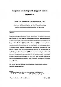
with Ki j = k(si , s j ): the kernel Gram Matrix, maps points x, y from input space to R` , ˆ ` (x) · Φ ˆ ` (y) (cf. [17]). With Φ ˆ ` we are able to map arbitrary points such that k(x, y) = Φ d (`) from [0, 1] to some `-dimensional space H that contains a lower dimensional projection of the sphere. Again, points from F[0,1] are mapped into or onto the projected sphere, outside points go outside the sphere (cf. fig. 1).

ˆx Ψ ˜x Ψ

x x∗

RS Rmax

Rd

H (`)

Fig. 1. Deriving the decoder from the support vector model.

Step 2: Re-adjustment in kernel space In general, in kernel space H the image of the region is represented as a hypersphere S with center a and radius RS (Eq. 2). Points outside this hypersphere are not images of points from X , i.e. in our case, points from F[0,1] are mapped (by Φ) into the sphere or onto its surface (support vectors), points from outside F[0,1] are mapped outside the sphere. Actually, using a Gaussian kernel, Φ maps each point into a n-dimensional manifold (with sample size n) embedded into infinite dimensional H . In principle, the same holds true for a lower dimensional embedding spanned by ` mapped support vectors and the `-dimensional projection of the hypersphere therein. We want to pull points from outside the feasible region into that region. As we do have rather a description of the image of the region, we draw images of outside points into the image of the region, i.e. into the hypersphere; precisely into its `-dimensional projection. For this purpose we use ˜ x = Γa (Ψ ˆ x) = Ψ ˆ x + µ · (a − Ψ ˆ x ) · Rx − RS Ψ Rx

(7)

ˆ x produced in step 1) into Ψ ˜x∈Φ ˆ x into ˆ ` (F[0,1] ) by drawing Ψ to transform the image Ψ the sphere. Alternatively, the simpler version ˆ ˜ x = a + (Ψx − a) · RS Ψ Rx

(8)

ˆ x just onto the sphere but then without having to estimate may be used for drawing Ψ parameter µ ∈ [1, Rx ]. Parameter µ allows us to control how far a point is drawn into the sphere (µ = 1 is equivalent to eq. 8, µ = Rx draws each point onto the center). If µ is set RS (compare Fig. 1), a larger sphere containing all images (including infeasible) is to Rmax rescaled onto the smaller one. In this way, each image is re-adjusted proportional to the original distance from the sphere and drawn into the direction of the center. Points from the interior are also moved under mapping γ in order to compensate for additional points coming from the exterior. In this way, the whole unit hypercube is literally squeezed to the form of the feasible region without a too large increasing of the density at the boundary. Though, if the feasible region is very small compared with the hypercube, density at the boundary increases (depending on the choice of µ). On the other hand, the likelihood of an optimum being at the boundary increases likewise. So, this might be a desired effect. ˜ x which is the image of a point from F[0,1] in terms After this procedure we have Ψ Γ a of a modified weight vector w˜ . Step 3: Finding an approximate pre-image As a last step, we have to find the pre˜ x in order to finally get the wanted mapping to F[0,1] . A major problem in image of Ψ determining the pre-image of a point from kernel space is that not every point from the span of Φ is the image of a mapped data point [17]. As we use a Gaussian kernel, none of our points from kernel space can be related to an exact pre-image except for trivial expansions with only one term [20]. For this reason, we will look for an approximate pre-image whose image lies closest to the given image using an iterative procedure after [21]. In our case (Gaussian kernel), we iterate x∗ to find the point closest to the pre-image and define approximation Φ{` 1 by equation ∗ 2

2

∑`i=1 (w˜ i a e−ksi −xn k /2σ si ) . ∗ 2 2 Γ ∑`i=1 (w˜ i a e−ksi −xn k /2σ ) Γ

∗ xn+1 =

(9)

As an initial guess for x0∗ we take the original point x and iterate it towards F[0,1] . As this procedure is sensitive to the choice of the starting point, it is important to have some fixed starting point in order to ensure determinism of the mapping. Empirically, x has showed up to be a useful guess. Finally, we have achieved our goal to map an arbitrary point from [0, 1]d into the region of feasible solutions described merely by a given set of support vectors and associated weights: xn∗ is the sought after image under mapping γ of x that lies in F[0,1] . We may use this decoder approach to transform constrained optimization problems into unconstrained ones by automatically constructing mapping γ from a SVDD model of the feasible region that has been learned from a set of feasible example solutions.

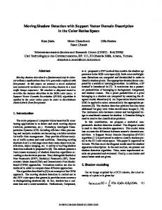
(a)

(b)

(c)

Fig. 2. 2(a): Sample from a artificial double banana shaped region. 2(b): Re-sampling the feasible region by mapping random points from [0, 1]2 . 2(c): marked optima of the Six-hump camel back objective function withing the used domain (depicted as heat map in the background).

4

Experiments

We present evaluation results of our decoder method with several theoretical test cases as well as results from the smart grid power planning problem. 4.1

General Test Cases

We started with several artificially constrained optimization problems and test functions. We consider optimization problems as described in section 1 and use the above described procedure as constraint handling technique, i.e. we transform problem Eq. 1 into an unconstrained optimization problem by applying mapping γ: optimize

f (γ(x)) , s.t. x ∈ [0, 1]d .

(10)

Of course, the restriction to the unit hypercube still entails a box constraint, but as these are easily handled by almost all algorithm implementations, this is not a serious obstacle. If x◦ ∈ [0, 1]d is the found position of the optimum in the unconstrained space then x˜ = γ(x◦ ) ∈ F[0,1] is the solution to the original, constrained problem. In the case of evolutionary algorithms, the method can be easily applied by defining the neighborhood in [0, 1]d and search the whole unit hypercube, but evaluate a solution x at the position γ(x). Note that mapping γ(x) generates a feasible solution regardless of the choice of x. Therefore optimization might always start with an arbitrary (randomly chosen) x ∈ [0, 1]d without having to find a feasible start solution first. For some first tests, we generated random samples from toy regions and used them as training sets. The retrieved support vectors and weights are taken as a model for feasible region F[0,1] . Figure 2(a) shows an example with a 2-dimensional double banana set. With these models, we constructed our mapping γ. As a first test, a set of 1 million equally distributed points has been randomly picked from [0, 1]2 and mapped. Figure 2(b) shows the result with mapped points.

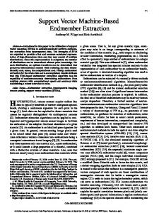
(a)

(b)

Fig. 3. 3(a): Randomly generated double ring data set as representation of a second toy region. Again, the orange line denotes the learned boundary that encloses the feasible space. 3(b): Mapping a mesh with grid size 0.02 into the learned region of a double ring data set.

Next, we applied standard particle swarm optimization (PSO) [22] and standard artificial bee colony (ABC) optimization [23] in order to find optima of several standard test objective functions. For this purpose, both algorithms have been equipped with mapping γ, while the topology of the neighbourhood that both algorithms operate on is defined as the whole unit hypercube. Figure 2(c) shows an example of found optima for the above sketched setting (both succeeded equally good). In this case, the well known Six-hump camel back function [24] has been used with the domain −1.9 ≤ x1 ≤ 1.9, −1.1 ≤ x2 ≤ 1.1 scaled to [0, 1]2 . As a second test case, double ring data sets (Figure 3(a)) have been generated. The contour plot in the background shows as objective Shubert’s function [25]. For the depicted configuration, different almost equally good local optima are situated near different distant positions at the boundary of the feasible region. Nevertheless, all algorithms equipped with mapping γ succeeded in finding optima inside (or at the boundary of) the feasible region. As a next step, we compared how fast a solution converges with a mapped objective function. We compared the performance, i.e. the speed of convergence, with exterior penalty approaches. Such a constraint handling approach entails additional penalty valTable 1. PSO and ABC and their absolute fitnesses (lower is better) after n iterations for the Shubert function as test function and double banana as constraint region.

A LGORITHM n

P ENALTY

M APPING

PSO

5 70.912 ± 89.714 -13.360±0.256 10 24.734 ± 68.949 -13.435±0.278 25 5.923 ± 47.904 -13.446±0.28 50 0.013 ± 41.368 -13.477±0.286

ABC

5 67.189 ± 89.783 -13.310±0.17 10 22.128 ± 64.272 -13.367±0.137 25 -2.897 ± 35.965 -13.496±0.175 50 -10.236 ± 15.765 -13.596±0.153

Table 2. Results for different objective functions and Algorithms. A double banana set has been used for all objectives. ABC: 87.98 and PSO: 83.22 percent were valid solutions for the penalty case; mapping: 100 percent.

BANANA O BJECTIVE

A LG .

S HUBERT S HUBERT S HUBERT S HUBERT B RANIN B RANIN Z AKHAROV Z AKHAROV B OHACHEVSKY 2 B OHACHEVSKY 2 B OHACHEVSKY 2 B OHACHEVSKY 2 H IMMELBLAU H IMMELBLAU

PSO 5 ABC 5 PSO 50 ABC 50 PSO 5 ABC 5 PSO 5 ABC 5 PSO 5 ABC 5 PSO 50 ABC 50 PSO 5 ABC 5

P ENALTY

M APPING

R INGS P ENALTY

-1.63 ± 38.95 -13.3 ± 0.41 -13.61 ± 9.02 -11.59 ± 8.35 -13.6 ± 0.35 -14.14 ± 0.49 -13.99 ± 0.06 -13.87 ± 0.13 -14.43 ± 0.0 -13.93 ± 0.08 -13.89 ± 0.01 -14.43 ± 0.0 135.39 ± 80.35 36.36 ± 0.91 43.61 ± 40.24 46.91 ± 33.78 36.15 ± 0.19 33.56 ± 1.73 1.54 ± 14.9 0.39 ± 0.08 0.18 ± 0.15 0.51 ± 3.9 0.38 ± 0.0 0.18 ± 0.08 0.93 ± 11.21 0.26 ± 0.1 0.43 ± 0.22 0.4 ± 2.76 0.24 ± 0.01 0.38 ± 0.11 0.24 ± 0.0 0.24 ± 0.0 0.27 ± 0.0 0.24 ± 0.01 0.24 ± 0.0 0.28 ± 0.01 179.84 ± 30.05 137.6 ± 1.96 127.11 ± 19.04 145.08 ± 14.38 136.03 ± 1.1 123.1 ± 1.69

M APPING -14.07 ± 0.75 -14.25 ± 0.22 -14.43 ± 0.01 -14.42 ± 0.01 33.14 ± 0.17 33.12 ± 0.02 0.14 ± 0.01 0.14 ± 0.0 0.32 ± 0.05 0.28 ± 0.02 0.27 ± 0.0 0.27 ± 0.0 121.84 ± 0.31 121.74 ± 0.06

ues to solutions outside the feasible region. According to [26], a penalty function that reflects the distances from the feasible region, is supposed to lead to better performance. Therefore, we have chosen the distance function of the SVDD (Eq. 2) as the penalty that attracts an outside solution to the feasible region. As we do not have any information on the original constraints, it is not in general possible to model penalties based on the number of or based on any individual constraint. Both algorithms converged faster with mapping than with penalty. The whole swarm operates completely inside the feasible region from the beginning when using a mapped objective function while retaining normal swarm behaviour in [0, 1]d . Tables 1 and 2 show further results. Table 1 focusses on the population size of swarm based approaches. Table 2 shows further results (the lower the better) on various combinations of algorithms and further objective functions for the case of the double banana dataset. Stated are respectively absolute achieved fitnesses, thus the ratio between mapping and penalty is to be compared. A major drawback of the penalty approach is the fact that it not always converges to a feasible solution. Whereas the mapping method

Fig. 4. A typical result for the speed of convergence in a higher dimensional test case; dashed: penalty approach.

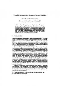
(a)

(b)

(c) Fig. 5. Results from a smart grid load balancing scenario with a standard penalty constrainthandling technique on the left (5(a)) and the mapping based approach on the right (5(b)); 5(c) compares the speed of convergence.

always served feasible solutions, the penalty approach failed in up to 17 percent of the test runs. Nevertheless, the inaccuracy inherent in the model from learning the region still remains an inaccuracy for mapping. But, the same holds true for all approaches that are based on such a surrogate model, including the penalty approach. Although, we made the observation that γ performs better at sharp edges than the decision boundary eq. 2 (cf. Figure 2(b)). Figure 3(b) shows the result of mapping a regular mesh from [0, 1]2 onto the double rings. The mapped mesh shows how points from different parts of the feasible region become neighbours under the γ by bypassing the infeasible region inside the rings. Figure 4 shows some results for test runs on an 8-dimensional problem with a stretched ellipse as feasible region and Himmelblau [27] as objective function. We compared artificial bee algorithms with 5 individuals for the mapping case and 200 individuals for the penalty case. Nevertheless, the mapping approach performs better and some penalty runs still converged to a infeasible solution, showing the superiority of the mapping approach. 4.2

The Smart Grid Use Case

Finally, we applied our method to the following real world problem from the smart grid domain: An individual schedule has to be determined for each member of a pool

of micro-co-generation (CHP) plants such that the aggregated electric load schedule of all plants resembles a given (probably demanded by market) target schedule in an optimal way. For the sake of simplicity, we will consider optimality as a close as possible adaption of the aggregated (sum of individual loads) schedule to the requested on. Optimality usually refers to additional local (individual cost) as well as to global (e.g. environmental impact) objectives. When determining an optimal partition of the schedule for load distribution, exactly one alternative schedule is taken from each generators search space of individual operable schedules in order to assemble the desired aggregate schedule. Therefore, the optimization problem is: finding any combination of schedules (one from each energy unit with Xi as the set of possible choices) that resembles the target schedule lT as close as possible, i.e. minimize some distance between aggregated and target schedule: k ∑ xi − lT k → min, s.t. xi ∈ Xi .

(11)

i

Of course, each generator has individual constraints such as time varying buffer charging, power ranges, minimum ON/ OFF times, etc. Thus, we simulated individual plants. For our simulations, we used simulation models of modulating CHP-plants (combined heat and power generator capable of varying the power level) with the following specification: Min. / max. electrical power: 1.3 / 4.7 kW, min. / max. thermal power: 4 / 12.5 kW; after shutting down, the device has to stay off for at least 2 hours. The relationship between electrical (active) power and thermal power was modeled after [28]. In order to gain enough degrees of freedom for varying active power, each CHP is equipped with an 800 litre thermal buffer store. Thermal energy consumption is modeled and simulated by a model of a detached house with its several heat losses (heater is supposed to keep the indoor temperature on a constant level) and randomized warm water drawing for gaining more diversity among the devices. For each simulated household, we implemented an agent capable of simulating the CHP (and surroundings and auxiliary devices) on a meso-scale level with energy flows among different model parts but no technical details. All simulations have so far been done with a time resolution of 15 minutes for different forecast horizons. Although, our method is indifferent about any such time constraints. We have run several test series with each CHP randomly initialized with different buffer charging levels, temperatures and water drawing profiles. The feasible spaces of individual CHP had been encoded with the SVDD approach. These support vector models have then been used for the search for optimal schedules: with a penalty approach on the one hand and with the proposed mapping on the other. Figure 5 shows a typical result. We used a co-variance matrix adaption evolution strategy (CMA-ES) approach [29] for finding combinations of schedules that best resemble the dashed target schedule in the top chart (Figures 5(a) and 5(b)). Both seem to have equally good results, but, looking at individual loads (in middle) and the temperatures (bottom) reveals that the penalty approach gets easily stuck at an (at least partly) infeasible solution whereas the mapping approach succeeds with feasible solutions. This effect amplifies with the number of plants and therefore with the number of used penalties. Moreover, the mapping approach most times converges faster as Figure 5(c) shows for this specific example.

Fig. 6. Power planning result with 750 micro co-generation plants. The top chart shows the target (dotted) as well as the achieved schedule. The load charts in the middle show the individual schedules of two types of chp in the group, the bottom chart shows resulting buffer temperatures. The grey bands denote allowed ranges of values.

Considering the complexity, additional computational costs are entailed on solution evaluation. Step 1 of the mapping growing quadratically with the number of support vectors ` is decisive together with the number of iterations necessary for finding the pre-image in step 3. Empirically, during our experiments, we observed for instance a mean number of iterations of 6.75 ± 0.3 for the case of the 2-dimensional double banana and 36.3 ± 26.4 for the case of a stretched 8-dimensional ellipse in order to reach convergence with 10−8 accuracy. Additionally, this number reduces in the course of optimization as soon as the evolution approaches feasible space. Otherwise, fewer function evaluations are necessary with our decoder approach, because we never evaluate infeasible solutions and we do not have to check feasibility during optimization. Both effects put into perspective the computational costs. Figure 6 shows an example from a scenario with 750 co-generation plants, demonstrating the ability to handle larger problems.

5

Conclusion

Many real world optimization problems face the effect of constraints that restrict the search space to an arbitrary shaped possibly disjoint region that contains the feasible solutions. Conventional constraint handling techniques often require the set of constraints to be a priori known and are hardly applicable for black-box models of feasible regions. Although penalties may be used with such models, the task of correctly tuning

the objective with these additional losses stays an error prone job due to the unknown nature of the original constraints that are no longer known at optimization time. We proposed a new constraint handling technique for support vector modeled search spaces and demonstrated its applicability and usefulness with the help of theoretical test problems as well as for a real world optimization problem taken from the smart grid domain. The major benefit of this approach is the universal applicability for problem transformation, solution repair and standardized integration in arbitrary evolutionary algorithms by constructing a modified objective function and treating the whole unconstrained domain as valid for search. So far, we have restricted ourselves to problems scaled to [0, 1]d . Further tests will show whether this limitation should be kept or whether arbitrary domains perform equally good.

Acknowledgement The Lower Saxony research network ’Smart Nord’ acknowledges the support of the Lower Saxony Ministry of Science and Culture through the Nieders¨achsisches Vorab grant programme (grant ZN 2764).

References 1. Michalewicz, Z., Schoenauer, M.: Evolutionary algorithms for constrained parameter optimization problems. Evol. Comput. 4 (March 1996) 1–32 2. Kramer, O.: A review of constraint-handling techniques for evolution strategies. Appl. Comp. Intell. Soft Comput. 2010 (January 2010) 3:1–3:19 3. Bremer, J., Rapp, B., Sonnenschein, M.: Support vector based encoding of distributed energy resources’ feasible load spaces. In: IEEE PES Conference on Innovative Smart Grid Technologies Europe, Chalmers Lindholmen, Gothenburg, Sweden (2010) 4. Bremer, J., Sonnenschein, M.: Constraint-handling for optimization with support vector surrogate models – a novel decoder approach. In Filipe, J., Fred, A., eds.: ICAART 2013 – Proceedings of the 5th International Conference on Agents and Artificial Intelligence. Volume 2., Barcelona, Spain, SciTePress (2013) 91–105 5. Coello Coello, C.A.: Theoretical and numerical constraint-handling techniques used with evolutionary algorithms: a survey of the state of the art. Computer Methods in Applied Mechanics and Engineering 191(11-12) (January 2002) 1245–1287 6. Liepins, G.E., Vose, M.D.: Representational issues in genetic optimization. Journal of Experimental and Theoretical Artificial Intelligence 2 (1990) 7. Koziel, S., Michalewicz, Z.: Evolutionary algorithms, homomorphous mappings, and constrained parameter optimization. Evol. Comput. 7 (March 1999) 19–44 8. Kim, D.G.: Riemann mapping based constraint handling for evolutionary search. In: SAC. (1998) 379–385 9. Bremer, J., Rapp, B., Sonnenschein, M.: Encoding distributed search spaces for virtual power plants. In: IEEE Symposium Series in Computational Intelligence 2011 (SSCI 2011), Paris, France (4 2011) 10. Blank, M., Gerwinn, S., Krause, O., Lehnhoff, S.: Support vector machines for an efficient representation of voltage band constraints. In: Innovative Smart Grid Technologies, IEEE PES (2011)

11. Pereira, J., Viana, A., Lucus, B., Matos, M.: A meta-heuristic approach to the unit commitment problem under network constraints. International Journal of Energy Sector Management 2(3) (2008) 449–467 12. Guan, X., Zhai, Q., Papalexopoulos, A.: Optimization based methods for unit commitment: Lagrangian relaxation versus general mixed integer programming. Volume 2. (2003) 1100 Vol. 2 13. Tr¨oschel, M., Appelrath, H.J.: Towards reactive scheduling for large-scale virtual power plants. In Braubach, L., van der Hoek, W., Petta, P., Pokahr, A., eds.: MATES. Volume 5774 of Lecture Notes in Computer Science., Springer (September 2009) 141–152 14. Kok, K., Derzsi, Z., Gordijn, J., Hommelberg, M., Warmer, C., Kamphuis, R., Akkermans, H.: Agent-based electricity balancing with distributed energy resources, a multiperspective case study. Hawaii International Conference on System Sciences 0 (2008) 173 15. Mihailescu, R.C., Vasirani, M., Ossowski, S.: Dynamic coalition adaptation for efficient agent-based virtual power plants. In: Proceedings of the 9th German conference on Multiagent system technologies. MATES’11, Berlin, Heidelberg, Springer-Verlag (2011) 101–112 16. Ramchurn, S.D., Vytelingum, P., Rogers, A., Jennings, N.R.: Agent-based control for decentralised demand side management in the smart grid. In Sonenberg, L., Stone, P., Tumer, K., Yolum, P., eds.: AAMAS, IFAAMAS (2011) 5–12 17. Sch¨olkopf, B., Mika, S., Burges, C., Knirsch, P., M¨uller, K.R., R¨atsch, G., Smola, A.: Input space vs. feature space in kernel-based methods. IEEE Transactions on Neural Networks 10(5) (1999) 1000–1017 18. Ben-Hur, A., Siegelmann, H.T., Horn, D., Vapnik, V.: Support vector clustering. Journal of Machine Learning Research 2 (2001) 125–137 19. Juszczak, P., Tax, D., Duin, R.P.W.: Feature scaling in support vector data description. In Deprettere, E., Belloum, A., Heijnsdijk, J., van der Stappen, F., eds.: Proc. ASCI 2002, 8th Annual Conf. of the Advanced School for Computing and Imaging. (2002) 95–102 20. Kwok, J., Tsang, I.: The pre-image problem in kernel methods. Neural Networks, IEEE Transactions on 15(6) (2004) 1517–1525 21. Mika, S., Sch¨olkopf, B., Smola, A., M¨uller, K.R., Scholz, M., R¨atsch, G.: Kernel PCA and de-noising in feature spaces. In: Proceedings of the 1998 conference on Advances in neural information processing systems II, Cambridge, MA, USA, MIT Press (1999) 536–542 22. Kennedy, J., Eberhart, R.: Particle swarm optimization. In: Neural Networks, 1995. Proceedings., IEEE International Conference on. Volume 4., IEEE (November 1995) 1942–1948 vol.4 23. Karaboga, D., Basturk, B.: A powerful and efficient algorithm for numerical function optimization: artificial bee colony (ABC) algorithm. Journal of Global Optimization 39(3) (November 2007) 459–471 24. Molga, M., Smutnicki, C.: Test functions for optimization needs. Technical report (2005) http://www.zsd.ict.pwr.wroc.pl/files/docs/functions.pdf. 25. Michalewicz, Z.: Genetic algorithms + data structures = evolution programs (3rd ed.). Springer-Verlag, London, UK (1996) 26. Richardson, J.T., Palmer, M.R., Liepins, G.E., Hilliard, M.R.: Some guidelines for genetic algorithms with penalty functions. In: Proceedings of the 3rd International Conference on Genetic Algorithms, San Francisco, CA, USA, Morgan Kaufmann Publishers Inc. (1989) 191–197 27. Himmelblau, D.: Applied nonlinear programming. McGraw-Hill (1972) 28. Thomas, B.: Mini-Blockheizkraftwerke: Grundlagen, Ger¨atetechnik, Betriebsdaten. Vogel Buchverlag (2007) 29. Hansen, N.: The CMA evolution strategy: a comparing review. In Lozano, J., Larranaga, P., Inza, I., Bengoetxea, E., eds.: Towards a new evolutionary computation. Advances on estimation of distribution algorithms. Springer (2006) 75–102