Indian Journal of Geo-Marine Sciences Vol. 40(2), April 2011, pp. 227-235
Data compression for underwater glider system using frequency sampling filters Rosmiwati Mohd-Mokhtar, Muhammad Hilmi R.A. Aziz, M. R. Arshad & Nur Afande Ali Hussain Underwater Robotic Research Group (URRG), School of Electrical and Electronic Engineering Universiti Sains Malaysia, Engineering Campus 14300 Nibong Tebal, Pulau Pinang, Malaysia [E-mail:
[email protected];
[email protected];
[email protected];
[email protected]] Received 23 March 2011, revised 28 April 2011 Data acquisition from underwater glider system yields large amounts of data. This may lead to a long computational time during the identification process. The raw data may also contain complex system disturbance information which may require a sophisticated optimization algorithm to achieve desirable results. In this paper, frequency sampling filters approach is used as a tool to compress the data and obtain meaningful parameter that describes the empirical model of the system. The use of finite impulse response model and the maximum likelihood method will play a role in eliminating the bias and noise effects of the glider data systems. By performing this procedure, the compressed, cleaned and unbiased data will be obtained, in which, it can be further used to develop a model of the glider system, also to analyze and observe for optimization and controller design purposes. [Keywords: Data compression, glider system, frequency sampling filters]
Introduction Autonomous underwater glider can be considered as one of the advanced prototype being designed in order to cope with the needs and requirement from ocean technology field. The underwater glider works based on buoyancy propulsion system and is designed to operate at low power consumption. It glides by controlling the buoyancy using internal tanks and pumps. Without using any thrusters or propellers, gliders are able to move upward and downward in a saw tooth pattern, turn and glide in a vertical spiral motion, only by changing the vehicle’s buoyancy intermittently. The idea of developing a glider was first inspired by Stommel in which in his article he stated that “A really new method was needed, one that would provide subsurface data on a scale and at a frequency that matched what remote sensing by satellite provided for the sea surface. Multiplying the number of ship by a factor of 100 was economically out of question.”1. Till 2001, three buoyancy driven autonomous underwater gliders have been developed. Doug Webb and his colleague via Webb Research Corporation have developed Slocum (named after Joshua Slocum, the New Englander who made his first single-handed global circumnavigation using his small sailboat)2, Scripps
Institution of Oceanography has developed Spray (named after Spray which is Joshua Slocum’s sailboat)3 and a University of Washington group has developed Seaglider4. There are two types of Slocum glider. The first type is electrically powered and able to operate for up to 200 meters depth using a syringe type ballast pump. The second type is thermally powered, which is able to operate for up to 1500 meters depth. Similar to Slocum Thermal, the Spray is also operated for up to 1500 meters depth. In the other hand, Seaglider can operate for up to 1000 meters depth only. Gliders are typically used in measurements of temperature, conductivity (to calculate salinity), currents, chlorophyll fluorescence, optical backscatter, bottom depth, and sometimes for acoustic backscatter of the ocean. Gliders can navigate through a periodic surface GPS fixes, pressure sensors, tilt sensors, and magnetic compasses. Ideally, the vehicle pitch is controllable by movable internal ballast (usually battery packs). The steering process is accomplished either with a rudder (as in Slocum) or by moving internal ballast to control roll (as in Spray and Seaglider). Buoyancy is adjusted either by using a piston in order to evacuate a compartment with seawater (Slocum) or by moving oil in/out of an external bladder (Seaglider, Spray, and Slocum Thermal).
228
INDIAN J. MAR. SCI., VOL. 40, NO. 2, APRIL 2011
Besides these three designs, there are also other outstanding glider design being developed, those are ALBAC at University of Tokyo5, STERNE at Ecole Nationale Superieure D’Ingenieurs (ENSIETA) in Brest, France6 and SeaExplorer which is also from a company in France. Although they share some of the similar features of Slocum, Spray and Seaglider, they are meant for different application and have some different features too. For example, instead of using a ballast system, the ALBAC glider is driven by a drop weight. In contrast, the STERNE is considered as a hybrid design since it has both ballast control and thrusters. As the positive demands and applicability of the underwater glider to do ocean sampling, the development of small-scale underwater glider is also carried out for experiment and research purposes. For example, the University of Princeton group has developed a small, laboratory-scale underwater glider called ROGUE (Remotely Operated Gliding Underwater Experiment)7. The same interest also runs at Universiti Sains Malaysia, in which here the research is conducted by the Underwater Robotic Research Group (URRG)8. The developed hull shape glider can be seen as in Fig. 1. Even though the development of the autonomous underwater glider technology has emerged more than a decade ago, there are still a lot of things that require for further enhancement and improvement of the system. Ranging from mechanical and environmental aspect to electronics and control system design, the issue on hydrodynamics, corrosion, ocean fluctuation, materials, stability, maintenance etc. are still open for research expand. By having the simulation and real prototype in the laboratory, analysis on design and development can be carried out extensively.
Fig. 1 Hull shape glider8
With respect to controller design of the underwater glider system, there are approximately ten state variables (representing the inter-relation of 10 dynamics) that need to be observed as to understand the vehicle behaviour. The analytical approach or physical modelling can be used to model the system. However, this kind of approach is somehow time consuming and require more laborious job and human resources. To deal with this situation, the empirical model obtained via system identification approach can be employed. System identification is based on study and analysis of the input and output data collected from the system. While performing this procedure, data acquisition process is unavoidable. Data acquisition process from real system typically yields large amounts of discrete-time data. This may lead to unacceptable computational time during the identification process. In addition, the raw data may contain complex system disturbance information which may require a sophisticated optimization algorithm in order to achieve desirable results. In reference to data collected from glider system, proper consideration has to be made since the glider system is very sensitive towards any change in sampling time. A slow sampling time leads to loss of information, while a fast sampling time tends to cluster the poles of the discrete time model near z = 1. It is shown that to obtain the inputs and outputs data, about 200,000 data sets are collected. This number is considered huge and may affect the identification time spend. Fortunately, this problem can be solved by introducing the frequency sampling filter within the first stage of the identification process. This stage is referred as data compression stage as the raw data will be analyzed in order to obtain only an important and meaningful parameter that describes the empirical model of the analyzed data. Based on the empirical model (parameterised by ), a continuous-time data suitable for identifying physical parameters is produced. By performing this procedure, the compressed, cleaned and unbiased step response and frequency response data will be obtained. The Frequency Sampling Filters (FSF) approach used in this paper is originally obtained from Wang and Cluett9-10. This approach involves the use of Finite Impulse Response (FIR) model and the maximum likelihood method which play a role in eliminating the bias and noise effects of the data
MOHD-MOKHTAR et al: DATA COMPRESSION FOR UNDERWATER GLIDER SYSTEM
collected from the systems. In order to obtain a proper FSF parameter optimization, the least squares model estimates based on PRESS (Predicted Residual Sum of Squares) computation is used11. This computation act to minimize the prediction error as well as determine the most suitable candidate for dynamic model structure. The idea of using FSF model for data compression is nothing new. It has been successfully applied for example in food extruder process12, Shell distillation column plant13, magnetic bearing system14-15 and during estimation of physical parameters of stable and unstable system16. However, the contribution of this paper is rather on the use of FSF model into the new real world application of underwater glider system. The introduction of this FSF model to the glider system will greatly benefit in terms of reducing the number of data to be used for system identification, eliminating the bias and noise effect that may occur and providing the significant parameter that may describe the empirical model of the glider true system. The remainder of this paper goes as follows. First section will explain about frequency sampling filter model. The step by step formulation will be delivered till the step response and the frequency response estimates are produced. The equations that are used in order to estimate the model using the PRESS criterion is also elaborated. Next, the result obtained from the FSF model will be demonstrated. The relevant discussion in regards to FSF model and the underwater glider system is also explained. Finally, a concluding remark is summarized in the conclusion section. Materials and Methods Frequency Sampling Filter Model
Introduce the FIR transfer function model as:
… (2) This time
relationship frequency
maps a set response
Where n is the model order chosen such that the FIR for all , and is the model coefficients backward shift operator. The model order n is determined from an estimate of the process settling and is the sampling time, , where interval10. Under the assumption that n is an odd number, the relationship between the process frequency response and its impulse response of the Inverse Discrete Fourier Transform (IDFT) is defined as:
of discrete coefficients,
into the set of discrete time unit impulse response coefficients, . Substituting Equation (2) into Equation (1) gives: ... (3)
The FSF approach approximates the transfer as16: function … (4)
… (5)
Where
are odd and the frequency sampling
interval, . is the m-th FSF and is the corresponding (complex) parameter (known as the maximum likelihood estimator). For the frequency gives an exact range of 0≤ω≤NΩ, choosing match
and choosing 9-10
... (1)
229
gives an
approximate match . The FSF filters are narrow band-limited around their respective centre frequencies. All the filters have identical frequency responses except for the location of their centre frequencies. Some of the FSF model characteristics are listed as below10. 1. FSF model only requires prior information about the process settling time expressed in terms of n. 2. The number of unknown parameters in the FSF model is equal to the number of unknown parameters in the FIR model. 3. FSF model corresponds to the discrete time frequency response coefficients. 4. The elements of the regressor vector for estimating the frequency response coefficients
INDIAN J. MAR. SCI., VOL. 40, NO. 2, APRIL 2011
230
are formed by passing the process input through the set of narrow band-limited frequency sampling filters. Fig. 2 shows the FSF model structure. The description of the system using frequency sampling filters is described as follows10.
Then, the estimate of solution given by
is obtained over least squares … (10)
which minimize the performance index of the form: … (11)
… (6) is the input signal, is the output where signal and is the disturbance signal. The FSF of Equation (4) can be rewritten in compact form as16: … (7) Where
In order to obtain a proper FSF parameter optimization, the least squares model estimates based on PRESS (Predicted Residual Sum of Squares) computation is used11. The PRESS criterion will ensure that the FSF model has the greatest predictive capability among all its candidate models. The PRESS Criterion
The idea of PRESS is to set aside each data point, estimate a model using the rest of the data, and then evaluate the prediction error at the point that was removed17. Instead of its usage in minimizing the prediction error, the PRESS statistic can be applied as a criterion for model structure detection in dynamic system identification11. The PRESS computation is originally based on the orthogonal decomposition algorithm proposed by Korenberg et.al.18.
Thus, Equation (6) can be rewritten as:
Define the prediction error as: … (8) For N data measurements, Equation (8) can also be written in matrix form as:
… (9)
e
-k(k)=y(k)-OtO(K)=y(k)-ý-k(k)-(12)
Where residuals and
are called the PRESS has been estimated according to
Equation (10) without including
Fig. 2 FSF model structure
and
. The
MOHD-MOKHTAR et al: DATA COMPRESSION FOR UNDERWATER GLIDER SYSTEM
PRESS residuals
represent the true prediction
errors, since and are independent. Based on the Shermon-Morrison-Woodbury theorem can be (see e.g. in17), the PRESS residuals calculated according to the following equation:
231
Substituting Equation (18) into (17), the estimated step response coefficient can be rewritten as:
… (19)
... (13) The PRESS statistic is defined as:
… (14) The average PRESS is calculated as:
Notice that the FSF approach is actually cast in the discrete time domain and the corresponding ztransform domain. However, the resultant model can be used to obtain continuous-time step response10. can be The system impulse response approximately computed using the continuous-time equivalent as:
… (15) Details regarding the computation of PRESS statistic can be referred in10.
… (20)
and
Step Response Estimation using FSF Model
In the estimation of step response, the description of the system using frequency sampling filters is described as follows. … (16)
… (21) where T is a sampling period. The step response is determined as: … (22)
Where for a suitable choice of and defined as in Equations (3) and (5), respectively. Upon obtaining the estimate of the frequency response parameters (according to FSF model and PRESS criterion), the estimate of the step response at sampling instant, n can be expressed by:
Frequency Response Estimation using FSF Model
The frequency response estimation is obtained over . Having say that, a transformation of Equations (4) and (5) can be rewritten in frequency domain form as:
… (17)
... (23)
where the estimated impulse response coefficients are related to frequency response via … (18)
… (24) Simulation of Equation of Motion
In order to study the underwater glider performance, a simulation prototype is first conducted
INDIAN J. MAR. SCI., VOL. 40, NO. 2, APRIL 2011
232
based on equation of motion restricted to vertical plane. As mentioned earlier, there are about ten state variables that need to be observed as to understand the underwater glider behaviour. Some of those are the glider’s depth, pitching angle, net buoyancy, angle of attack, velocity etc. In this paper, the equation of motion of an underwater glider as suggested by Leonard and Graver is used for simulation observation7. The equations are stated as follows: = =-
to the fixed body cord and MDL is the viscous moment. The forces and moment are modelled as: … (36) … (37)
… (25)
… (38)
… (26)
where the K’s are constant coefficients being defined as follows. ; ;
= Ωz
… (27)
; and
+MDL–rp3u1+rp1u3)
… (28)
The glider speed, V is denoted as: … (39)
… (29)
… (30) … (31)
… (32) … (33) … (34) … (35) Here, is the angle of attack, D is drag, L is lift, is pitching angle, v1 & v3 are the velocity with respect
A simulation of the equations of motion is performed using MATLAB software. The simulation of motion is conducted for a downward gliding motion for 50 seconds. In the downward gliding motion, the initial conditions of v1=0.3 sec, θ=-0.5 radians, mb=0, rp=0 and Ω=0 are used. The ballast rate acts as the control input for the simulation and some of the outputs such as depth, pitching angle and angle of attack are observed. The results show some of the hydrodynamic changes based on the input signal. Moreover, it is also important to know the control system of the buoyancy system itself. Therefore, the simulation was also conducted in an upward motion and the parameters (v1 , θ , mb , rp and Ω) were changed based on the push and pull of the ballast system. Results and Discussion Based on the simulation of the glider system, data acquisition process is conducted. A few sets of data are collected based on the observed glider dynamics. However, in this paper only 3 will be demonstrated
MOHD-MOKHTAR et al: DATA COMPRESSION FOR UNDERWATER GLIDER SYSTEM
that are the ballast rate-net buoyancy, ballast ratedepth and ballast rate-pitching angle data. The plot of input and output data of these three observed properties are shown as in Fig. 3, Fig. 4 and Fig. 5 respectively.
233
The number of actual raw data obtained from the simulation experiment and the number of data after the compression process is shown as in Table 1. Based on Table 1, it shows that the data have been successfully compressed to a better and significant number. The plot for step response and frequency response data after performing the FSF filters approach is demonstrated as in Fig. 6, Fig. 7 and Fig. 8 respectively.
Fig. 3 Input (ballast rate) & output (net buoyancy) data
Fig. 5 Input (ballast rate) & output (pitching angle) data Table 1 Number of data before and after performing FSF Types of data
Fig. 4 Input (ballast rate) & output (depth) data
Ballast rate – Net Buoyancy Ballast Rate – Depth Ballast Rate – Pitching Angle
Number of raw data
Number of compressed data
221938
2000
64784
1000
7000
1000
Fig. 6 The step response and the frequency response plot of the compressed data (ballast rate – net buoyancy data)
234
INDIAN J. MAR. SCI., VOL. 40, NO. 2, APRIL 2011
Fig. 7 The step response and the frequency response plot of the compressed data (ballast rate – depth data)
Fig. 8 The step response and the frequency response plot of the compressed data (ballast rate – pitching angle data)
As mentioned earlier, the underwater glider works based on buoyancy propulsion system, in which a concept of movable mass (shifting and changing mass) is employed. In order to maintain the robustness with respect to mass variations and other uncertainties, proper modeling and control design is necessary. With this significant reduced of number of data, the next step to obtain the model, to run the optimization process, to analyze the system in time domain and frequency domain or to gather information for controller design can be done conveniently. The less amounts of computational time and load (due to less number of data being process) will also help in improving the overall performance of those required procedures.
Conclusion The FSF approach is useful in assisting the problem of large amounts of data collected from underwater glider system. By performing the frequency sampling filters procedure, a compressed, cleaned and unbiased data of underwater glider system is obtained. The information gathered from this procedure can be further used to develop a model of the glider system. Besides that, analysis and observation can be done for optimization and controller design purposes. In addition, a validation test over real underwater glider data will also provide a significant meaning towards the actual system performance overall. This will be considered for the next research investigation in the near future.
MOHD-MOKHTAR et al: DATA COMPRESSION FOR UNDERWATER GLIDER SYSTEM
Acknowledgments Authors would like to thank University Sains Malaysia for the awarded short term grant (304/PELECT/6039034) to support this project.
9
10
References 1 Stommel, H. 1989.The Slocum mission. Oceanography, 2 (1): 22 – 25. 2 Webb, D. C., Simonetti, P. J. and Jones, C. P. 2001. Slocum: An underwater glider propelled by environmental energy, IEEE J. Oceanic Engineering, 26 (4): 447 – 452. 3 Sherman, R., Davis, E., Owens, W. B. and Valdes, J. 2001.The autonomous underwater glider Spray, IEEE J. Oceanic Engineering, 26 (4): 437 – 446. 4 Eriksen, C. C., Osse, T. J., Light, R. D., Wen, T., Lehman, T. W., Sabin, P. L, Ballard, J. W. and Chiodi, A. M. 2001. Seaglider: A long range autonomous underwater vehicle for oceanographic research. IEEE J. Oceanic Engineering, 26 (4): 424 – 436. 5 Tomoda, Y., Kawaguchi, K., Ura, T. and Kobayashi, H. 1993. Development and sea trials of a shuttle type AUV ALBAC. In Proc. of 8th Int. Symposium on Unmanned Untethered Submersible Tech., Durham, New Hampshire, 7 – 13. 6 Moitie, R. and Seube, N. 2001. Guidance and control of an autonomous underwater glider. In Proc. of 12th Int. Symposium on Unmanned Untethered Submersible Tech., Durham, New Hampshire, 14. 7 Leonard, N. E. and Graver. J. G. 2001. Model-based feedback control of autonomous underwater gliders. IEEE J. of Oceanic Engineering, Special Issue on Autonomous Ocean Sampling Networks, 26 (4): 633 – 645. 8 Ali-Hussain, N. A., Arshad, M. R. and Mohd-Mokhtar, R. 2009. Development of an underwater glider platform. 2nd
11 12
13
14
15
16
17 18
235
Postgraduate Colloquium School of Electrical & Electronic USM, EEPC 2009, Pulau Pinang, Malaysia. Wang, L. and Cluett, W. R. 1997. Frequency sampling filters: An improved model structure for step-response identification. Automatica, 33 (5): 939 – 944. Wang, L. and Cluett, W.R. 2000. From plant data to process control: Ideas for process identification and PID design. Francis & Taylor: London. Wang, L. and Cluett, W. R. 1996. Use of PRESS residuals in dynamic system identification. Automatica. 32: 781 – 784. Wang, L., Gawthrop, P. J. and Chessari, C. 2004. Indirect approach to continuous time system identification of food extruder. Journal of Process Control, 14 (6): 603 – 615. Arifin, N., Wang, L., Goberdhansingh, E. and Cluett, W.R. 1995. Identification of the Shell distillation column using the frequency sampling filter model. Journal of Process Control, 5: 71 – 76. Mohd-Mokhtar, R. and Wang, L. 2008. 2-stage approach for continuous time identification using step response estimates, In Proc. of IEEE Int. Conf. on System, Man & Cybernetics, Singapore, 3183 – 3188. Mohd-Mokhtar, R. and Wang, L. 2009. 2-stage identification based on frequency sampling filters and subspace frequency response, Elektrika: Journal of Electrical Engineering, 11(2): 27-33. Gawthrop, P. J. and Wang, L. 2005. Data compression for estimation of physical parameters of stable and unstable systems. Automatica, 41(8): 1313 – 1321. Myers, R.H. 1990. Classical and Modern Regression with Applications. 2nd ed. Duxbury Press: Boston. Korenberg, M., Billings, S.A., Liu, Y.P. and McIlroy, P.J. 1988. Orthogonal parameter estimation algorithm for nonlinear stochastic systems. Int. J. Control, 48(1): 193-210.