Data Pre-Processing Techniques for Classification ... - Semantic Scholar

Noname manuscript No. (will be inserted by the editor)

Data Pre-Processing Techniques for Classification without Discrimination Faisal Kamiran · Toon Calders

Received: date / Accepted: date

Abstract Recently the Discrimination-Aware Classification Problem has been proposed: given a situation in which our training data contains (e.g., gender or racial) discrimination, learn a classifier that optimizes accuracy, but does not discriminate in its predictions on the test data. Such situations occur naturally as artifacts of the data collection process when the training data is collected from different sources with different labeling criteria, when the data is generated by a biased decision process, or when the sensitive attribute serves as a proxy for unobserved features. In many situations, a classifier that detects and uses the racial or gender discrimination is undesirable for legal reasons. In this paper we survey and extend our existing data pre-processing techniques for removing discrimination from the input dataset after which the standard classifier inducers can be used. We propose three pre-processing techniques which are empirically validated, showing good performance on real-life census data. Keywords Classification · Discrimination-aware Data Mining

1 Introduction Classifier construction is one of the most researched topics within the data mining and machine learning communities. Literally thousands of algorithms have been proposed. The quality of the learned models, however, depends critically on the quality of the training data. No matter which classifier inducer is applied, if the training data is incorrect, poor models will result. In this paper we study cases in which the input data is discriminatory and we want to learn a discrimination-free classifier for future classification. Such cases naturally This paper is an extended version of the papers [14, 4, 15] F. Kamiran HG 7.46, P.O. Box 513, 5600 MB, Eindhoven, the Netherlands Tel.: +31-40-2475909 Fax: +123-40-2463992 E-mail: [email protected] T. Calders HG 7.82a, P.O. Box 513, 5600 MB, Eindhoven, the Netherlands

occur when, e.g., the decision process leading to the labels was biased due to discrimination as illustrated by the next example [4]. Throughout the years, an employment bureau recorded various parameters of job candidates. Based on these parameters, the company wants to learn a model for partially automating the match-making between a job and a job candidate. A match is labeled as successful if the company hires the applicant. It turns out, however, that the historical data is biased; for higher board functions, Caucasian males are systematically being favored. A model learned directly on this data will learn this discriminatory behavior and apply it over future predictions. From an ethical and legal point of view it is of course unacceptable that a model discriminating in this way is deployed. Next to data generated by a deliberately biased process, discrimination in training data also appears naturally when data is collected from different sources; e.g., surveys with subjective questions taken by different enquirers (leading, e.g., to an indirect discrimination based on the geographical area covered by enquirers), or when the sensitive attribute serves as a proxy of features that are not present in the dataset. With respect to this last case, we quote [23]: “If lenders think that race is a reliable proxy for factors they cannot easily observe that affect credit risk, they may have an economic incentive to discriminate against minorities. Thus, denying mortgage credit to a minority applicant on the basis of minorities on average-but not for the individual in question-may be economically rational. But it is still discrimination, and it is illegal.” In all these cases it is desirable to have a mean to “tell” the algorithm that it should not discriminate on basis of the attributes sex and ethnicity. Such attributes on which we do not want the classifier to base its predictions upon, we call sensitive attributes. Non-discriminatory Constraint. The original idea of discrimination-aware classification stems from [14,15]. We further explore the problem of discrimination in [4] where we concentrate on the case where a labeled dataset is given, and one binary attribute B which we do not want the predictions to correlate with. The dependency (discrimination) of the predictions of a classifier C on the binary attribute B with domain {b, b} is defined as ¡ ¢ ¡ ¢ P C =+|B =b −P C =+|B =b .

A discrimination larger than 0 reflects that a tuple for which B is b has a higher chance of being assigned the positive label by C than one where B is b. As showed before in our earlier works, simply removing the sensitive attributes is not sufficient to remove the discrimination, since other attributes may allow for determining the suppressed race or gender with high confidence. This we call the red-lining effect [14]. Solutions. The problem of classification with non-discriminatory constraints is in fact a multi-objective optimization problem; on the one hand the more discrimination we allow for, the higher accuracy we can obtain and on the other hand, in general we can trade in accuracy in order to reduce the discrimination. In the paper we start with a theoretical study of this trade-off. Then the following four methods for incorporating non-discriminatory constraints into the classifier construction process will be discussed. All four methods are based on pre-processing the data set after which the normal classification tools can be used. 1. Suppression. We find the most correlated attributes of the attribute B . To reduce the discrimination between the class labels and the attribute B , we simply remove B and its most correlated attributes. This simple and straightforward approach will serve as the base-line for our experiments. 2. Massaging the dataset. We change the labels of some objects in the dataset in order to remove the discrimination from the input data. A good selection of the objects to change is essential. To select the best candidates for relabeling, a ranker is used. On the cleaned

dataset the final classifier is learned. This method is an extension of the method proposed in [14] where only a Naive Bayesian classifier was considered for both the ranking and learning. In this paper we consider arbitrary combinations of ranker and learner. 3. Reweighing. Instead of changing the labels, the tuples in the training dataset are assigned weights. As we will show, by carefully choosing the weights, the training dataset can be balanced w.r.t. B without having to change any of the labels. Many classification methods are based on frequencies. In these methods the weights can be used directly in the frequency counts, leading to non-discriminating classifiers. This method was first proposed in [4]. 4. Sampling. In Sampling we calculate the sample size for all combinations of B - and Class -values to make the dataset discrimination-free. We introduce two sampling techniques to change the original sample size to newly calculated one. In the first sampling scheme, simply we do random sampling with replacement to change the sample size. In this scheme, every object has a uniform probability to be duplicated to increase the sample size or to be skipped to decrease the sample size. We refer this sampling scheme to Uniform Sampling (US). In the second sampling scheme, border line objects get high priority for being duplicated or being skipped. We refer this sampling scheme to Preferential Sampling (PS). Experiments. A thorough empirical study was conducted. In the paper we present the results of experiments supporting the following claims: (i) The redlining effect is indeed present; removing the attribute B from the dataset does not always result in the removal of the discrimination. (ii) Especially the Massaging and PS techniques lead to an effective decrease in discrimination with a minimal loss in accuracy. (iii) Learning a classifier with non-discriminatory constraints can lead to more accurate classifier when only the training data and not the test-data contains the undesired discrimination. Contributions: The contributions of this paper can be summarized as follows: – The theoretical study of non-discriminatory constraints for classification and the discriminationaccuracy trade-off. – Previously proposed solutions are extended and are compared to each other. – Sanity check. In some of our experiments we learn a classifier on discriminatory training data and test it over non discriminatory data. For this purpose we use the census data from the Netherlands in the 70s as training set and the census data of 2001 as test set. In these 30 years, gender discrimination w.r.t. unemployment decreased considerably which provides us an opportunity for assessing the quality of a classifier learned on biased data on (nearly) discrimination-free data. The results of these experiments show that the discrimination-aware methods do not only outperform the traditional classification methods w.r.t. discrimination, but also w.r.t. predictive accuracy. – Extensive experimental studies show that our proposed solutions lead to discriminationfree future decision making by maintaining high accuracy. The results reported in this paper are empirically evaluated over multiple datasets. Outline. The rest of the paper is organized as follows. The motivation for the discrimination problem is given in Section 2. In Section 3 we formally define the problem statement and make a theoretical analysis of the trade-off between accuracy and discrimination. In Section 4, the three different approaches towards the problem are discussed. These solutions are empirically evaluated in Section 5 and Section 6 describes related work. Section 7 concludes the paper and gives directions for further work.

2 Motivation and Redlining Discrimination refers to the unfair and unequal treatment of individuals of a certain group based solely on their affiliation to that particular group, category or class. Such discriminatory attitude deprives the members of one group from the benefits and opportunities which are accessible to other groups. Different forms of discrimination in employment, income, education, finance and in many other social activities may be based on age, gender, skin color, religion, race, language, culture, marital status, economic condition etc. Such discriminatory practices are usually fueled by stereotypes, an exaggerated or distorted belief about a group. Discrimination is often socially, ethically and legally unacceptable and may lead to conflicts among different groups. Many anti-discrimination laws, e.g., the Australian Sex Discrimination Act 1984 [1], the US Equal Pay Act of 1963 and the US Equal Credit opportunity act [2] have been enacted to eradicate the discrimination and prejudices. However, if we are interested to apply classification techniques, and our available historical data contains discrimination, to the knowledge extraction process and decision making, it will be illegal to use traditional classifiers without taking the discrimination aspect into count due to these anti-discrimination laws. Due to the above mentioned laws or simply due to ethical concerns such use of existing classification techniques is unacceptable. Such a situation leads to the development of non-discriminatory classification techniques. We want to learn these non-discriminatory classification models from the potentially biased historical data such that they generate accurate predictions for future decision making yet does not discriminate with respect to a given discriminatory attribute. As illustrated by the next example, the use of non-discriminatory constraints in data mining can be applied to many other real world problems: A survey is being conducted by a team of researchers; each researcher visits a number of regionally co-located hospitals and enquires some patients. The survey contains ambiguous questions (e.g., “Is the patient anxious?”, “Is the patient suffering from delusions?”). Different enquirers will answer to these questions in different ways. Generalizing directly from the training set consisting of all surveys without taking into account these differences among the enquirers may easily result in misleading findings. For example, if many surveys from hospitals in area A are supplied by an enquirer who more quickly than the others diagnoses anxiety symptoms, faulty conclusions such as “Patients in area A suffer from anxiety symptoms more often than other patients” may emerge. Whereas in the job-candidate matching example in the introduction the data was correct (the label reflected whether someone did or did not get the job) and the non-discriminatory constraints were useful from a utility point of view, in the hospital survey example the non-discriminatory constraints are a useful tool to avoid overfitting the classifier to artifacts by requiring that the learned classifier does not correlate with the enquirer. Redlining: The problem of classification with non-discriminatory constraints is not a trivial one. The straightforward solution of removing the attribute B from the trainingset does in most cases not solve this problem at all. Consider, for example, the German Dataset available in the UCI ML-repository [3]. This dataset contains demographic information of people applying for loans and the outcome of the scoring procedure. The rating in this dataset correlates with the age of the applicant. Removing the age attribute from the data, however, does not remove the age-discrimination, as many other attributes such as, e.g., own house, indicating if the applicant is a home-owner, turn out to be good predictors for age. Similarly removing the sex and ethnicity for the job-matching example or enquirer for the survey example from the training data often does not solve this, as other attributes

may be correlated with the suppressed attributes. For example, area can be highly correlated with enquirer. Blindly applying an out-of-the-box classifier on the medical-survey data without the enquirer attribute may still lead to a model that discriminates indirectly based on the locality of the hospital. A parallel can be drawn with the practice of redlining: denying inhabitants of certain racially determined areas from services such as loans. It describes the practice of marking a red line on a map to delineate the area where banks would not invest; later the term was applied to discrimination against a particular group of people (usually by race or sex) no matter the geography. During the heyday of redlining, the areas most frequently discriminated against were black inner city neighborhoods. Through at least the 1990s this practice meant that banks would often lend to lower income whites but not to middle or upper income blacks1 , i.e., the decisions of banks were discriminatory towards black loan applicants. We further explore this impact of redlining over some dataset which we use in our experiments. Table 1 shows the results of experiments in which we lean traditional decision tree over the four datasets. We observe that just removal of discriminatory attribute does not solve the problem because the leaned model still discriminates due to the redlining effect.

Table 1 Redlining and different datasets. Dataset German Credit Census Income Communities and Crimes Dutch 2001 Census

With Disc Att 11.09% 16.48% 40.14% 34.91%

Without Disc Att 9.32% 16.65% 38.07% 17.92%

In many cases the discrimination can be explained; e.g., it may very well be that females in an employment dataset overall have lower levels of education than males, justifying a correlation between the gender and the class label. Nevertheless, in this paper we assume this not to be the case. We assume that the data is already divided up into strata based on acceptable explanatory attributes. As such, within a stratum (e.g., all people with same education level), gender discrimination can no longer be justified. A recently started collaboration with WODC, the study center of the Dutch Department of Justice and CBS, the Dutch central bureau of statistics is an important source of motivation to study the problem of discrimination. These agencies support policy making on the basis of demographic and crime information they have. Their interest emerges from the possibility of correlations between ethnicity and criminality that can only be partially explained by other attributes due to data incompleteness (e.g., latent factors). Learning models and classifiers directly on such data could lead to discriminatory recommendations to the decision makers. Removing the ethnicity attributes would not solve the problem due to the red-lining effect, but rather aggravate it, as the discrimination still would be present, only it would be better hidden. In such situations our discrimination-aware data mining paradigm clearly applies.

1

Source: http://en.wikipedia.org/wiki/Redlining, October 20th, 2009

3 Problem Statement In this section we formally introduce the notion of a non-discriminatory constraint and we theoretically analyze the trade-off between accuracy and discrimination. 3.1 Non-discriminatory Constraints We assume a set of attributes A = {A1 , . . . , An } and their respective domains dom (Ai ), i = 1 . . . n have been given. A tuple over the schema (A1 , . . . , An ) is an element of dom (A1 ) × . . . × dom (An ). A dataset over the schema (A1 , . . . , An ) is a finite set of such tuples and a labeled dataset is a finite set of tuples over the schema (A1 , . . . , An , Class ). Throughout the paper we will assume dom (Class) = {−, +}. We assume that a special attribute B ∈ A, called the sensitive attribute, and a special value b ∈ dom (B ), called the deprived community have been given. The semantics of B and b is that they define the discriminated community; e.g., B = Ethnicity and b = Black . For reasons of simplicity we will assume that the domain of B is binary; i.e., dom(B ) = {b, b}. Obviously, we can easily transform a dataset with multiple attribute values for B into a binary one by replacing all values v ∈ dom (B ) \ {b} with a new dedicated value b. We do not want the classifier to base its predictions upon the sensitive attribute, e.g., gender,religion. Let a labeled database D, an attribute B and a value b ∈ dom (B ) be given. We define the discrimination in the following way: Definition 1 (Discrimination): The discrimination in D, disc B =b (D), is defined as the difference of the probability of being in the positive class between the tuples having B = b in D and those having B 6= b in D; that is: disc B =b (D) :=

|{x ∈ D | x(B ) = b, x(Class ) = +}| |{x ∈ D | x(B ) = b}| −

|{x ∈ D | x(B ) = b, x(Class ) = +}| . |{x ∈ D | x(B ) = b}|

(When clear from the context we will omit B = b from the subscript.) A positive discrimination means that tuples with B = b are less likely to be in the positive class than tuples with B = b. Example 1 In Table 2, an example dataset is given. This dataset contains the Sex, Ethnicity, Highest Degree of 10 job applicants, the Job Type they applied for and the Class defining the outcome of the selection procedure. In this dataset, the discrimination w.r.t. the attribute Sex and Class will be disc Sex =f (D) := 45 − 25 = 40% . It means that the data object with Sex = f will have 40% less chance of getting a job than the one with Sex = m. Our way of measuring discrimination as the difference in positive class probability between the two groups is based upon the following observation. Suppose we have data on employees that applied for jobs and whether or not they gort the job and we want to test if there is gender discrimination. Therefore, we consider the proportion of men that were hired versus the proportion of women that were hired. A statistically significant difference in these proportions would indicate discrimination. Let us indicate the true (resp. observed) proportion of males receiving a high salary as m1 (x1 ), and the proportion for the females

Table 2 Sample relation for the job-application example. Sex

Ethnicity

m m m m m f f f f f

native native native non-nat. non-nat. non-nat. native native non-nat. native

Highest Degree h. school univ. h. school h. school univ. univ. h. school none univ. h. school

Job Type

Class

board board board healthcare healthcare education education healthcare education board

+ + + + + +

as m2 (x2 ). Notice that our discrimination measure equals x1 − x2 . The standard statistical approach for testing if females are discriminated would be to test if a one-sided test null hypothesis h0 : m2 ≥ m1 can be rejected. If the hypothesis gets rejected, the probability is high that there is discrimination. Many different statistical tests could be used in this example; popular tests that apply are, among others, a two-sample t-test, or a two-proportion Z-test. Besides trying to refute the null hypothesis h0 , we could also go for a test of independence between the attributes gender and class with, e.g., a χ2 -test or a G-test. Unfortunately there is no single best test; depending on the situation (usually depending on the absence or presence of abundant data or of the proportions taking extreme values) one test may be preferable over another. Here we can reasonably assume, however, since we are working in a data mining context, that sufficient data is available. We also assume that none of the proportions takes extreme values. As such, the choice of test is not that important, as long as we restrict ourselves to one test. The test-statistic that would be used for a two-sample t-test (assuming unknown and potentially different variances) is: disc gender =f x − x2 q 12 = q 2 , 2 2 s1 n1

+

s2 n2

s1 n1

+

s2 n2

where s1 and s2 denote the empirical standard deviations of the two groups and n1 and n2 their respective sizes. The statistical test, however, only tells us if there is discrimination, but does not indicate the severity of discrimination. In this respect notice that the test statistic for the hypothesis h0 : m1 − m2 = d0 is: x1 − x2 − d0 q 2 . 2 s1 n1

+

s2 n2

As this example shows, it is not unreasonable to take the difference between proportions as a measure for the severity of discrimination. Nevertheless, we want to emphasize that similar arguments can be found for defining the discrimination as a ratio, or for using measures based on mutual information gain between sensitive attribute and class or entropy-based measures (such as the G-test). In our work we made the choice for the difference in proportions because, statistically speaking, it makes sense, and it has the advantage of having a clear and intuitive meaning of expressing the magnitude of the observed discrimination.

3.2 Classifying with Non-discriminatory Constraints The problem we study in the paper is now as follows: Definition 2 Classifier with non-discriminatory constraint: Given a labeled dataset D an attribute B , and a value b ∈ dom (B ), learn a classifier C such that: (a) the accuracy of C for future predictions is high; and (b) the discrimination w.r.t. B = b is low. Clearly there will be a trade-off between the accuracy and the discrimination of the classifier. In general, lowering the discrimination will result in lowering the accuracy as well and vice versa. This trade-off is further elaborated upon in the next subsection. In this paper we are making three strong assumptions: A1 We are implicitly assuming that the primary intention is learning the most accurate classifier for which the discrimination is 0. When we assume the labels result from a biased process, insisting on high accuracy may be debatable. Nevertheless, any alternative would imply making assumptions on which objects are more likely to have been mislabeled. Such assumptions would introduce an unacceptable bias in the evaluation of the algorithms towards favoring those that are based on these assumptions. In the case where the labels are correct, yet the discrimination comes from the the sensitive attribute being a proxy for absent features, optimizing accuracy is clearly the right thing to do. A2 Ideally the learned classifier should not use the attribute B to make its predictions but we also present a scenario when the attribute B is used for classifier learning and for making future predictions. Knowing the attribute B at prediction time may lead to socalled “positive discrimination” to cancel out the discrimination, which is not always desirable when one can be held legally accountable for decisions based on the classifier’s predictions. Besides, it is contradictory to explicitly use the sensitive attribute in decision making while the goal is exactly to ensure that decisions do not depend on the sensitive attribute. A3 The total ratio of positive predictions of the learned classifier should be similar to the ratio of positive labels in the dataset D. This assumption would hold, e.g., when assigning a positive label to a person implies an action for which resources are limited; e.g., a bank that can assign only a limited number of loans or a university having bounded capacity for admitting students. We do not claim that other settings where these assumptions are violated are not of interest, but at the current stage our work is restricted to these settings.

3.3 Accuracy - discrimination Trade-Off Before going into the proposed solutions, we first theoretically study the trade-off between discrimination and accuracy in a general setting. Definition 3 We will call a classifier optimal w.r.t. discrimination and accuracy (DA-optimal) in a set of classifiers C if it is an element of that class and there does not exist another classifier in that class C with at the same time a lower discrimination and a higher accuracy. ∗ Perfect Classifiers. We will use Call to denote the set of all classifiers and Call to denote the set of all classifiers such that P (C (x) = +) = P (x(Class ) = +). Suppose that we have

a labeled dataset D and the perfect classifier P for this dataset; that is, P (x) = x(Class ) for all x ∈ D. P is an optimal classifier w.r.t. accuracy. Let D0 and D1 be defined as follows: D0 := {x ∈ D | x(B ) = b} D1 := {x ∈ D | x(B ) = b}

and let d0 and d1 be respectively |D0 |/|D| and |D1 |/|D|. The following theorem gives us some insight in the trade-off between accuracy and discrimination in perfect classifiers, namely those that are DA-optimal in the set of all classifiers, and those that are DA-optimal in the set of all classifiers that does not change the class distribution: Theorem 1 A classifier C is DA-optimal in Call iff acc (C ) = 1 − min(d0 , d1 )(disc (P ) − disc (C )) ∗ A classifier C is DA-optimal in Call iff

acc (C ) = 1 − 2d0 d1 (disc (P ) − disc (C ))

Proof sketch for Theorem 1. We denote the set of true negatives, true positives, false positives and false negatives of C by respectively TN , TP , FP , and FN . Their relative sizes | will be denoted tn , tp , fp , fn respectively. That is: tn = |TN . We also consider the split of |D| D into D0 = {t ∈ D | t.D = 0} and D1 = {t ∈ D | t.D = 1}, and denote the relative frac0| 1| 0| tions d0 = |D and d1 = |D . Similarly, TN 0 will denote D0 ∩ TN , and tn 0 = |TN . |D| |D| |D0 | With these conventions, we can express the accuracy and discrimination of C as follows: acc (C ) = tp + tn = d0 (tp 0 + tn 0 ) + d1 (tp 1 + tn 1 ) disc (C ) = (tp 0 + fp 0 ) − (tp 1 + fp 1 )

A careful analysis of these formulas reveals that any DA-optimal classifier must have fp 0 and fn 1 equal to 0. Furthermore, accuracy can be lowered while keeping disc (C ) constant by decreasing tn 0 by ² and increasing tp 1 at the same time by the same amount ². The effect of this is that acc (C ) increases or decreases depending on the relative magnitudes of d0 and d1 . Depending on which choice increases acc (c), either tn 0 is maximized or minimized leading to the given bounds. ¤ As was claimed before, there is a trade-off between the accuracy of the DA-optimal classifiers and their discrimination. This trade-off is linear; lowering the discrimination level by 1% results in an accuracy decrease of min(d0 , d1 )% and an accuracy decrease of 2d0 d1 % if the class distribution needs to be maintained. These DA-optimal classifiers can be constructed from the perfect classifier. Imperfect Classifiers. Of course in reality we never have a perfect classifier to start from. From any given classifier C , however, we can easily construct a (non-deterministic) classifier by changing the predicted labels. For a given tuple x, C [p0+ , p0− , p1+ , p1− ] will assign the label C (x) with probability px(B )x(Class) and the other label with probability 1 − px(B )x(Class) . That is, pbc represents the probability that the label assigned by C to a tuple with B = b and Class = c will remain the same in the new classifier. Notice that the accuracy and discrimination of this random classifier in fact represents the expected accuracy and discrimination of all deterministic classifiers with p0+ , p0− , p1+ , p1− correspondence with C . We will denote the class of all classifiers that can be derived from C in ∗ this way by CC . CC will denote all classifiers C 0 in CC for which it holds that P (C 0 (x) = +) = P (C (x) = +) The following theorem characterizes the DA-optimal classifiers of CC ∗ and of CC .

Theorem 2 The classifier C 0 is DA-optimal in CC iff acc (C ) − acc (C 0 ) = α(disc (C ) − disc (C 0 )) ³ ´ tn 1 −fn 1 0 −fp 0 with α := min d0 tp , d . 1 tp +fp tn 1 +fn 0

0

1

∗ The classifier C 0 is DA-optimal in CC iff

h

acc (C ) − acc (C 0 ) = β (disc (C ) − disc (C 0 )) i

tn 1 −fn 1 0 −fp 0 with β := d0 d1 tp tp 0 +fp 0 + tn 1 +fn 1 . tp i (tn i ,fp i ,fn i ), i = 0, 1 denotes the true positive (true negative, false positive, false negative) rate in Di .

Proof sketch for Theorem 2. For the classifier C 0 , the true positive rate for D0 , tp 00 , is: tp 00 = p0+ tp 0 + (1 − p0− )fn 0 , as there are two types of true positive predictions: on the one hand true positive predictions of C and that were not changed in C 0 (probability po+ ) and on the other hand false negative predictions of C that were changed in C 0 (probability 1 −p0− ). For the other quantities similar identities exist. Using the same naming conventions as in the proof of Theorem 1, we now get: acc (C 0 ) = d0 (tp 00 + tn 00 ) + d1 (tp 01 + tn 01 )

= d0 (p0+ tp 0 + (1 − p0− )fn 0 + p0− tn 0 + (1 − p0+ )fp 0 ) + d1 (p1+ tp 1 + (1 − p1− )fn 1 + p1− tn 1 + (1 − p1+ )fp 1 ) 0

disc (C ) = (tp 01 + fp 01 ) − (tp 00 + fp 00 )

= (p1+ tp 1 + (1 − p1− )fn 1 + p1+ fp 1 + (1 − p1− )tn 1 ) − (p0+ tp 0 + (1 − p0− )fn 0 + p0+ fp 0 + (1 − p0− )tn 0 )

Similarly as in the proof of Theorem 1, we can show that for a DA-optimal classifier, p0+ = p1− = 1; i.e., we never change a positive prediction in D0 to a negative one or a negative prediction in D1 into a positive one. Depending on the exact true and false positive and negative rates and the sizes d0 and d1 , the optimal solutions are as given in the theorem. ¤

Again we see a linear trade-off. This linear trade-off could be interpreted as bad news: no matter what we do, we will always have to trade in accuracy proportional to the decrease in discrimination we want to achieve. Especially when the classes are balanced this is a high price to pay. Classifiers based on rankers. On the bright side, however, most classification models actually provide a score or probability for each tuple for being in the positive class instead of only giving the class label. This score allows us for a more careful choice of for which tuples to change the predicted label: instead of using a uniform weight for all tuples with the same predicted class and B -value the score can be used as follows. We dynamically set different cut-off c0 and c1 for respectively tuples with B = 0 and B = 1; for a ranker R, the classifier R(c0 , c1 ) will predict + for a tuple x if x(B ) = 0 and R(x) ≥ c0 , or x(B ) = 1 and R(x) ≥ c1 . Otherwise − is predicted. The class of all classifiers R(c0 , c1 ) will be denoted CR . Intuitively one expects that slight changes to the discrimination will only incur minimal changes to the accuracy, as the tuples that are being changed are the least certain ones and hence actually sometimes a change will result in a better accuracy. The decrease in accuracy will thus no longer be linear in the change in discrimination, but its rate will increase as the change in discrimination increases, until in the end it becomes linear again, because the

J48

86

IB3

82.5 82.0

85

81.5

84

Accuracy

Accuracy

81.0

83

80.5 80.0 79.5 79.0

82

78.5 81 0

2

4

6

8

10

Dependence

14

12

78.0 0

16

(a) Decision tree - AUC=73%

5

10

15

Dependence

20

25

(b) IBk - AUC = 80% NBS

83.5 83.0 82.5

Accuracy

82.0 81.5 81.0 80.5 80.0 79.5 79.0 0

5

10

15

Dependence

20

25

30

(c) Naive Bayes - AUC = 84% Fig. 1 Trade-off between accuracy and discrimination (dependence) for the DA-optimal classifiers in CR and CC .

tuples we change will become increasingly more certain leading to a case similar to that of the perfect classifier. A full analytical exposition of this case, however, is far beyond the scope of this paper. Instead we tested this trade-off empirically. The results of this study are shown in Figure 1. In this figure the DA-optimal classifiers in the classes CR (curves) and C (straight line) are shown for the Census-Income dataset [3]. The three classifiers are a Decision Tree (J48), a 3-Nearest Neighbor model (3NN), and a Naive Bayesian Classifier (NBS). The ranking versions are obtained from respectively the (training) class distribution in the leaves, a distance-weighted average of the labels of the 3 nearest neighbors, and the posterior probability score. The classifiers based on the scores perform considerably better than those based on the classifier only. Conclusion. In this section the accuracy-discrimination trade-off is clearly illustrated. It is theoretically shown that if we rely on classifiers, and not on rankers, the best we can hope for is a linear trade-off between accuracy and discrimination. For important classes of classifiers the DA-optimal classifiers were explicitly constructed. Notice, however, that the theoretical solutions proposed in this section violate our assumption A2; the classifiers C [p0+ , p0− , p1+ , p1− ] and R(c0 , c1 ) heavily use the attribute B to make their predictions. Therefore these optimal solutions are not suitable for our purposes. In the next section three solutions will be proposed that do not make use of the attribute B at prediction time, but only in the learning phase. The theoretically optimal solutions proposed in this section can be seen as “top-lines” which in theory we cannot outperform (without B we have strictly less information and hence, if our learning methods would be perfect, our model of the dis-

tribution that generated the data deteriorates). It represents the goal that we want to approach as close as possible.

4 Solutions: Data Preprocessing Techniques In this section we propose three solutions to learn a non-discriminating classifier that uses the attribute B only during learning not at prediction time. All solutions are based on removing the discrimination from the training dataset. On this cleaned dataset then a classifier can be learned. Our rationale for this approach is that, since the classifier is trained on discrimination-free data, it is likely that its predictions will be (more) discrimination-free as well. The empirical evaluation in Section 5 will confirm this statement. The first approach we present, called Massaging the data, is based on changing the class labels in order to remove the discrimination from the training data. A preliminary version of this approach was presented in [14]. The second approach is less intrusive as it does not change the class labels. Instead, weights are assigned to the data objects to make the dataset discriminationfree. This approach will be called Reweighing. Since reweighing requires the learner to be able to work with weighted tuples, we also propose a third solution in which we re-sample the dataset in such a way that the discrimination is removed. We will refer to this approach as Sampling. Two ways of sampling will be presented and tested.

4.1 Massaging In Massaging, we will change the labels of some objects x with x(B ) = b from − to +, and the same number of objects with x(B ) = b is changed from + to −. In this way the discrimination decreases, yet the overall class distribution is maintained. From the proof of Theorem 1 we know that this strategy reduces the discrimination to the desirable level with the least number of changes to the dataset while keeping the overall class distribution fixed. The set pr of objects x with x(B ) = b and x(Class) = − will be called the promotion candidates and the set dem of objects x with x(B ) = b and x(Class) = + will be called the demotion candidates. We will not randomly pick promotion and demotion candidates to relabel. Instead a ranker will be used to select the best tuples as follows. We assume the ranker assigns a score (higher is more positive) based on which examples can be ranked. On the training data, a ranker R for ranking the object according to their positive class probability is learned. With this ranker, the promotion candidates are sorted according to descending score by R and the demotion candidates according to ascending score. When selecting promotion and demotion candidates, first the top elements will be chosen. In this way, the objects closest to the decision border are selected first to be relabeled, leading to a minimal effect on the accuracy. The modification of the training data is continued until the discrimination in it becomes zero. The number M of modifications required to make the data discriminationfree can be calculated by using the following formula: M =

(b × (b ∧ +)) − (b × (b ∧ +)) b+b

where b and b represent respectively the number of objects with B = b and B 6= b while b∧ + and b∧ + are the number of objects of class + such that B = b and B 6= b, respectively.

Table 3 Sample job-application relation with positive class probability. Sex

Ethnicity

m m m m m f f f f f



Job Type

Cl.

Prob


+ + + + + +

98% 89% 98% 69% 30% 2% 40% 76% 2% 93%

Table 4 Promotion candidates (negative objects with Sex = f in descending order) and demotion candidates (positive objects with Sex = m in ascending order) Sex

Ethnicity

f f f

native non-nat. non-nat.

Sex

Ethnicity

m m m m

non-nat. native native native

Highest Degree h. school univ. univ. Highest Degree h. school univ. h. school h. school

Job Type

Cl.

Prob

education education education

-

40% 2% 2%

Job Type

Cl.

Prob

healthcare board board board

+ + + +

69% 89% 98% 98%

Example 2 Consider again the example Table 2. We want to learn a classifier to predict the class of objects for which the predictions are non-discriminatory towards Sex = f . In this example we rank the objects by their positive class probability given by a Naive Bayesian classification model. In Table 3 the positive class probabilities as given by this ranker are added to the table for reference (calculated by using NBS implementation of Weka). In the second step, we arrange the data separately for female applicant with class − in descending order and for male applicants with class + in ascending order with respect to their positive class probability. The ordered promotion and demotion candidates are given in Table 4. The number M of labels of promotion and demotion candidates we need to change equals: (f × (m ∧ +)) − (m × (f ∧ +)) f +m (5 × 4) − (5 × 2) = 1 = 5 +5

M =

So, one change from the promotion candidates list and one change from the demotion candidates list will be required to make the data discrimination-free. We change the labels of the top promotion and demotion candidates (rows highlighted with the bold font in Table 4). After the labels for these instances are changed, the discrimination will decrease from 40% to 0%. So, the dataset (which will be used for future classifier learning) becomes discrimination-free. ¤

Algorithm 1: Changing the Class Labels 1 Input (D, B, b, +) 2 Output Classifier learnt on D without discrimination

1: 2: 3: 4: 5: 6: 7: 8: 9: 10: 11: 12:

(pr , dem) := Rank (D, B, b, +) existDisc := DiscB=b (D) Calculate M , the number of necessary modifications based on existDisc for M times do Select the data object from the top of pr Change the class label of the selected object in D Select the data object from the top of dem Change the class label of the selected object in D Remove the top elements of both pr and dem end for Train a classifier on the modified D return Classifier with Non-discriminatory Constraint

Algorithm 2: Rank 1 Input (D, B, b, +) 2 Output (pr , dem): Two ordered lists of data objects on the basis of target class probability.

1: 2: 3: 4: 5:

Learn a ranker R based on D Calculate the class probabilities R(x) for all x ∈ D Add all x in D with x(B) = b and x(c) 6= + into the list pr in descending order w.r.t. R(x) Add all x in D with x(B) = b and x(c) = + into the list dem in ascending order w.r.t. R(x) return (pr , dem)

Algorithm. The pseudocode of our algorithm is given in Algorithm 1 and Algorithm 2. Algorithm 1 describes the approach of changing the class labels and classifier learning, and Algorithm 2 the process of ordering the data objects separately for the promotion and demotion lists.

4.2 Reweighing The Massaging approach is rather intrusive as it changes the labels of the objects. Our second approach does not have this disadvantage. Instead of relabeling the objects, different weights will be attached to them. For example, objects with B = b and Class = + will get higher weights than objects with B = b and Class = − and objects with B = b and Class = + will get lower weights than objects with B = b and Class = −. We will refer to this method as Reweighing. Again we assume that we want to reduce the discrimination to 0 while maintaining the overall positive class probability. We discuss the idea of weight calculation by recalling some basic notions of probability theory with respect to this particular problem setting. If the dataset D is unbiased, in the sense that B and Class are independent of each other, the expected probability Pexp (b ∧ +) would be: Pexp (b ∧ +) := b × +

where b is the fraction of objects having B = b and + the fraction of tuples having Class = +. In reality, however, the actual probability Pact (b ∧ +) := b ∧ +

Table 5 Sample job-application relation with weights. Sex

Ethnicity

m m m m m f f f f f



Job Type

Cl.


+ + + + + +

Weight 0.75 0.75 0.75 0.75 2 0.67 0.67 1.5 0.67 1.5

might be different where b ∧ + represents the fraction of data objects with B = b and Class = +. If the expected probability is higher than the actual probability value, it shows the bias towards class − for B = b. We will assign weights to b with respect to class +. The weight will be Pexp (b ∧ +) W (x(B ) = b | x(Class ) = +) := . Pact (b ∧ +) This weight of b for class + will increase the importance of objects with B = b for the class +. The weight of b for class − will be W (x(B ) = b | x(Class ) = −) :=

Pexp (b ∧ −) Pact (b ∧ −)

and the weights of b for class + and − will be W (x(B ) = b | x(Class ) = +) :=

Pexp (b ∧ +) Pact (b ∧ +)

W (x(B ) = b | x(Class ) = −) :=

Pexp (b ∧ −) . Pact (b ∧ −)

In this way we assign a weight to every tuple according to its B - and Class -values. The dataset with these weights becomes balanced. On this balanced dataset the discriminationfree classifier is learned. Example 3 Consider again the database in Table 2. The weight for each data object is computed according to its B - and Class -value. We calculate the weight of a data object with B = f and Class + as follows. We know that 50% objects have B = f and 60% objects have Class -value +, so the expected probability of the object should be: Pexp (Sex = f | x(Class ) = +) = 0 .5 × 0 .6

but its actual probability is 20%. So the weight W will be: W (Sex = f | x(Class ) = +) =

0.5 × 0.6 = 1 .5 . 0.2

Similarly the weights of the other combinations are: W (Sex = f | x(Class ) = −) = 0.67 W (Sex = m | x(Class ) = +) = 0.75 W (Sex = m | x(Class ) = −) = 2 .

Algorithm 3: Reweighing 1 Input (D, B, Class) 2 Output Classifier learnt on D without discrimination

1: 2: 3: 4: 5: 6: 7:

wtlist := Weights(D, B, Class) for All data objects in D do Select the value v of B and c of Class for the current data object Get the weight W from wtlist for this combination of v and c and assign W to the data object. end for Train a classifier on the balanced D return Classifier with Non-discriminatory Constraint

Algorithm 4: Weights 1 Input (D, B, Class) 2 Output The list of weights for each combination of B- and Class-values.

1: for All vi ∈ B do for All cj ∈ C do 2: 3: Calculate expected probability Pexp (vi ∧ cj ) = P (vi ) × P (cj ) in D 4: Calculate actual probability Pact (vi ∧ cj ) = P (vi ∧ cj ) in D 5: Weight W for the data object with B = vi and Class = cj will be 6: Add W, vi and cj in wtlist end for 7: 8: end for 9: return wtlist

Pexp (vi ∧cj ) Pact (vi ∧cj

The weight of each data object of the Table 2 is given in Table 5. Algorithm. The pseudocode of the algorithm describing our Reweighing approach is given in Algorithm 3 and Algorithm 4 describes the procedure of weight calculation.

4.3 Sampling Since not all classifier learners can directly incorporate weights in their learning process, we also propose a Sampling approach. In this way, the dataset with weights is transformed into a normal dataset which can be used by all algorithms. By sampling the objects with replacement according to the weights, we make the given dataset discrimination-free. We partition the dataset into four groups: DP (Deprived community with P ositive class labels), DN (Deprived community with N egative class labels), FP (F avored community with P ositive class labels), and FN (F avored community with N egative class labels): DP := {x ∈ D | x(B ) = b ∧ x(Class ) = +} DN := {x ∈ D | x(B ) = b ∧ x(Class ) = −} FP := {x ∈ D | x(B ) = b ∧ x(Class ) = +} FN := {x ∈ D | x(B ) = b ∧ x(Class ) = −}.

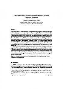
Consider the conceptual representation of an example dataset in Figure 2, showing 40 data points. The data points in the positive class are represented by +, the data points of the

Fig. 2 A figure with 40 data points.

negative class by −. The horizontal axis shows the probability of each data object to be in the positive class: the more to the right the point, the higher its positive class probability is. This probability comes from, e.g., a ranker we learned on the training data. This probability will only be of interest in our second sampling method, the preferential sampling, and can for the moment being be ignored. The data points plotted in the upper half of the graph and the lower half respectively, represent the deprived and the favored community. We observe that in the case of discrimination, the ratio of the size of DN over DP will be larger than the ratio of the size of FN over FP. We make this dataset discriminatory-free by using our Sampling method. Similar as in Reweighing, we compute for each of the groups FN, FP, DP, and DN, their expected sizes if the given dataset would have been non-discriminatory as shown in Table 6. This time, however, the ratio between the expected group size and the observed group size will not be used as a weight to be added to the individual objects, but instead we will sample each of the groups independently, with probability proportional to the weight for that group, until its expected group size is reached. For the groups FP and DN this means that they will be under-sampled (the objects in those groups will have a weight of less than 1), whereas the other groups FN and DP will be over-sampled.

Table 6 Actual and expected size of each group of data shown in Figure 2. Sample Size Actual Expected

DP 8 10

DN 12 10

FP 12 10

FN 8 10

The two sampling methods we propose in this section only differ in how we over/undersample within the groups, leading to the Uniform Sampling (US) scheme on the one hand, and the Preferential Sampling (PS) scheme on the other hand. We now discuss both methods in more detail.

Fig. 3 Pictorial representation of the Uniform Sampling scheme. The re-substituted data points are in bold while the encircled ones are skipped.

Algorithm 5: Sampling 1 Input (D, B , Class) 2 Output The list Slist of all combination of B- and Class-values with their expected sample sizes.

1: 2: 3: 4: 5:

For all the data objects with B = b: add in group DP if Class = + else add in group DN For all the data objects with B = b: add in group FP if Class = + else add in group FN |v|×|c| Calculate the expected size Esize for each combination of v ∈ B and c ∈ C by |D| Add each group (DP , DN , FP , FN ) and its Esize in Slist return Slist

Algorithm 6: Uniform Sampling 1 Input (D, B , Class) 2 Output Classifier C learnt on D

1: 2: 3: 4:

Slist := Sampling(D, B, +) Change the sample size for each group by either re-substitution or skipping of the elements randomly Train a classifier C on the re-sampled D return Classifier with Non-discriminatory Constraints

4.3.1 Uniform Sampling In US all the data objects have equal chance of being duplicated and skipped; in other words: if we need to sample n objects from a group P , US will apply uniform sampling with replacement. In Figure 3 a possible resampling of the dataset is given; the bold elements are duplicated while the encircled objects are removed. Algorithm 5 and Algorithm 6 give a formal description of the US method . 4.3.2 Preferential Sampling In Preferential Sampling (PS) we use the idea that data objects close to the decision boundary are more prone to have been discriminated or favored due to discrimination in the dataset and give preference to them for sampling. To identify the borderline objects, PS starts by learning a ranker on the training data. PS uses this ranker to sort the data objects of DP and

Fig. 4 Pictorial representation of Preferential Sampling scheme. The re-substituted data points are in bold while the encircled ones are skipped.

FP in ascending order, and the objects of DN and FN in descending order w.r.t. the positive class probability. Such arrangement of data objects makes sure that the higher up in the ranking an element occurs, the closer it is to the boundary. PS starts from the original training dataset and iteratively duplicates (for the groups DP and FN) and removes objects (for the groups DN and FP) in the following way: – Decreasing the size of a group is always done by removing the data objects closest to the boundary; i.e., the top elements in the ranked list. – Increasing the sample size is done by duplication of the data object closest to the boundary. When an object has been duplicated, it is moved, together with its duplicate, to the bottom of the ranking. We repeat this procedure until the desired number of objects is obtained. In most cases, only a few data objects have to be duplicated or removed. The exact algorithm is given in Algorithm 5 and Algorithm 7. Algorithm 7: Preferential Sampling 1 Input (D, B , Class) 2 Output Classifier learnt on D without discrimination

1: 2: 3: 4: 5: 6: 7:

Slist := Sampling(D, B , +) Learn a ranker R which assigns to the data objects their probability of being in the desired class Sort DP and FP ascending and DN and FN descending w.r.t. R Change the sample size for each group by either re-substitution or skipping of top elements Move the top order elements with their duplicates to the bottom of ranking after each iteration Train a classifier on the re-sampled D return Classifier with Non-discriminatory Constraint

5 Experiments All datasets and the source code of all implementations reported upon in this section are available at http://www.win.tue.nl/˜fkamiran/code.

Claims. In this section we present experiments that provide support for the following claims: 1. Due to the red-lining effect it is not enough to just remove the attribute B from the dataset in order to make the dataset discrimination-free. Also the removal of the attributes that correlate with B as well as B itself does not have the desired effect, as either too much discrimination remains or the accuracy is lowered too much. This removal approach is used as base-line in our experiments. 2. All proposed solutions get better results than the base-line in the sense that they more optimally trade-off accuracy for discrimination. Especially the Massaging approach, if initiated with the right choice of ranker and base learner shows potential. The PS scheme gives similar results. 3. When the goal is to reduce the discrimination to zero while maintaining a high accuracy, a good ranker with a base learner that is sensitive to small changes in the dataset is the preferred choice. 4. Learning a classifier with non-discriminatory constraints can lead to more accurate classifier when only the training data and not the test-data contains the discrimination. Experimental setup. In our experiments we used the Communities and Crimes dataset and the Census Income dataset which are available in the UCI ML-repository [3]. We also apply our proposed techniques to two Dutch census datasets of 1971 and 2001 [11, 12]. Experiments over the (rather small) German Credit dataset available in the UCI ML repository can be found in [14]. The Dutch Census 2001 dataset has 189 725 instances representing aggregated groups of inhabitants of the Netherlands in 2001. The dataset is described by 13 attributes namely sex, age, household position, household size, place of previous residence, citizenship, country of birth, education level, economic status (economically active or inactive), current economic activity, marital status, weight and occupation. We removed the records of underage people, some middle level professions and people with unknown professions, leaving 60 420 instances for our experiments. We use the attribute occupation as a class attribute with as task to classify the instances into “high level” (prestigious) and “low level” professions. We use the attribute sex as sensitive attribute. The Dutch 1971 Census dataset is comparable and consists of 159 203 instances. It has the same features except for the attribute place of previous residence which is not present in the 71 dataset, and an extra attribute religious denominations. After removing the records of people under the age of 19 years and records with missing values, 99 772 instances remained for our experiments. All the attributes are categorical except weight (representing the size of the aggregated group) which we excluded from our experiments. The Communities and Crimes dataset has 1 994 instances which give information about different communities and crimes within the United States. Each instance is described by 122 predictive attributes which are used to predict the total number of violent crimes per 100K population while 5 non predictive attributes are also given which can be used only for extra information. In our experiments we use only predictive attributes which are numeric. We add a sensitive attribute Black to divide the communities according to race and discretize the class attribute to divide the data objects into major and minor violent communities. The Census Income dataset has 48 842 instances.Census Income contains demographic information about people and the associated prediction task is to determine whether a person makes over 50K per year or not, i.e., income class High or Low will be predicted. We denote income class High as + and income class Low as −. Each data object is described by 14 attributes which include 8 categorical and 6 numerical attributes. We excluded the attribute

fnlwgt from our experiments (as suggested in the documentation of the dataset). The other attributes in the dataset include: age, type of work, education, years of education, marital status, occupation, type of relationship (husband, wife, not in family), sex, race, native country, capital gain, capital loss and weekly working hours. We use Sex as discriminatory attribute. In our sample of the dataset, 16 192 citizens have Sex = f and 32 650 have Sex = m. The discrimination is as high as 19.45%: P (x(Class) = + | x(Sex ) = m) − P (x(Class) = + | x(Sex ) = f ) = 19.45%

The goal is now to learn a classifier that has minimal discrimination and maintains high accuracy. All reported accuracy numbers in the paper were obtained using 10-fold crossvalidation and reflect the true accuracy; that is, on unaltered (no preprocessed is applied) test data. 5.1 Testing the Proposed Solutions We conducted experiments to test our proposed solutions. We compare four different types of algorithms: 1. Two baseline approaches: an out-of-the-box classifier was learned on at the one hand the original data (labeled “No” in the graphs to reflect no Preprocessing technique was applied) and on the other hand the original data from which the attribute Sex removed (labeled “No SA (Sex Attribute)” in the graphs). We also tested the effect of not only removing B , but also the attribute correlating most with it, second most with it, etc. In this way we get as many baseline classifiers as there are attributes in the dataset. 2. The Massaging approach with different combinations of base learner and ranker. We consider five different rankers: one based on a Na¨ıve Bayes classifier (M NBS), one based on decision tree learner (M J48) and three based on a nearest neighbor classifier for respectively 1, 3 and 7 neighbors (M IBk1, M IBk3, and M IBk7). For the base classifiers that are learned on the massaged data, a Na¨ıve Bayes Classifier (NBS) was used, two nearest neighbor classifiers with respectively 1 and 7 neighbors (IBk1 and IBk7), and a decision tree learner: the Weka implementation of the C4.5 classifier (J48). Many more combinations have been tested (including, e.g., Adaboost and all possible combinations) but we restricted ourselves to these choices as they present a good summary of the obtained results; for the other classifiers similar results were obtained. 3. The Reweighing approach with different base classifiers (labeled “RW” in the graphs). 4. The Uniform Sampling approach with different base classifiers (labeled “US”) and the Preferential Sampling approach with different base classifiers (labeled “PS”). We further analyze our proposed algorithms in two scenarios: – B is part of the training set, but cannot be used during prediction; i.e., the test-set will not contain B . In the experiments we only use the information about B for evaluating the discrimination measurement, but B is not considered for prediction. – B is part of the training set and can be used at prediction time. It is important to notice that every individual experiment was performed with default parameter settings; no tuning was performed. For the massaging approach, every combination of a ranker and a learner is considered as a different experiment, and the number of labels that were changed depended only on the data. Similarly for the reweighing and sampling approaches, the number of samples selected, or the determination of the weights only depends

18 16

Discrimination (%)

14 12 10 8 6 4 2 0

IBK7 IBK1 J48 NBS No

No

_S A

RW

US

PS

M_

M_

NB

J4 8

S

M_

IBk

1

M_ M IBk _IBk 3 7

(a) Baseline discrimination=19.45 87 86 85

Accuracy (%)

84 83 82 81 80 79 78 77 76

J48 NBS IBK7 IBK1 No

No

_S A

RW

US

PS

M_

M_

NB

S

J4 8

M_

IBk

1

M_ M IBk _IBk 3 7

(b) Baseline accuracy=76.3 Fig. 5 The results of 10-fold CV for Census Income dataset when B is used in the learning phase but not for prediction.

on data. Therefore, unlike when we would only select and present the best combination for every graph, in our graphs, the individual experiments do in no way represent over-fitted results. When we claim that a technique outperforms the baseline this means that all or at least the vast majority of experiments with that technique dominate the baseline results. In the first part of the experimental section we only present the results on the Census Income dataset as the results for the other datasets are comparable. The summary graphs in which all techniques are combined, however, have been included for all datasets to provide a complete picture, including results on well-known bench-marking datasets of the UCI ML repository as well as on datasets new to the data mining community. In Figures 5(a) and 5(b), respectively the discrimination and accuracy results for all algorithms under comparison are given. The X-axis shows the names of the data preprocessing techniques which have been applied to the training dataset to make it impartial. The resultant discrimination has been given on the Y-axis of Figure 5(a) and the accuracy on the Y-axis of Figure 5(b). We observe that the classifiers learned on the pre-processed data produce less

20 18 16 Discrimination (%)

14 12 10 8 6 4 2 0 -2

IBK7 IBK1 J48 NBS No

No

_S A

RW

US

PS

M_

M_

NB

J4 8

S

M_

IBk

1

M_ M IBk _IBk 3 7

(a) Baseline discrimination=19.45 87 86 85

Accuracy (%)

84 83 82 81 80 79 78 77 76

J48 NBS IBK7 IBK1 No

No

_S A

RW

US

PS

M_

M_

NB

S

J4 8

M_

IBk

1

M_ M IBk _IBk 3 7

(b) Baseline accuracy=76.3 Fig. 6 The results of 10-fold CV for Census Income dataset when B is used for both learning and prediction.

discriminatory results as compared to the baseline algorithms; in Figure 5(a) we see that IBk7 classifies the future data objects with 17.93% discrimination which is lowered only slightly if the Sex attribute is removed. If Preferential Sampling is applied, however, the discrimination goes down to 0.11%. On the other hand, We observe in Figure 5(b) that loss in accuracy is negligible in comparison with the reduction in discrimination. The discrimination always goes down when we apply our classifiers with non-discriminatory constraint while maintaining a high accuracy level. In these experiments, we omit B from our training and test datasets. The attribute B is only used for discrimination measurement. Figures 6(a) and 6(b) represent the results of the experiments when B can be used at prediction time. These experiments are consistent as well with our claim that the discrimination goes down when classifiers with non-discriminatory constraint are applied. We observe that the combination of J48 as base learner and Naive Bayes as a ranker for Massaging produces promising results. IBk as a ranker for the Massaging filter is also one of the best choices. PS gives excellent results when it is used with unstable classifiers, e.g., J48. When PS is used with J48, the discrimination level decreases from 16.48% to 3.32% while the accuracy level

86

J48 NBS IBk1 IBk3 IBk7 With_SA No_SA Reweighing US PS

Accuracy (%)

84 82 80 78 76 -10

-5

0

5 10 Discrimination (%)

15

20

(a) B is used in the learning phase but not for prediction.

86

Accuracy (%)

84 82 80


78 76 -10

-5

0

5 10 Discrimination (%)

15

20

(b) B is used for both learning and prediction. Fig. 7 Accuracy-discrimination trade-off comparison for the Census Income dataset. Outer and inner symbol of each data point shows the corresponding base learner and preprocessing technique respectively. Three lines represent the baselines for three classifiers J48, NBS, IBK3 (top to bottom).

decreases from 86.05% to 84.3%. Figure 6(b) shows the resultant accuracy for all these method. We find that the Reweighing approach and some combinations of the Massaging approach maintain a high accuracy level while the accuracy drops to some extent with other combinations of Massaging. Clearly, the choice of base learner and ranker (for Massaging) plays a very important role in discrimination free classification. Figures 7(a) and 7(b) offer a good overview that allows us to quickly assess which of the combinations are DA-optimal (discrimination-accuracy-optimal) among the classifiers learned in our experiments. Figure 7(a) represents a graphical representation of the experiments when the attribute Sex is not used at prediction time. Figure 7(b) shows the results of the experiments when Sex is used at prediction time. Each pictogram in this figure represents a particular combination of a classification algorithm (shown by outer symbol) and preprocessing technique (shown by inner shape of the data point). For Massaging, the inner symbol represents the ranker that was used. On the X-axis we see the discrimination and on the Y-axis, the accuracy. Thus, we can see the trade-

85

Accuracy (%)

80 75 J48 NBS IBk1 IBk3 IBk7 With_SA No_SA Reweighing US PS

70 65 60 55 50 -5

0

5

10


30

35

40


85

Accuracy (%)

80 75 J48 NBS IBk1 IBk3 IBk7 With_SA No_SA Reweighing US PS

70 65 60 55 50 -5

0

5

10


30

35

40

(b) B is used for both learning and prediction. Fig. 8 Accuracy-discrimination trade-off comparison for the Dutch 2001 Census dataset. Outer and inner symbol of each data point shows the corresponding base learner and preprocessing technique respectively. Three lines represent the baselines for three classifiers J48, IBK3, NBS (top to bottom).

off between accuracy and discrimination for each combination. The closer we are to the the top left corner the higher accuracy and the lower discrimination we obtain. We observe that the top left area in the figure is occupied by the data points corresponding to the performance of Massaging and PS approaches. The Reweighing and US approaches fall behind Massaging but also show reasonable performance. From Figures 7(a) and 7(b) we can see that our approaches compare favorably to the baseline and the simplistic solutions: the three lines in the figure represent three classifiers (J48, NBS and IBk3 from the top to bottom) learned on the original dataset (the most top-right point in each line, denoted with With SA symbol), the original dataset with the Sex attribute removed (denoted with No SA symbol), the original dataset with the Sex attribute and the one (two, three, and so on) most correlated attribute(s) removed (that typically correspond to the further decrease in both accuracy and discrimination). We can clearly see that this simplistic solution is always dominated by our proposed classification approaches with non-discriminatory constraints.

85

Accuracy

80 75


70 65 60 55 0

10

20 Dependency

30

40


85

Accuracy

80 75


70 65 60 55 0

10

20 Dependency

30

40

(b) B is used for both learning and prediction. Fig. 9 Accuracy-discrimination trade-off comparison over the Communities and Crimes dataset. (Outer and inner symbol of each data point shows the corresponding base learner and preprocessing technique respectively. Three lines represent the baselines for three classifiers NBS, J48, IBK3 (top to bottom).

We repeated all the experiments over the Dutch 2001 Census dataset. The results of these experiments are shown in the Figure 8. We observe that our proposed discriminationaware classification methods outperform the traditional classification method w.r.t. accuracy discrimination trade-off. Figure 8 shows that our proposed methods classify the unseen data objects with low discrimination and high accuracy. The discrimination is lowered from 38% to almost 0% at the cost of a very little accuracy. All the methods we tried in our experiments give excellent results w.r.t. accuracy-discrimination trade-off on this dataset when applied in combination with discrimination-aware techniques and clearly out perform the baseline approaches. We repeated the same experiment over the Communities and Crimes dataset and find similar results. Figure 9 gives an overview of the results. We observe that our proposed solutions outperform the baseline approaches. Naive Bayes Simple works extremely well on this dataset. When we remove discrimination from the training data, the effect is transferred

81.8 81.6 81.4 81.2 81 80.8 80.6 80.4 80.2 80 79.8

Discrimination Accuracy 0

2

4

6

8 10 12 Value of K

14

16

18

Accuracy (%)

Discrimination (%)

4 3.5 3 2.5 2 1.5 1 0.5 0 -0.5

20

Fig. 10 Accuracy and discrimination comparison with NBS as a ranker and IBk as a base learner with different value of k. Table 7 Detail of working and not working males and females in the Dutch 1971 Census dataset. Male Female

Job=Yes (+) Job=No (-) 38387 (79.78%) 9727 (20.22%) 10912 (21.12%) 40746 (78.88%) Disc = 79.78 - 21.12 = 58.66%

48114 51658

Table 8 Detail of working and not working males and females in the Dutch 2001 Census dataset. Male Female

Job=Yes (+) Job=No (-) 52885 (75.57%) 17097 (24.43%) 37893 (51.24%) 36063 (48.768%) Disc = 75.57 - 51.24 = 24.23%

69982 73956

to future classification in case of unstable classifiers and both the discrimination level and the accuracy goes down more than for a stable (noise-resistent) classifier. So, if the minimal discrimination is the first priority, an unstable classifier is the better option and if the high accuracy is the main concern, a stable classifier might be more suitable. To substantiate this hypothesis further, we conducted additional experiments where we used a k-nearest neighbor classifier. This classifier has the advantage that we can influence its stability with the parameter k: the higher k, the more stable it becomes. Figure 10 represent the results of the experiments with IBk as base learner and NBS as ranker for the Massaging approach. We changed the value of k for IBk from 1 to 19 to change its stability as a base classifier. We observe that the resultant discrimination and accuracy increase with an increase of k which supports our claim. Sanity Check: In our current setting of the discrimination problem, we assume that our training set is discriminatory while our future test set is expected to be non-discriminatory. Unfortunately, this ideal scenario is not readily available for experiments but in this paper we try to mimic this scenario by using the Dutch 1971 census data as training set and the Dutch 2001 census data as test set. In our experiments, we use the attribute economic status as class attribute because this attribute uses similar codes for both 1971 and 2001 dataset. The use

Accuracy (%)

80 79 78 77 76 75 74 73 72 71 70 69 -20

J48 NBS IBk1 IBk3 IBk7 With_SA No_SA Reweighing US PS -10

0

10


50

60

70

Fig. 11 Accuracy and discrimination comparison when we use discriminatory training set (the Dutch 1971 census dataset) and non-discriminatory test set (the Dutch 2001 Census dataset).

of occupation as class attribute (used as class attribute in the experiments shown in Figure 8) was not possible in these experiments because its coding is different in both datasets. This attribute economic status determines whether a person has some job or not, i.e., is economically active or not. We remove some attributes like current economic activity and occupation from these experiments to make both datasets consistent w.r.t. codings. Tables 7 and 8 show that in Dutch 1971 Census data, there is more discrimination toward female and their percentage of unemployment is higher than in the Dutch 2001 Census data. It means the discrimination towards females for job has been reduced from the 70s to 2001 due to anti-discriminatory laws. Now if we learn traditional classifiers over 1971 data and test it over 2001 data without taking the discrimination aspect into account, these traditional classification methods classify the future data with low accuracy and high discrimination. In contrast our discriminationaware classification methods outperform the traditional methods w.r.t. both discrimination and accuracy. Figure 11 makes it very obvious that our discrimination aware technique not only classify the future data without discrimination but also work more accurately than the traditional classification methods when tested over non-discriminatory data. So, in such situation our proposed methods are the best choice if someone is only concerned to keep the accuracy scores high. We also observe that the Massaging method with some rankers overshoots the discrimination and results in low accuracy scores due to the poor rankers. Statistical Relevance: In order to assess the statistical relevance of the results, in Table 9 the exact accuracy and discrimination figures together with their standard deviations have been given. As can be seen, the deviations are in general much smaller than the differences between the values of the discrimination and accuracy for classifiers with and without discriminatory constraints. From the results of our experiments we draw the following conclusions: 1. Our proposed methods give high accuracy and low discrimination scores when applied to non-discriminatory test data. In this scenario, our methods are the best choice, even if we are only concerned with accuracy. 2. Just removing the sensitive attribute from the dataset is not enough to ensure discrimination aware classification due to red-lining effect.

Table 9 The results of experiments over the Census Income dataset with their standard deviations with decision tree as a base learner. Preprocess method No No SA RW US PS M NBS M J48 M IBk1 M IBk2 M IBk3

Disc (%) 16.4 ± 1.31 16.6 ± 1.43 7.97 ± 1.02 7.91 ± 2.05 3.08 ± 0.79 1.77 ± 1.16 2.49 ± 1.92 7.67 ± 0.86 3.62 ± 0.61 2.40 ± 0.51

Acc (%) 86.05 ± 0.29 86.01 ± 0.31 85.62 ± 0.30 85.35 ± 0.36 84.30 ± 0.25 83.65 ± 0.24 83.49 ± 0.47 85.35 ± 0.46 84.44 ± 0.27 83.78 ± 0.43

3. All proposed methods outperform the base-line w.r.t. to accuracy-discrimination trade off. 4. Our proposed pre-processing methods for discrimination-aware classification can be combined with any arbitrary classifier.

6 Related Work Despite the abundance of related works, none of them satisfactory solves the classification with non-discriminatory constraints problem. We consider related work in DiscriminationAware Data Mining itself, cost-sensitive classification, constraint-based classification, and sampling techniques for unbalanced datasets. In Discrimination-Aware Data Mining [21, 20, 22, 16, 5], two main research directions can be distinguished: the detection of discrimination [21, 20, 22], and the direction followed in this paper, namely learning classifiers if the data is discriminatory [16, 5]. A central notion in the works on identifying discriminatory rules is that of the context of the discrimination. That is, specific regions in the data are identified in which the discrimination is particularly high. These works focus also on the case where the discriminatory attribute is not present in the dataset and background knowledge for the identification of discriminatory guidelines has to be used. The works on discrimination-aware classification, however, assume that the discrimination is given. As such our work can be seen as a logical following step after the detection of discrimination. In the current paper, we concentrate on pre-processing techniques after which the normal classifiers can be trained. Another option is to learn classifiers on discriminatory data, and adapt the learning process itself. Examples of classifiers made discrimination-aware are: Decision Trees [16]and Bayesian nets [5]. In Constraint-Based Classification, next to a training dataset also some constraints on the model have been given. Only those models that satisfy the constraints are considered in model selection. For example, when learning a decision tree, an upper bound on the number of nodes in the tree can be imposed. Our proposed classification problem with nondiscriminatory constraints clearly fits into this framework. Most existing works on constraint based classification, however, impose purely syntactic constraints limiting, e.g., model complexity, or explicitly enforcing the predicted class for certain examples. The difference with our work is that for the syntactic constraints, the satisfaction does not depend on the data itself, but only on the model and most research concentrates on efficiently listing the subset of models that satisfy the constraints. In our case, however, satisfaction of the constraints de-

pends on the data itself and hence requires a different approach. One noteworthy exception is monotonic classification [10,18]. In monotonic classification, next to the normal labeled training data also a function is given for which the predictions should be monotone. An example of such a constraint could be that when assigning a loan based on a number of scores, the assigned label should be monotone in the scores; e.g., if one person scores higher than another one, that gets assigned the loan, on all fields, then this person should receive the loan as well. Whereas the discrimination criterium is global, the monotonicity criterium, however, is local in the sense that it can be checked by looking at pairs of tuples only. Also, in many cases, the monotonicity can and will be checked syntactically. In Cost-Sensitive and Utility-Bases learning [24,6, 13, 19], it is assumed that not all types of prediction errors are equal and not all examples are as important. For example, if the classification task is to predict if an email is spam, the cost of a false positive; i.e., wrongly filtering out a righteous email as spam, is many times higher than the cost of a false negative; i.e., letting through a spam e-mail. The type of error (false positive versus false negative) determines the cost. Sometimes costs can also depend on individual examples. In cost-sensitive learning the goal is no longer to optimize the accuracy of the prediction, but rather the total cost. Our Reweighing technique can be seen as an instance of costsensitive learning in which, e.g., an object of class + with B = b gets a higher weight and hence an error for this object becomes more expensive. Domingos proposes a method named MetaCost [9] for making classifiers cost sensitive by wrapping a cost minimizing procedure around them. MetaCost assumes that costs of misclassifying the examples are known in advance and are same for all the examples. It is based on relabeling the training examples with their estimated minimal-cost classes, and applying the error-based learner to the new training set. As such, MetaCost has some similarity with Massaging with respect to re-labeling the training data but Massaging relabels the training examples only which may be potentially misclassified due to the impact of discrimination while MetaCost changes the labels of all the training examples. These approaches, however, do not guarantee that the desired level of discrimination is reached as again, they are local. Sampling Techniques for Unbalanced Datasets. In [7], a synthetic minority over-sampling technique (SMOTE) for two class problems that over-sampled the minority class by creating synthetic examples rather than replicating examples is proposed. Chawla et al. [8] also utilize a wrapper [17] approach to determine the percentage of minority class examples to be added to the training set and the percentage to under-sample the majority class examples. These methods show some similarity with our reweighing and sampling techniques; by increasing the number of samples in one group (the minority class/the deprived community members with a positive label), we try to increase the importance of this group such that the classifier learned on the re-sampled dataset is forced to spend more attention to this group. Making an error on this group will hence be reflected in more severe penalties than in the original dataset, leading to a desired bias towards more easily assigning the minority class label or the positive label to the discriminated group, respectively.

7 Conclusion and Discussion In this paper we presented the classification with non-discriminatory constraints problem. Three approaches towards the problem were proposed: Massaging, Reweighing and Sampling the dataset. All approaches remove the discrimination from the training data and subsequently a classifier is learned on this unbiased data. Experimental evaluation shows that indeed this approach allows for removing discrimination from the dataset more efficiently

than simple methods such as, e.g., removing the sensitive attribute from the training data. All methods have in common that to some extent accuracy must be traded-off for lowering the discrimination. This trade-off was studied and confirmed theoretically. We also empirically show that when the test set is non- (or less) discriminatory, our proposed methods influence also the accuracy positively. As future work we are interested in extending the discrimination model itself; in many cases, non-discriminatory constraints as introduced in this paper are too strong: often it is acceptable from an ethical and legal point of view to have a correlation between the gender of a person and the label given to him or her, as long as it can be explained by other attributes. Consider, e.g., the car insurance example: suppose that the number of male drivers involved in two or more accidents in the past is significantly higher than the number of female drivers with two or more accidents. In such a situation it is perfectly acceptable for a car insurance broker to base his or her decisions on the number of previous accidents, even though this will result in a higher number of men than women being denied from getting a car insurance. This discrimination is acceptable because it can be explained by the attribute “Number of car crashes in the past.” Similarly, using the attribute “Years of driving experience” may result in acceptable age discrimination. Therefore it would be interesting refine our model to Conditional Non-discriminatory Constraints.

References 1. 2. 3. 4. 5. 6. 7. 8. 9. 10. 11. 12. 13. 14. 15. 16. 17. 18. 19. 20. 21.

Australian human rights commission. http://www.hreoc.gov.au Us federal legislation. http://www.justice.gov/crt Asuncion, A., Newman, D.: UCI machine learning repository (2007) Calders, T., Kamiran, F., Pechenizkiy, M.: Building classifiers with independency constraints. In: IEEE ICDM Workshop on Domain Driven Data Mining. IEEE press. (2009) Calders, T., Verwer, S.: Three naive bayes approaches for discrimination-free classification (accepted for publication). In: Proc. ECML/PKDD (2010) Chan, P.K., Stolfo, S.J.: Toward scalable learning with non-uniform class and cost distributions: A case study in credit card fraud detection. In: Proc. ACM SIGKDD’98, pp. 164–168 (1998) Chawla, N.V., Bowyer, K.W., Hall, L.O., Kegelmeyer, W.P.: Smote: Synthetic minority over-sampling technique. J. Artif. Intell. Res. (JAIR) 16, 321–357 (2002) Chawla, N.V., Hall, L.O., Joshi, A.: Wrapper-based computation and evaluation of sampling methods for imbalanced datasets (2005) Domingos, P.: Metacost: A general method for making classifiers cost-sensitive. In: KDD, pp. 155–164 (1999) Duivesteijn, W., Feelders, A.: Nearest neighbour classification with monotonicity constraints. In: Proc. ECML/PKDD’08, pp. 301–316. Springer (2008) Dutch Central Bureau for Statistics: Volkstelling (1971). http://easy.dans.knaw.nl/dms Dutch Central Bureau for Statistics: Volkstelling (2001). http://easy.dans.knaw.nl/dms Elkan, C.: The foundations of cost-sensitive learning. In: Proc. IJCAI’01, pp. 973–978 (2001) Kamiran, F., Calders, T.: Classifying without discriminating. In: Proc. IC409. IEEE press Kamiran, F., Calders, T.: Discrimination-aware classification. In: BNAIC (2009) Kamiran, F., Calders, T., Pechenizkiy, M.: Constructing decision trees under non-discriminatory constraints. In: Proc. ICDM10. IEEE press Kohavi, R., John, G.H.: Wrappers for feature subset selection. Artif. Intell. 97(1-2), 273–324 (1997) Kotlowski, W., Dembczynski, K., Greco, S., Slowinski, R.: Statistical model for rough set approach to multicriteria classification. In: Proc. ECML/PKDD’07. Springer (2007) Margineantu, D., Dietterich, T.: Learning decision trees for loss minimization in multi-class problems. Tech. rep., Dept. Comp. Science, Oregon State University (1999) Pedreschi, D., Ruggieri, S., Turini, F.: Measuring discrimination in socially-sensitive decision records. In: Proc. SIAM SDM’09 Pedreschi, D., Ruggieri, S., Turini, F.: Discrimination-aware data mining. In: Proc. ACM SIGKDD’08 (2008)

22. Ruggieri, S., Pedreschi, D., Turini, F.: Dcube: discrimination discovery in databases. In: SIGMOD Conference, pp. 1127–1130 (2010) 23. Turner, M., Skidmore, F.: Mortgage lending discrimination: A review of existing evidence. Urban Institute Monograph Series on Race and Discrimination. Urban Institute Press (1999) 24. Turney, P.: Cost-sensitive learning bibliography. In: Institute for Information Technology, National Research Council, Ottawa, Canada, (2000)

Data Pre-Processing Techniques for Classification ... - Semantic Scholar

Data Pre-Processing Techniques for Classification ... - Semantic Scholar

Suggest Documents

An Individualized Preprocessing for Medical Data Classification

Preprocessing of 3D-Data for Classification of

ICA as a preprocessing technique for classification - Semantic Scholar

classification techniques analysis - Semantic Scholar

Investigation of data clustering preprocessing ... - Semantic Scholar

Spatial Data Preprocessing for Mining Spatial ... - Semantic Scholar

preprocessing of experimental data for use in ... - Semantic Scholar

Data Preprocessing for Anomaly Based Network ... - Semantic Scholar

Data Preprocessing and Classification for Traffic Anomaly Intrusion

Techniques for data hiding - Semantic Scholar

Evaluating preprocessing techniques in a Text Classification problem

Data Mining Classification Techniques for Human ... - InTechOpen

data mining techniques - Semantic Scholar

Data Clustering Techniques - Semantic Scholar

data mining techniques - Semantic Scholar

Classification of Coordinated Control Techniques ... - Semantic Scholar

Classification of Coordinated Control Techniques ... - Semantic Scholar

Comparison of Different Classification Techniques ... - Semantic Scholar

FACTOR ANALYSIS PREPROCESSING FOR ICA ... - Semantic Scholar

Comparison of Preprocessing Procedures for ... - Semantic Scholar

PREPROCESSING FOR DETERMINING THE ... - Semantic Scholar

Preprocessing Methods for Improved Lossless - Semantic Scholar

APART: Automated Preprocessing for NMR ... - Semantic Scholar

A Comparison between Preprocessing Techniques for Sentiment ...