May 17, 1990 - The Multimode Proximity Operations Device (MPOD) is a neutral buoyancy simulation telerobot with the capability to fly in three dimensions ...
Design and Implementation of a Multiprocessor System for Position and Attitude Control of an Underwater Robotic Vehicle by
Ella Marie Atkins (Resurrected in February 2001 from 1990 Macintosh files. Warning: Appendices are not included, 5-6 figures are missing, and page numbers may not exactly match. See Ella upstairs if you are interested in perusing the complete hardcopy for some bizarre reason.)
SUBMITTED IN PARTIAL FULFILLMENT OF THE REQUIREMENTS FOR THE DEGREE OF Master of Science in Aeronautics and Astronautics at the Massachusetts Institute of Technology May, 1990 © Massachusetts Institute of Technology Signature of Author________________________________________________________ Department of Aeronautics and Astronautics May 17, 1990
Certified by______________________________________________________________ Professor David Akin Thesis Supervisor
Accepted by______________________________________________________________ Professor Harold Y. Wachman Chairman, Department Graduate Committee
1
Design and Implementation of a Multiprocessor System for Position and Attitude Control of an Underwater Robotic Vehicle by Ella Marie Atkins Submitted to the Department of Aeronautics and Astronautics on May 17, 1990, in partial fulfillment of the requirements for the degree of Master of Science in Aeronautics and Astronautics
ABSTRACT
The Multimode Proximity Operations Device (MPOD) is a neutral buoyancy simulation telerobot with the capability to fly in three dimensions and dock with an underwater satellite mockup. The vehicle may be flown from onboard, underwater remote, or surface control station. MPOD electronic systems are used to control motors, issue pneumatic commands, and read sensors. An onboard multiprocessor control system has been implemented. Five parallel processors are used to communicate with MPOD hardware and the pilot, read available sensors, calculate the vehicle state, and determine the desired control outputs. MPOD position and attitude are determined in software via an extended Kalman filter. Sensors include a 3-axis rate sensor package, pressure transducer, pendulum inclinometers, and the 3-Dimensional Acoustic Positioning System (3DAPS), a group of underwater sound emitters and receivers. Once the vehicle state has been determined, the control computer calculates the motor commands required to implement the desired position and/or attitude changes. For attitude and position hold, the control equations are linearized. During large angle or position maneuvers, nonlinear terms are incorporated using feed-forward linearization. This thesis describes the electronic design, sensor integration, and multiprocessor system implementation for MPOD flight control. Simulation and experimental results are presented for vehicle state calculation. The vehicle's estimate for its state vector consistently converged to within the expected error of MPOD's sensors.
Thesis Supervisor:
David L. Akin Assistant Professor of Aeronautics and Astronautics
2
Acknowledgements This thesis is dedicated to the three people who made the current MPOD and its exploits possible: Robert M. Sanner, Lisa K. Evelsizer, and Matt "I have a Llama" Machlis. Rob waved his fingers over the computer keys, and proclaimed, "Let there be elegant, dependable MPOD software." And it was done. Besides writing PiVeCS and the filter software, he became a bottomless well of control system knowledge and guided me toward equations that often appeared to be written in a foreign tongue. He was a most excellent roommate, from providing fine kitchen smells and sugar-laden foods to shovelling the sidewalk during violent snow and ice storms. Perhaps someday he'll even learn to drive. Lisa began her SSL life in the summer of 1988. Her expertise at building things and dedication to work many hours began immediately. She impressed all when she treaded water during an entire episode of Star Trek. In addition to displaying her tongue often during January 1989, she won the invisible "Most Sacrificial Student" award in Huntsville by stripping live wire with her teeth, while underwater. During the Spring of 1989, Lisa was led down the path of digital electronics and one Todd Barber. She was never the same, entering the world of circuit design, wire wrapping, and Barry Manilow. In the future, she may be remembered as the "Fiberglassing Goddess" of the laboratory. However, I will forever be thankful that her dedication to MPOD and the laboratory never disappeared, even during her final term at MIT, when I couldn't have supported pool tests without her. Matt was once rumored to be "King of the One-Shots" among exclusive SSL circles. His work with 3DAPS both educated him about electronics and trapped him in the position of assisting needy lab types with 3DAPS. He learned FORTH and programmed MPOD's 68HC11's. Debugging MPOD's onboard 3DAPS with Matt was a true joy. It meant being exposed to his desert-like sense of humor and the fine Elmer Fudd laugh. Fortunately, his violent behavior with guns has to date only caused the destruction of paper and parking tickets. In addition to Lisa, Rob, and Matt, Colleen Daugherty, a transient but wonderful member of the MPOD crew, is most heartily thanked. She was always excited about work, even when I moped about the lab. I hope she is happy in Ohio or wherever she may be. MPOD and I miss you. Vicky, Vicky, (Vicky Rowley). I need to kiss your neck. From being the control station and initial software part of the MPOD team to building stereo cameras to help MPOD see in 3D, she immensely aided my association with MPOD. But most importantly, she was my bestest friend, and always made me laugh. Then there was this weekend during June 1988, when she wanted to visit her friend Deano in Connecticut... She has made my life much happier and
3
mushier. I hope to frequently meet her at random times and locations, even if she does live in Philadelphia. From a purely emotional standpoint, I wish to express all my deepest feelings for one Mr. Deano R. Smith. Although he lives some 3000 miles away and was out to sea for many moons, he is my constant source of happiness, even if he is still a little too excited about physics and mathematics. After all, the human body may be described by equations. Of course, more experimentation may be necessary... Merci beaucoup to all the main MPOD divers: Wisdom Franchot Coleman, the perfect fighter pilot, Paul Duncan, Karl von Ellenreider, and (Professor) Sandy Alexander. Much gratitude to the Fong Unit, SPAM owner, acronym maker, and programmer extrordinaire. Also, Russ Howard is worshipped for his valuable auto advice and assistance, although he may never get Fang to Alaska on its own power. Praise be to the still pure Karl "Killer" Kowalski, for initiating loud arguments and providing amusing but useful critiques of my thesis. Much gratitude and jealousy to Kurt “Smut-Man” Eberly, who typed my lost data into the Macintosh at the last minute, for $1.75, and whose car is 6” longer than mine. Thanks to all the other lab types who made life so much better: Jud the engaged man, Ender, Anna my dive class buddy, Sayan, and Ali. Finally, thanks to Professor Dave, who trusted me with MPOD, provided an element of stability in the violent world of graduate students, and who is one of the nicest people I know. I hope both SSL's are tremendously successful.
4
Table of Contents 1.0 Introduction .......................................................................……... 1.1 MPOD: Previous Electronic Systems and Experiments .... 1.2 Scope of This Thesis .............................................……....... 2.0 The MPOD System .............................................................………..... 2.1 Physical Description ...........................................……......... 2.2 Electronics .........................................................……........ 2.3 Computer Systems .........................................……............ 2.4 Surface Control Station .....................................…............. 3.0 MPOD Dynamics and Physical Parameters ........................................ 3.1 MPOD Equations of Motion ............................................. 3.2 MPOD Physical Constants ....................................…......... 3.3 Sensor Feedback -- Calibration and Accuracy ..................... 4.0 The Control System .........................................................………....... 4.1 State Calculation .............................................……............ 4.2 Position and Attitude Hold .............................……............ 4.3 Automated Maneuvers .............................................…...... 5.0 Experiments and Test Results ..............................................……....... 5.1 MPOD Simulation .....................................…................... 5.2 Underwater Static Tests ...............................….................. 5.3 Underwater Dynamic Tests .........................…................... 6.0 Conclusions and Recommendations .............................….................. 6.1 System Accuracy and Robustness ...................................... 6.2 Future Control and Human Factors Experiments ................ 6.3 Conclusion ......................................................………........ 7.0 References .................................................................…………........... 8.0 Appendices ................................................................…………........... 8.1 Appendix A -- Circuit Diagrams ........................................ 8.2 Appendix B -- MPOD and Control Station Software .......... 8.3 Appendix C -- Parameter and Calibration Calculations ...... 8.4 Appendix D -- Simulation Software .................................... 8.5 Appendix E -- Control System Parameter Calculations ......
5
8 8 9 10 10 20 33 39 44 44 47 49 52 53 56 63 67 68 81 84 110 110 112 114 115 117 117 125 183 188 199
List of Figures Figure 1. Figure 2. Figure 3. Figure 4a. Figure 4b. Figure 5. Figure 6. Figure 7a. Figure 7b. Figure 8. Figure 9. Figure 10a. Figure 10b. Figure 11. Figure 12a. Figure 12b. Figure 13. Figure 14. Figure 15. Figure 16. Figure 17. Figure 18. Figure 19. Figure 20. Figure 21. Figure 22. Figure 23. Figure 24a. Figure 24b. Figure 25a. Figure 25b. Figure 26a. Figure 26b. Figure 27a.
MPOD During Docking Task ........................................... MPOD Assembled Side View ........................................... MPOD Top Cutaway View .............................................. MPOD Disassembled Left Side View ................................. MPOD Disassembled Right Side View ............................... Docking Probe and Target .........................................….... Pressurization System Diagram ......................................…. 3DAPS Thumper Locations -- MIT Pool ........................... 3DAPS Hydrophone Locations on MPOD .......................... Electronics System Diagram .........................................….. Control Box Internal Layout .........................................….. Pneumatic System Diagram ..........................................….. Solenoid Circuit: Single Channel ...................................... Motor Control Circuit: Single Channel .............................. Pendula Diagram .......................................................……... Pendula Circuit .......................................................……..... 3DAPS System Diagram ..............................................…... Multiple Processor Interface Diagram ................................ Fiber Optics Connections ..............................................….. Yoda Software Logic .............................................……...... Obi-Wan Software Logic ....................................…............ Lando Software Logic ........................................……......... Control Station Layout ......................................…............. Control Station Functional Diagram .................................... Luke Keyboard Functions .................................….............. Luke Software Diagram ....................................….............. 3DAPS Range Calibration Plot .........................….............. Position Hold Block Diagram ............................…............. Position Hold Control Diagram .........................….............. Attitude Hold Block Diagram ...........................….............. Attitude Hold Control Diagram ........................…............... Position Maneuver Block Diagram ..................................... Position Feed-Forward Control Diagram ............................ Attitude Maneuver Block Diagram ......................................
6
11 12 12 14 14 15 17 19 19 21 22 24 24 26 27 27 29 31 32 34 36 38 40 41 42 43 52 59 59 60 60 64 64 66
Figure 27b. Figure 28. Figure 29. Figure 30. Figure 31. Figure 32. Figure 33. Figure 34. Figure 35. Figure 36. Figure 37. Figure 38. Figure 39. Figure 40. Figure 41. Figure 42. Figure 43. Figure 44. Figure 45. Figure 46. Figure 47. Figure 48. Figure 49. Figure 50. Figure 51. Figure 52. Figure 53. Figure 54. Figure 55. Figure 56. Figure 57. Figure 58. Figure 59.
Attitude Feed-Forward Control Diagram ............................ 66 Static Simulation Position w/ Low Initial Covariance …... 70 Static Simulation Position w/ High Initial Covariance …... 71 Static Simulation Attitude w/ Low Initial Covariance ....... 73 Static Simulation Attitude w/ High Initial Covariance ....... 74 State Estimator Position Tracking ...................................... 76 State Estimator Linear Velocity Tracking .......................... 77 State Estimator Attitude Tracking (q0 & q1) ...................... 78 State Estimator Attitude Tracking (q2 & q3) ....................... 79 State Estimator Angular Velocity Tracking ........................ 80 Static Test Pool Locations ............................................…... 82 Constrained (-y) Flight -- Positions .................................... 86 Constrained (-y) Flight -- Linear Velocities ........................ 87 Constrained (-y) Flight -- Quaternions and Angular Velocities ...... Constrained (-y) Flight -- Thumper 0-3 Unblocked Ranges ........ Constrained (-y) Flight -- Thumper 5-7 Unblocked Ranges ........ Docking Run -- Positions ............................................... 92 Docking Run -- Linear Velocities ...................................... 93 Docking Run -- Attitudes (q0 & q1) ................................... 94 Docking Run -- Attitudes (q2 & q3) ................................... 95 Docking Run -- Angular Velocities .................................... 96 Docking Run -- Thumper 0-3 Unblocked Ranges .............. 97 Docking Run -- Thumper 5-7 Unblocked Ranges ............... 98 Flight with Roll -- Positions ....................................…........ 100 Flight with Roll -- Linear Velocities ................................... 101 Flight with Roll -- Attitudes (q0 & q1) ................................ 102 Flight with Roll -- Attitudes (q2 & q3) ................................ 103 Flight with Roll -- Angular Velocities ................................. 104 Attitude Maneuvers -- Positions ....................................... 105 Attitude Maneuvers -- Linear Velocities ............................ 106 Attitude Maneuvers -- Attitudes (q0 & q1) .......................... 107 Attitude Maneuvers -- Attitudes (q2 & q3) .......................... 108 Attitude Maneuvers -- Angular Velocities ........................... 109
7
88 89 90
1.0 Introduction The LOOP (Lab of Orbital Productivity) Group of MIT‘s Space Systems Laboratory (MIT SSL) was begun in 1978 to study possible applications of space systems in an underwater environment. Zero-gravity is simulated by making all submerged hardware neutrally buoyant, both in depth and attitude. Currently, NASA projects such as space station assembly and maintenance can benefit from the use of either teleoperated or partially autonomous robots. As a major requirement, proposals are under development for the systems and algorithms required to enable automated docking of a free-flying space vehicle. Neutral buoyancy simulation tests are producing useful results for the development of this and other space hardware. The MIT Space Systems Lab has studied robotics during neutral buoyancy simulation for the past ten years. The Beam Assembly Teleoperator (BAT) was the lab's first functional underwater robotic vehicle. Its main task was to assemble truss structures, such as the SSL's EASE (Experimental Assembly of Structures in EVA) project. During structural assembly, a person operating BAT from a surface control station received stereo video feedback and uses master/slave systems for manipulation, with joysticks for open-loop flight (Reference 1). The Multimode Proximity Operations Device (MPOD) was built concurrently with BAT to study different modes of pilot operation and possible control algorithms during vehicle free flight. MPOD’s main task was designed to be docking to an underwater mockup of a satellite. An onboard cockpit with removable controls allows the pilot to be at either an onboard or remote control site. The importance of various motion and visual feedback situations can be quantitatively studied through pilot performance comparisons during vehicle free-flight and docking runs. Because docking was a relatively simple task, MPOD research evolved from primarily human factors studies to control system experimentation. The final goal of this research phase is autonomous underwater docking. Sensors which enable completion of this task include 3-axis rotational rate transducers, pendulum inclinometers, a depth sensor, and an acoustic emitter/receiver system (3DAPS) which would enable an estimate of vehicle position and attitude (Reference 2). 1.1 MPOD: Previous Electronic Systems and Experiments When MPOD was first designed (Reference 3), it was flown open-loop, using two underwater discrete hand controllers. Next, a closed-loop control system was implemented, which used a 3-axis rate gyro package as its sole sensor input. Since only angular velocity was measured, the system provided angular rate damping but no actual attitude control.
8
The second generation of MPOD development incorporated pendulum inclinometers with the rate gyros to enable a proportional-integral-derivative (PID) attitude control system (Reference 4). While using the PID system, human factors comparisons of onboard vs. remote pilot control were performed. Because of limited test time, the results were not definitive, but did suggest that remote control with direct visual feedback was the preferred mode of operation. The third generation of tests used a similar PID control system (Reference 5). Pilot visual feedback comparisons were performed during docking maneuvers. An operator flew the vehicle from a surface control station, where graphics video overlays and stereo vision were used. Results showed that a cross-hair graphic overlay on the MPOD video screen enhanced pilot docking performance. During the set of visual experiments, the idea for MPOD's autonomous flight and docking was first spawned. It was determined that multiple processors for calculations and integration of the 3DAPS data into MPOD’s electronics were necessary. The current MPOD system is based on these requirements. All design and experimentation described in this thesis may be considered the fourth generation MPOD. 1.2 Scope of this Thesis The sensing capabilities and calculation algorithms for autonomous MPOD flight required reliable hardware, fast computer processing, and extensive system integration. The old system had experienced numerous electronic failures primarily due to leaky connectors. To solve this problem, the electronic systems were integrated into a single control box, thus minimizing underwater connections. In addition to leakage problems, the old onboard computer possessed little RAM, could not support a math coprocessor, and had to be programmed by EPROM. This computer was replaced by a series of three single-board processors (one V40, two 80C286's with coprocessors). These computers run IBM-PC compatible software and may be programmed as would any IBM-standard device. The 3DAPS system and a depth sensor were added to MPOD's sensors to enable both position and attitude calculation. This thesis describes the design and implementation of the current MPOD electronics and computer systems, software, and algorithms used for vehicle control. Sensor calibration tests are shown. Results displaying the accuracy of the estimated vehicle state vector are presented. Because of time constraints, the final implementation of the automated docking control software was never completed. However, the algorithms and computer simulation test results are presented with the expectation that these algorithms will enable autonomous MPOD docking in future tests.
9
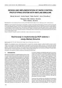
2.0 The MPOD System 2.1.0 Physical Description The MPOD vehicle's primary task is satellite docking. Figure (1) shows the final stages of an underwater docking run. MPOD's octahedral configuration was a compromise between ease of construction and minimization of water drag. A perfect sphere would be the most efficient shape, but would be almost impossible to construct. An octagonal body approaches a sphere, but allows the frame and surface to be constructed from rectangular and triangular components. The vehicle's frame is composed of 1" aluminum box beams, inter-connected with riveted gusset plates and covered by foam and fiberglass panels. Overall dimensions are approximately 2 meters along each of the vehicle axes. MPOD's size was primarily determined by the requirement of an onboard cockpit. The cockpit and pilot entry area comprise the upper and central portion of the vehicle. Pressurization, electronic, and power supply components are contained below and to the sides of the open cockpit. Figure (2) shows a simplified side view of the assembled MPOD with docking probe. With twelve motors driving ducted propellors, the vehicle has the ability to move in the six degrees of freedom associated with three-dimensional free-flight. Since the motors are located in pairs along the vehicle principal axes at a distance of 0.81m from MPOD's center, there are equal thrust levels for all translational directions and equivalent torques about all rotational axes. The motors are driven by MPOD's onboard electronics and power system. Thruster magnitude and direction are determined by either the open-loop commands from a pilot or onboard closed-loop control routines. Sensors for the control system include: 3-axis fluidic rate transducers, pendulum inclinometers, a depth sensor, and the Three-Dimensional Acoustic Positioning System (3DAPS). The sensor information is converted
10
Y/Roll Thruster
Dockin Prob
X
Z/Pitch Thruster
X/Yaw Thruster
Z/Pitch Thruster
Y
Z Scale: 1" = 2.0 MPOD 0
Y/Roll Thruster
2 ft.
Figure 2. MPOD Assembled Side View
X Z
Y
Scale: 1" = 2.0 MPOD 0
3DAPS amplifier
Hand Controlle
Stereo Camera
2.0 Main battery
Main battery
Control 80 cu. ft. air
80 cu. ft air
50 cu. ft air Control Battery
Figure 3. MPOD Top Cutaway View 11
into a state vector estimate by the state calculation computer, hereafter referred to as Lando. Obi-Wan, the control computer, uses the estimated state to calculate appropriate thrust values. A third processor, Yoda, communicates with MPOD hardware and continually looks for new instructions from the operator. See Section 2.3 for computer system details. 2.1.1 Components and their Locations Since MPOD is submerged during operation, all electrical components must be housed in water-tight enclosures. Figures (3), (4a), and (4b) show the locations and relative sizes of MPOD's various boxes and air tanks. Most waterproof housings were constructed from foam and fiberglass (see Reference 6 for construction details). The side main battery boxes each contain three lead-acid battery packs supplying +18V for driving the vehicle's motors. This power is switched on and off by a pneumatically-driven relay, housed inside the cylindrical plexiglass power relay box. Since the instantaneous current draw on this system approached ~100A, all cables and connections were constructed accordingly. The control battery box, located under MPOD's rear air tank, holds three +12V battery packs which run all onboard electronics and computer systems. These batteries also power the cockpit when the vehicle is flown from onboard. Two switches attached to the battery box enable divers to turn electronics on and off from underwater. Current draw from the control batteries during normal operation is ~5.5A. MPOD's control box rests on rails under the pilot seat. Nearly all onboard electronics are contained within this box, with the exception of the solenoids for pneumatic cylinders, the 3DAPS hydrophone amplifier circuit, and the heat-generating motor power transistor block, which is mounted under the pilot seat right arm. Contained within the control box are: 3 computers, 2 microcontroller boards, the pendulum inclinometers, rate sensors, motor control circuitry, and 3 wire-wrapped boards which interface all the hardware I/O and the 3 processors. Note that the 3DAPS receivers and the depth sensor are not shown in Figures (2) (4), but will be discussed in Section 2.2. Two 80 ft3 side tanks supply air for an onboard pilot. They are strapped to MPOD's sides with scuba belts. Connected in parallel, they supply the pilot air through a standard scuba regulator. The 50 ft3 rear air tank provides pressurization for all MPOD systems. A high pressure line runs to the solenoid box for driving the pneumatic cylinders, while a modified second-stage regulator is used to pressurize the vehicle's waterproof boxes.
12
Y X Left Large Air Z
Power
Switch Stereo Camera Translational Hand
Solenoid
ller
Prob Command Small Air
Left Main Battery
Control Battery MPOD Control
Figure 4a. MPOD Disassembled Left Side View
Y
X
Z
Right Large Air
Black & White
3DAPS Amplifier
Regulator /
Rotational Hand Right Main Battery
Figure 4b. MPOD Disassembled Right Side View
13
r
2.1.2 Docking Mechanism As mentioned in previous sections, MPOD's primary task is docking to an underwater satellite mockup. This is accomplished via a removable probe, which latches and then rams its target for secure attachment. Figure (5) shows a close-up view of the probe and its mating drogue.
Jettison Clips
Foam flotation
RAM Cylinders (2)
Attachment bolts (4) 90° apart
Docking (hangs from side of Target pool)
securing nuts
MPOD panel front
Figure 5. Docking Probe and Target During flight, the conical ram fixture remains in a retracted state. The spring-loaded latches are set to capture and engage the circular target opening. Upon MPOD's penetration of the docking fixture, the ram is activated to extend into the target's conical opening. The secure fit of the probe prevents all relative motion between MPOD and the satellite. Both the latches and ram are activated by pneumatic cylinders. The latch cylinder and driving mechanism are contained within the probe, while the ram is activated by the two cylinders visible on the probe's exterior.
14
2.1.3 Pressurization System Air pressurization systems play an important role during vehicle operation. Shown in Figure (6) is a diagram of all MPOD pressure systems. Onboard air for a pilot is required primarily because the cockpit is not large enough for a diver in scuba equipment to fit. The double tank system allows even a heavy breather to fly for an entire test session. The small air tank supplies pressure to all MPOD systems. As a precaution against leakage, all water-tight boxes that do not contain hydrogen-venting batteries are pressurized at 2-3 psi above the outside water pressure. This system has two major advantages: the air leaks out instead of allowing water to leak into the boxes, and the bubbles exuded by a box quickly show the presence and location of leakage before the contents become wet. Air is constantly used, but it has been noted that an onboard operator breathes much faster than MPOD. Depending on the frequency of depth changes, a typical test run in the MIT Pool will use approximately 200 psi of air per hour from the small tank. High pressure lines from the small air tank's first stage reducer activate the vehicle's pneumatic cylinders. These solenoid-activated cylinders operate the main power relay and docking probe. Because pneumatic state changes are activated infrequently during testing, they do not cause a significant drain on MPOD's air supply. 2.1.4 Video A pilot flying MPOD from the surface needs visual information to determine an appropriate command sequence. Currently, two video systems are available for MPOD: a set of color stereo cameras with surface signal decoding circuitry (Reference 23), and one black and white camera with wide-angle lens. Figures (4a) and (4b) show the camera positions on MPOD. Each video system's waterproof housing is mounted inside the vehicle's front panel, with each lens pointing along the +x axis. This location enables the pilot to view the docking probe and the target during approach. Power is sent from the surface to each camera. The video signal runs back through a shielded cable to a surface monitor. Since an operator's ability to fly the vehicle was not the emphasis of this thesis, sophisticated video feedback was unnecessary. The single black and white camera was used for all experiments. It provided a clear view of the target, and enabled the operator to
15
keep a close watch over MPOD's flight progress. The video feedback was also used to determine the exact point at which MPOD engaged the docking target. 2.1.5 Control Box Description and Contents The MPOD control box contains almost all the vehicle's onboard circuitry, and was built to enable relatively simple electronics modifications. Its size was determined by the vehicle frame dimensions, with the box filling the entire space below the pilot seat to within a few centimeters. The control box lid was made of anodized aluminum, serving the dual purposes of covering the box and dissipating the electronics-generated heat. Tension latches and a rubber gasket provided the seal between lid and box. All external connections were made on the box ends, both for sizing and connectability reasons. Small gauge electrical wires were attached with Amphenol™ connectors. The larger (14 AWG) wires exit the box through resin and epoxy-filled threaded brass bulkheads, then terminate with Sure-Seal™ connectors. Fiber optic signals travel through the control box via plastic connectors with waterproofed internal box cables. Since a bulkhead connector significantly lowers the line's light intensity, the 3DAPS fast fiber optic line connects directly with the receiver chip, which has been insulated and mounted on the control box outer surface. MPOD's control box is installed and removed by sliding it along mounting rails out the right side of the vehicle. When not inside MPOD, the box rests on a rollered cart which has the necessary sliding rail system and is the same height from the ground as MPOD's rails. The box lid may be removed and all connectors attached while the control box is not inside the vehicle. This is necessary for efficient debugging of electronics and software. 2.1.6 3DAPS Physical Aspects The 3-Dimensional Acoustic Positioning System (References 2 and 7) was originally built to function independently of MPOD. 3DAPS mechanisms include a series of acoustic emitters, or thumpers, and acoustic receivers, or "hydrophones". Circuitry contained in a metal box at the surface called the sequencer serially fires the thumpers at regular intervals, set by the operator. It also detects when each thumper fires, and sends this information to the underwater receiver. The thumpers are positioned along the corners of a rectangular parallelopiped, and pointed toward the figure's central point. See Figure (7a) for the MIT Alumni Pool thumper locations.
16
12.6 m
Pool Surface
2.94 m
9.87 m 6
2 4
0
7
3 1
5 x MPOD Docking Target
Deep End of Pool
Figure 7a. 3DAPS Thumper
y z
Locations -- MIT Pool
H3
3DAPS Amplifier Box
H2
H0
y
x
z
H1
Figure 7b. 3DAPS Hydroph
17
one Locations on MPOD
Thumpers are constructed of rapid-firing solenoids which move a metal hammer into contact with a plate. This contact produces an acoustic pulse designed to be centered at a frequency of 100 kHz. Also, the solenoid and plate surfaces are connected to wires which produce an electrical pulse upon contact. This pulse is returned to the sequencer, which in turn sends the signal and corresponding thumper number via a 1 Mbaud serial fiber optic line to the 3DAPS receiver system. Because MPOD processors needed real-time access to 3DAPS ranges, the original receiver system was redesigned and built to fit within MPOD's control box. Four Brüel and Kjaer hydrophones (Reference 8) send the received low-level (2-3 mV) acoustic vibration signals to the amplifier circuit. After amplification, the hydrophone signals are sent to the control box, where distances between the four hydrophones and the fired thumper are calculated, and then sent to MPOD's computers for processing. Unfortunately, when the signal was being amplified inside MPOD's control box, RFI noise produced by the twelve motor relays corrupted the acoustic pulse. Thus the hydrophone amplifier circuit was moved to a separate small waterproof box outside the MPOD control box (see Figure (7b) for box location on MPOD). Because noise on the MPOD power and ground lines were also corrupting the low-level 3DAPS signals, a small 6V battery was placed in the 3DAPS box for powering the amplifier circuitry. Since the hydrophones are fragile, they were enclosed in anodized aluminum "cages" to avoid damage from contact with pool walls, divers, and other obstacles. Figure (7b) shows the mounted locations on MPOD of the enclosed hydrophones. The large distance of each hydrophone from the vehicle center enables a better attitude estimate from 3DAPS. Because the long, narrow rods are easily bent, break-away bolts were used for hydrophone attachment to MPOD. 2.2.0 Electronics MPOD's electronic systems may be divided into three categories: (1) hardware control electronics, (2) circuitry for interfacing all the hardware with all the computers, and (3) computers for communication and calculation. Figure (8) shows a block diagram of all MPOD electronic systems and their interconnections. RAM shared between the computers contains common variables and measurements. Intel 8255A multiplexers provide interfacing between all the hardware and computer data buses. A 12-bit A/D converter with multiplexer is used for reading the analog rate and depth sensor outputs, while HCTL-2000's read encoder counts for the pendula. 3DAPS ranges are determined by FORTH-programmed 68HC11 microprocessor
18
boards. RS232 serial ports provide communication with the surface computer and pilot via the fiber optic lines. The following sections describe the MPOD electronic functions. First, a description of control box internal component locations and circuit card functional division is given to provide an overall picture of the actual hardware. Next, each major circuit is examined in detail. 2.2.1 Electronic Components and their Functions The MPOD control box was designed to hold all onboard circuitry and computer systems. Shown in Figure (9) is the internal layout of the components. The three main computers, Yoda, Obi-Wan, and Lando, are mounted next to each other. The disk drive and NOVRAM (non-volatile RAM) cartridges used to store software are mounted near the computers to minimize ribbon cable length. Two 68HC11 microprocessor boards are mounted between the pendula and motor circuitry. They are connected only to the processor interface card, hence, the boards do not have the need to be near any supporting components. Terminal Blocks
(6)
(6)
Relays
Relays
3DAPS Card
Processor Interface Card
MPOD Hardware Interface card
Ampro 286 (Obi-Wan)
+12V, +5V Fuses
Ampro 286 (Lando)
Voltage Regulator #1
Ampro PC (Yoda)
NOVRAM #1
MPOD AXES
(under Pendula mounting)
fiber optics
PWM Circuit card
X
Gyros
Motor Fuses 68HC11 Boards
Voltage Regulator #2
Disk Drive
Terminal Blocks
NOVRAM #2
Pendula
Y Z
Figure 9. Control Box In
ternal Layout
As seen in Figure (9), there are five wire-wrapped circuit cards in MPOD's control box. The three cards opposite the pendula and rate sensors share information and power along a
19
+18V Fuse Terminal Blocks
common edge connector. Together, they perform all the interfacing between the hardware and the processors. The MPOD Hardware Interface Card, or MIC, is connected to Yoda's data bus. Motor magnitudes and directions as well as solenoids are commanded from this card. Also, MIC contains circuitry to process rate sensor, pendula, and depth information. The processed sensor readings are sent to Yoda via 8255's. Appendix A-1 shows the complete circuit diagram for MIC. The Processor Interface Card, or PIC, has two primary functions. First, it connects the three computers (Yoda, Obi-Wan, and Lando) together with dual port RAM. Next, the 68HC11 ports are connected via 8255's to Obi-Wan's data bus for the reading of 3DAPS ranges. Appendix A-2 shows the complete circuit diagram for PIC. The third card opposite the pendula is the 3DAPS Interface Card. The 3DAPS sequencer serial signal decoding circuitry is contained on this card. It also sends power to and receives signals from the 3DAPS hydrophone amplifier circuit (see Appendix A-6 for the amplifier circuit diagram). The 3DAPS Interface Card circuit diagram is shown in Appendix A3. Almost the entire +y section of the control box is devoted to motor circuitry and its wiring connections. The pulse-width modulation circuit is contained on the PWM circuit card, as labelled in Figure (9). Because of the high current requirement of each motor (20 amp maximum), 14-gauge wire was used for all power and motor signal connections. Relays are mounted in two groups of six (see Figure (8)). Each motor is fused, with the fuse mountings along the +y wall of the control box. The final wire-wrapped circuit is used for the conversion of fiber optics light to/from electrical signals. There are five lines: two for Yoda, two for Obi-Wan, and one fast fiber optics line for 3DAPS. The conversion circuit card is mounted next to the onboard disk drive. Appendix A-5 shows the 5-channel fiber optics circuit diagram. 2.2.2 Solenoids Both the docking probe and main power relay are driven by +12V pneumatic solenoids. Figure (10a) shows a single solenoid circuit. The TIP31 transistor is switched by a 1-bit signal from Yoda. The signal then travels from the control box to the solenoid box, where the appropriate device is activated. Upon switching of a solenoid, the pressurized
20
line is vented, then the excess air escapes the solenoid box through a purge valve. Mounted on a six-solenoid manifold, the solenoids switch high pressure from one line to another, depending on the current flow through the electrical lines. Figure (10b) shows the functions of the three solenoids currently used by MPOD. The main power relay is driven by one high pressure hose. Nominally, this line is not pressurized. Upon solenoid activation, the metal relay plate is driven up to meet another matching plate. An electrical connection is then made between the positive leads on the main batteries and the MPOD control box +18V lines. If no pressure is supplied to this line, the relay plate is held away from its mate by springs, and no electrical connection is made. The extension of the docking probe is accomplished by two cylinders driven by the same solenoid pressure lines. The default setting (i.e. with no current passing through the solenoid) is the ram retracted position. Finally, the disengagement of the probe's latches is accomplished by a single pneumatic cylinder. No solenoid current flow results in engaged latches, thus allowing target capture before the line is activated. 2.2.3 Motor Control The motors are activated via a 4-bit magnitude, 1-bit direction command from Yoda, the onboard PC. The actual thrust output by each motor motor is obtained by pulse-width modulation of the driving voltage, determined by the computer's magnitude outputs. Each motor's direction is controlled by a relay. Shown in Figure (11) is a diagram of the circuit for one motor. The 4-bit magnitude command passes through 74HC85 channel A, and is compared to the constantly counting output of an HC163. Since the twelve motors are organized in pairs, only six independent commands are sent from the computer. After passing through the comparator, these six signals are buffered and split into two lines, one for each motor of a pair. Then, the signal passes through a resistor and transistors before reaching the relay. Each motor direction bit was buffered and split into two lines, as was the magnitude signal. The direction bit triggers the relay, which is connected so that the motor is running either forward or backward, for non-zero magnitudes. Because of the high current requirement (maximum of 20A per motor), multiple transistors are necessary for TTL signal amplification. Motor power lines are fused in two separate locations to help prevent circuit components from overloading during the inevitable current spikes. Each 11028 power transistor dissipates a significant amount of heat, so the twelve transistors were waterproofed and mounted on a heat sink outside MPOD's control box. The control box internal layout (see Figure (9)) shows the box location of the motor circuitry. Appendix A-4 shows the complete PWM circuit card diagram.
21
2.2.4 Pendulum Inclinometers A pendulum inclinometer consists of an aluminum weight hung from a rod which is then attached to a freely rotating encoder shaft. One such device aligned with each of the MPOD vehicle's axes. Figure (12a) shows a 3-axis arrangement and possible pendulum positions when the vehicle and inertial axes are aligned. The pendula constantly move to follow the gravity vector, which is assumed to be much greater in magnitude than any feasible vehicle acceleration. y x z
index
HCTL-2000
12-bit value
Quadrature Encoder
a b
g Yoda
Figure 12a. Pendula Layo
ut
Figure 12b.
Encoder Circuit
Pendula positions are determined by BEI Motion Systems quadrature encoders with 12-bit resolution. Figure (12b) shows the basic circuit for one channel. The HCTL-2000 (Reference 9) decodes the a and b pulsing lines, which are 90° out of phase with each other. This phase shift enables the determination of the direction of pendulum motion. Also, an index pulse once per shaft resolution is used to reset the counter in case some counts are missed. At system startup, the HCTL-2000 begins counting from zero. To ensure proper encoder readings after startup, each pendulum must be rotated such that its index pulse is passed. The zero-count for each encoder is then properly initialized.
22
2.2.5 Depth and 3-axis Rate Sensors A 12-bit Analog Devices A/D converter and multiplexer combination (Reference 10) is used to read a pressure sensor and 3-axis rate transducer package. The pressure sensor, Omega PX240 Series (Reference 11), is located at approximately the vehicle's center of mass, and is used to determine MPOD's depth in the water. This sensor receives a +15V input signal and emits an analog voltage between 0 and +7V. The Omega PX240 package is capable of measuring depths up to 20 meters in the water. MIT's Alumni Pool is less than five meters deep. The 3-axis rate transducer package measures MPOD's angular velocity about all three vehicle axes. Driven by +12V input, a fluidic sensor package, Humphrey, Inc., Series RT02, measures rates between ±p/2 rad/sec (Reference 12). Its analog output voltage ranges from 5V to +5V for full scale angular velocities. Calibrations and accuracy of the rate and pressure sensors are described in Chapter 3. Because the sensors were converted by the same A/D, its gain and range were required to be compatible with both sensor outputs. Since the lower bit of depth and lower 3-bits of the rate sensors were noise, the maximum input range of the A/D was set at ±10V. The A/D and multiplexer system is controlled by Yoda. The process of reading an analog sensor value includes the following steps: (1) output desired multiplexer channel, (2) sample and hold the chosen channel, (3) begin A/D conversion process, (4) upon completion of conversion, read the 12-bit converted value. See "yodafuns.c" in Appendix B-1 for the software implementation of the sensor reading. 2.2.6 3DAPS Receiver Electronics and Microprocessor Software 3DAPS, the 3-Dimensional Acoustic Positioning System, consists of both surface and underwater electronics. Figure (13) shows a complete system diagram of 3DAPS. The sequencer drives and receives signals from the eight thumpers, while the receiver system analyzes hydrophone signals and receives contact and thumper identification signals from the sequencer. The sequencer, thumpers, and hydrophones are identical to those in the systems described in References 2 and 7. However, the receiver system was designed and built to function inside MPOD's control box. The previous 3DAPS receiver was primarily hardware-based, with individual counters and gates determining thumper-to-hydrophone ranges. In an attempt to simplify circuitry and facilitate system modifications, most of the prior receiver electronics were replaced by 68HC11 microprocessors (Reference 13) programmed in MAX-FORTH. Upon thumper activation, the sequencer sends a serial signal to MPOD. This signal is decoded into a contact signal bit and 3-
23
bit thumper identification number. Appendix A-3 shows the serial decoding circuit, which is contained on the 3DAPS Interface Card inside MPOD's control box. The contact signal bit triggers a hardware interrupt line on the two 68HC11's. Then, the microprocessors begin counting until they receive a hydrophone pulse on a specified counter interrupt line. Note that each 68HC11 handles two of the four acoustic receivers. Hydrophone signals are amplified by a series of AD521 instrumentation amplifiers, then sent through one-shots to produce a TTL-level pulse. H11L1 Schmitt Trigger optoisolators are used to convert the 3DAPS one-shot signals into MPOD control box signals. This eliminates all electrical connections between the amplifier circuitry and all other MPOD systems. See Appendix A-6 for the complete diagram of the 4-channel hydrophone amplification circuit. Amplifier gains are set such that acoustic interference from other systems is minimized, but all thumpers are received from anywhere in the specified rectangular parallelopiped of flight. 74HC123 pulse lengths are adjusted to prevent post-pulse triggering from acoustic reflections. After the 68HC11's have received all hydrophone signals or counter rollover has occurred, they interrupt Obi-Wan in a declaration of new data. Obi-Wan then reads the current thumper's data, and each 68HC11 awaits the next contact signal. See Appendix B-5 for a complete listing of the software used by the 68HC11's, named Crumb and Cake. The program USMV6811.TXT is used for downloading a program to the 68HC11 for booting and running from the onboard 8Kbyte EPROM (Erasable Programmable ROM). Because a programmed EPROM may not be modified, run-time data is stored on an 8K NOVRAM (Dallas Semiconductor 1225Y non-volatile RAM). A program called INT6811.TXT is stored on the EPROM to perform the 3DAPS counting functions. Each 68HC11 was programmed from RS232 serial lines from an IBM PC. The serial communication program PC-Talk was used on the surface computer for 68HC11 program downloading. 2.2.7 Multiprocessor Interfacing The 68HC11 microprocessors are interfaced to Obi-Wan via 8255A's, arranged in parallel to accommodate Obi-Wan's 16-bit data expansion bus. When data is passed between the two systems, handshaking must occur via two bits on an 8255 line. A block diagram of connections is shown in Figure (14). Appendix A-2 shows the complete interface circuit between Obi-Wan and the 68HC11's. MPOD's three main onboard computers, Yoda, Obi-Wan, and Lando, share common RAM. An Advanced Micro Devices AM2130 Dual Port Ram (DPR) 1 Kbyte device is used for each processor interconnection (Reference 14). Figure (14) also shows the expansion bus connections for the three computers. Yoda and Obi-Wan are connected via one DPR chip,
24
while Obi-Wan and Lando are connected via a second chip. For parameter sharing between Yoda and Lando, Obi-Wan must perform a memory transfer. This was an acceptable solution, due to the fact that Obi-Wan uses all the Yoda and Lando shared data in its own control calculations.
A0-A9
D0-D7
R/W
Busy
Busy
Enable
R/W
D0-D7
A0-A9
A0-A9
D0-D7
R/W
Enable
Crumb -Ports A,B,C,D,E
8255-1
8255-2
8255-3
8255-4
AM2130 - 2
AM2130 - 1 Busy
Enable
Lando -AT Expansion Bus IRQ
A0-A9
D0-D7
R/W
Enable
Busy
Yoda -PC Expansion Bus
D0-D7
Enable-1 D8-D15
Enable-2
R/W & Reset
IRQ
Obi-Wan -AT Expansion Bus A0-A1
Figure 14. Multiple Proc
Cake -Ports A,B,C,D,E
essor Interface Diagram
2.2.8 Fiber Optics Serial communications between MPOD and the surface station are performed through fiber optic cables. This technology allows relatively thin umbilical lines running from the vehicle to the control station. Also, communication problems may be diagnosed by unplugging the cable and examining the light being transmitted through the cables, even while the vehicle is underwater. A bright transmitted light signal indicates proper cable operation, while constant darkness or dull ambient light may suggest a cut in the cable. Hewlett-Packard optical sensing chips, connectors, and cables were chosen (Reference 9). Their products were relatively inexpensive and included bulkhead connectors which could easily be mounted on waterproof boxes. The RS232 serial signals travel at the relatively slow rate of 9600 baud, so the optical transmitter/receiver chips chosen for this system were lowspeed, high sensitivity devices. It has been noticed that small cuts through the cable insulation do not affect this system.
25
The 3DAPS sequencer serial signal is transmitted at 250 Kbaud. Hence, the low-speed devices were not sufficient. The required 3DAPS transmission rate meant using high-speed transmitter/receiver chips which, unfortunately, are not sensitive to low level light. Shown in Figure (15) is a diagram of MPOD and surface serial communication connections. Note that the lines from Yoda and Obi-Wan can both connect with the control station computer's (Luke's) COM1 lines. Since Obi-Wan's serial line is used only for data transmission between test runs, the lines may be switched by the surface operator as needed. Also, because the sequencer does not receive data from the 3DAPS receiver system, only one line is needed. Converter Plastic End Chip Connector 1 2 3 4 1 2 3 4
HFBR -1512 HFBR -2503
Fiber Optic Cable
8 Grey 5 8
5
Blue 5
4 HFBR 3 -2503 21 8
Blue
Yoda
4 HFBR 3 -1512 21 8 5
1 2 3 4 1 2 3 4
HFBR -1512 HFBR -2503
8
Grey Grey
5
Luke -- Control Station
8 Blue 5
Obi-Wan 1 8 2 HFBR 3 -2502 4 5
Grey
Blue
5 HFBR 4 3 -1502 2 1 8
3DAPS Transmitter
3DAPS Receiver
Figure 15. Fiber Optics
Connections
For a complete circuit diagram for all five fiber optics channels, see Appendix A-5. The RS232 signals are converted to fiber optic transmitter levels by a +5V to +12V voltage conversion chip, while received signals are converted back to RS232 levels by a +12V to +5V voltage conversion IC. As depicted in Figure (15), the light conversion chips are shaped to accommodate the snap-in fiber optic end connectors. 2.3.0 Computer Systems MPOD onboard computer processing tasks are divided among three AMPRO single board computers (References 15-18). One processor, Yoda, performs communication tasks,
26
both with the surface operator and all MPOD onboard hardware. A second computer, ObiWan, provides interfacing between the three computers, reads 3DAPS data, computes control outputs, and saves all data. Finally, the third computer in the series, Lando, calculates the MPOD state vector from all the available sensor measurements. The three computers have slightly different components and operate at different clock speeds, but the interfacing and support components are identical for the two 286 boards, and similar for the PC. All the boards run under MS-DOS, and are programmed with Microsoft C, version 5.1. The programs execute within a startup batch file, so that the programs will continuously run without keyboard commands. Each single-board computer may be attached to a standard IBM monitor and AT keyboard (PC keyboard for Yoda). Video signals for each board are provided by a mono/CGA card that attaches directly to each computer's expansion bus. Expansion bus signals are sent through ribbon cables to the MPOD wire-wrapped circuit boards. Because of the CMOS computer components and lengthy ribbon cables required inside MPOD's control box, expansion bus signals are terminated by buffers, except for the low-power dual port RAM. The AMPRO computers are powered by +5V, with a current draw of ~1A, including video card. With maximum dimensions of 6" x 8" x 1" thick, the boards mount easily within MPOD's control box. Because the computers are constructed from CMOS components, the power and heat dissipation requirements are far lower than those for conventional computers.
27
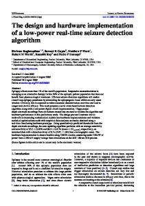
START
Initialize serial port, Y oda variables, Dual Port Ram variables, MPOD hardware, and PiVeCS messages
Has Operator set program escape flag?
Yes
Turn MPOD pneumatics and motors OFF
No
Exit program
Read next PiVeCS message
Activate MPOD Pneumatic changes
Read depth, rate sensors, and encoder values
No
Is Main Power ON? Yes
Output MPOD motor commands
Figure 16. Yoda Software
28
Diagram
2.3.1 Yoda the Communications PC Running at a clock speed of 8MHz, the single-board PC communicates with both the surface pilot and MPOD hardware. Yoda software is stored on the 3 1/2", 720Kbyte disk drive mounted within MPOD's control box. A relatively slow PC was acceptable for communication tasks, due to the minimal number of mathematical computations and speed limitation of RS232 serial ports. Figure (16) shows the logic diagram of Yoda software. Serial communications are performed at a rate of 9600 baud through the fiber optics lines. A software package known as PiVeCS (Pilot-Vehicle Communication System) was written within the Space Systems Laboratory to enable reliable data exchange between robots and their pilots. Operator commands or data streams are transmitted in "Messages", groups of seven bytes or less. The messages begin with an identification header byte and are sent as requested by the user. The total length of the serial data stream may be varied during run-time by turning on or off a particular message transmission. PiVeCS contains a special function called "ShutDown" which turns off all hardware during periods of communications loss between the surface computer and Yoda. This feature is especially useful for the avoidance of a runaway vehicle due to communications problems during flight. In addition to communicating with the surface operator, Yoda performs all the MPOD hardware input/output. Thruster values, calculated by Obi-Wan, are sent by Yoda to the PWM card. The six motor commands corresponding to MPOD's pairs of motors are sent in four bytes: three magnitude bytes (4-bits per motor pair) and one direction byte (1-bit per motor pair). Pneumatic settings requested by the surface operator are output in one byte. Pendulum encoder values are read by Yoda from the HCTL-2000's. Depth and rate transducer data is read by Yoda through the A/D converter. All the data is stored in dual port RAM to enable easy access by Obi-Wan and Lando. A complete listing of all Yoda software is shown in Appendix B-1. PiVeCS source code is presented in Reference 19. 2.3.2 Obi-Wan the Control 286 Board Obi-Wan has four primary functions: (1) saving data on NOVRAM, (2) reading 3DAPS ranges, (3) transferring dual port RAM data between Yoda and Lando, and (4) calculating control outputs from the estimated state vector. Figure (17) shows the complete software diagram for Obi-Wan. The 80286-based computer runs at a clock
29
START
Upon 'BYE' command from surface, exit Kermit
Open data files Run Kermit; set in Server Mode for sending data files to surface computer
Initialize interrupts, Du al Port RAM, Obi-Wan variable s
Has Operator set program escape flag?
Yes
Close data files; exit program
No
Is AUTOEXEC.BAT running?
Save sensor data, if requested Save calculated state, if requested
No
STOP
Save control outputs, if requested Is Closed-loop control flag set?
No
Use hand controller readin gs for motor commands
Yes
Calculate motor commands from control routine
Transfer required Dual Port RAM data between Yoda and Lando
Has 3DAPS interrupt flag been set?
No
Yes
Read thumper ID Handshake Handshake with 68HC11's Output range gates Read first two ranges
Save range data, if requested
Handshake
Handshake
Read other two ranges
Figure 17. Obi-Wan Softw
30
are Diagram
Yes
speed of 12MHz, with an 80C287 CMOS math coprocessor. A 512Kbyte Dallas Semiconductor NOVRAM cartridge (DS1217M/4) connects directly with a 25-pin socket on the AMPRO computer board. Because of the its speed advantages over a disk drive, all data during MPOD runs is stored on Obi-Wan's NOVRAM. After each run's completion, the data is uplinked via Kermit (Reference 20) to Luke, the surface control station computer, for storage on its hard disk drive. Data uplinking is necessary due to the limited memory available on the NOVRAM. 3DAPS range reading is triggered by hardware IRQ9 on Obi-Wan. The interrupt handler routine sets a flag, then when the main driver program sees the flag, the 3DAPS range reading routine is called. First, the thumper ID is read from the sequencer decoding circuit. Then the ranges are read. Handshaking with the two 68HC11's is necessary because of the limited I/O ports available for the 16-bit range values. Each time a 3DAPS interrupt is generated, four ranges are read. To conserve memory and time, range data is only written to the NOVRAM when new values arrive. The third function performed by Obi-Wan is that of dual port RAM data transfer. During closed-loop runs, the only necessary transfers between Yoda and Lando should be the pendula, depth, and rate sensor values. Note that when the surface operator wishes to observe the state, the values must be transferred from the Lando dual port RAM to Yoda's dual port RAM. The primary calculations performed by Obi-Wan involve converting the state estimate into control outputs for the MPOD thrusters. First, Obi-Wan determines the desired state, dependent on which part of a control path MPOD is traversing. Next, the control routine determines MPOD motor commands by multiplying the feed-forward linearized state error values by gains. See Chapter 4 for a detailed description of the control algorithms. The complete listing of Obi-Wan software is shown in Appendix B-2. 2.3.3 Lando the State Calculation 286 Board The sole purpose of Lando is to estimate the current position, attitude, and rates of the MPOD vehicle. Figure (18) shows a logic diagram of the Lando software. Lando is an 80286-based computer running at a clock speed of 16MHz. Like Obi-Wan, Lando has an 80C287 coprocessor and runs from a 512Kbyte NOVRAM cartridge. 3DAPS ranges and the depth sensor are used for position determination. The pendulum encoders and 3DAPS provide attitude measurements, while the rate sensors directly measure vehicle angular velocity about each of the three axes. Unfortunately, no direct measurement of linear velocity is available. An extended Kalman filtering routine with state propagation is used for the estimation process. Chapter 4 describes in detail the implementation of this state calculation algorithm.
31
START
Initialize Interrupts, La ndo variables, Dual Port R AM
Has Program escape flag been set?
Is AUTOEXEC.BAT running?
Yes
No
No
Has new 3DAPS data become available?
STOP Yes
Incorporate new ranges; set flag
No No
Is state being estimated? Yes
No
Is this the first time state has been calculated?
Is there new 3DAPS range data?
Initialize state to center of pool; zero velocity
Yes
Yes
Call filter once for each accurate new range
No Call filter for chosen sensor measurement (ie. pendula, rate, depth) Increment measurement choice for next program l oop
Store new state estimate in Dual Port RAM
Figure 18. Lando Softwar
32
e Diagram
Yes
The filter is called with one measurement at a time. Since 3DAPS ranges are available relatively infrequently, Lando hardware interrupt IRQ9 is activated by Obi-Wan upon receipt of new 3DAPS data. Lando only calls the filter for range measurements when its interrupt line has been triggered and the new ranges are non-zero. Since new pendula, rate, and depth measurements are available as frequently as Lando updates the state for one measurement, Lando cycles through these sensor readings in order, except when interrupted with 3DAPS data. State calculation may be turned "off" and "on", and the state estimate may be re-initialized by the surface operator. Because the filter initially guesses that MPOD is at the center of the 3DAPS thumper parallelopiped, the state calculation routines should be turned "on" when MPOD is near that location.
2.4.0 Surface Control Station For MPOD human factors testing, an attempt was made to make a remote control station as similar as possible to the onboard cockpit. However, the tests performed in this thesis had no human factors component. Therefore, the control station was designed to be easy to assemble and centered around the fastest available IBM-compatible computer. This computer was used for developing all the MPOD onboard programs as well as the control station software. 2.4.1 Pilot Interface and Hardware Description An operator flies MPOD with two hand controllers and the surface computer keyboard. During open loop flight, the left hand controls MPOD translational motion, while the right hand dictates rotational maneuvers. The keyboard is used for controlling MPOD pneumatics, commanding data transmission, and turning on and off the various calculations being performed on MPOD. The operator receives two types of feedback from MPOD: (1) Black and white video from MPOD's camera, and (2) the computer display of PiVeCS, the current switch settings, and uplinked data values. Shown in Figure (19) is a diagram of the surface control station used for the MPOD experiments.
33
Computer Monitor
Fiber Optics Conversion Box MPOD Video Monitor
D:\_ T R
Translational Hand Controller
Rotational Hand Controller 286
Keyboard
Figure 19. Control Stati
on Layout
The computer used for these experiments was a 10MHz 286-clone, hereafter referred to as Luke. Luke has a 40Mbyte hard disk, one 5 1/4" floppy drive, and a 3 1/2" 720K disk drive. An EGA monitor and video card are used. One RS232 serial port is connected to the external fiber optics conversion box for serial transmissions to and from MPOD. A wire-wrapped circuit card, attached to Luke's data bus, connects the hand controllers with the rest of the system. See Appendix A-7 for the card's circuit diagram. The hand controllers used are "bang-bang", meaning they provide on/off signals but no variable magnitude. They use magnets and redundant magnetic field sensors to produce the electrical signals sent to Luke. For a more detailed description, see Reference 6. Note that these hand controllers are waterproof and are also used in MPOD's cockpit during onboard flight control. Figure (20) shows a complete diagram of the surface control station components and their functions. 2.4.2 Software During underwater testing, Luke is used to interface with a surface operator and store data between MPOD runs. Besides communicating with Yoda, Luke displays switch settings and MPOD data on its monitor. The computer constantly looks for operator commands from the keyboard and hand controllers. Figure (21) shows the keyboard layout of commands a
34
pilot may initiate. Figure (22) is a block diagram of the control station software logic. Appendix B-4 shows a complete source code listing of the Luke software. Serial communications with Yoda are performed using the PiVeCS protocols. Messages are passed between Luke and Yoda via COM1, running at a rate of 9600 baud. The operator controls the quantity of serial data transmission through Luke's keyboard. During many debugging situations, it is important for an operator to have the ability to see certain sensor readings, the calculated state, and/or control outputs. However, viewing of MPOD data at the surface significantly slows the loop times of Yoda and Luke. Also, a large data stream delays serial exchange of important parameters, such as hand controller commands. Therefore, during closed-loop control runs, the operator should view only a minimal number of the data parameters. A pilot may use Luke's display to judge the performance of MPOD in real-time. Besides printing the requested vehicle data, the monitor also provides the user with communication and message passing status. In addition to serial port handling, PiVeCS provides a graphic display atop Luke's monitor which enables the pilot to constantly view the status of communications and the current message being transmitted or received.
ESC Luke
State Calculation F1 F2 F3 F4 3daps Pend. Depth Rate
Control Calculation F5 F6 F7 F8 F9 F10 CLon Att. Pos A&P Att. Pos Hold Enter
F11 F12 Dock
= 1 Esc 2 Esc 3 Esc 4 Esc 5 See 6 See 7 See 8 See 9Calc 0Save ALL Yoda Obi Lando Sens. 3daps State Motor State Data Ram Latch
QPos W Pos E Pos RAtt T Att Y Att P-ON I-ON D-ON P-ON I-ON D-ON A P S I DD F P G I HD Gain Gain Gain Gain Gain Gain
POWER
Figure 21. Luke Keyboard
35
Functions
START
Initialize Luke variab les, serial port, PiVeCS messa ges
Does Operator wish to escape from program?
Yes
STOP
No
Parse and dispatch all re PiVeCS messages
ceived
Request data from MPOD as commanded by operator
Read keyboard; send messages to MPOD
Read Hand Controllers Print important inform ation on computer screen for op erator
Figure 22. Luke Software
36
Diagram
3.0 MPOD Dynamics and Physical Parameters Before the implementation of a control system, sensors must be calibrated, relevant vehicle physical parameters determined, and an estimated state vector formed using these values and the available sensor measurements. All equations and calculations were standardized with SI units. This chapter describes the vehicle equations of motion, MPOD physical parameters, and results from the sensor calibration tests. 3.1.0 MPOD Equations of Motion MPOD travels through the water in 3 dimensions with no constraining tether, and has no significant dynamic modes during free-flight. Therefore, MPOD may be treated as a rigid body moving through a viscous fluid. During vehicle motion, hydrodynamic drag significantly affects MPOD's behavior, both in translation and rotation. Because the drag is proportional to the square of velocity, both the translational and rotational equations of motion are nonlinear. MPOD's motors provide the only known linear forces and torques. Unmodelled effects on MPOD include buoyancy offsets from the vehicle's center and water currents produced by MPOD motors, divers, or pool water jets. Because MPOD is balanced each time it enters the water, a buoyancy term in the equations of motion would be a function of balancing success by the divers. MPOD is usually balanced within 0.5 kg of neutral (i.e. one 1-lb. balancing weight), thus buoyancy offsets may be assumed negligible and considered as constant disturbances in the control system. Water currents may also cause significant MPOD motion, but they are unknown in direction and strength. Hence, they cannot be adequately modelled in the equations of motion and were therefore ignored.. 3.1.1 Rigid Body Translation MPOD locomotive force is provided by twelve motors. Linear acceleration is a function of the instantaneous forcing and vehicle linear velocity. The equations of motion along the inertial translational axes are shown in Equations (3.1-1).
37
x = 1 Fx - Cdt x x m y = 1 Fy - Cdt y y m z = 1 F z - Cdt z z m
(3.1-1)
where x,y,z = inertial translation state variables, Cdt = the MPOD translational drag coefficient, Fn = external forcing about the n inertial axis, and m = total apparent vehicle mass. These equations determine the location of the MPOD vehicle's center with respect to the inertial coordinate system. The mass term includes water that is accelerated with the vehicle. The external force, Fn , is produced by MPOD's thrusters. Later in Chapter 3, it is determined that the drag coefficients are the same about each axis. Because the coordinates x, y, and z are in inertial space, each forcing term Fn is a function of both MPOD motor commands and vehicle attitude. The twelve motors arranged in pairs along the vehicle axes are the control actuators. Linear force in body coordinates is provided by two motor pairs aligned with each of the vehicle x, y, and z axes. The direction cosine matrix, C , is used to transform the motor forces along MPOD body coordinates into linear force values along the inertial x, y, and z axes. In Equation (3.1-2), x n,i and x n,b are positions along the inertial and body n-axes, respectively. The Fn,i and Fn,b in Equation (3.1-3) are forces along the inertial and body n-axes, respectively.
x x,i x y,i x z,i
Fx,i Fy,i Fz,i
= C
=
c11 c21 c31
x x,b x y,b x z,b
c12 c22 c32
c11 c21 c31
=
c13 c23 c33
3.1.2 Rigid Body Rotation
38
c12 c22 c32
Fx,b Fy,b Fz,b
c13 c23 c33
x x,b x y,b x z,b
(3.1-2)
(3.1-3)
Vehicle rotation is described in a similar manner. Torques due to motor thrust and hydrodynamic drag dominate the equations of motion. The important difference between the rotation and translation equations is axial cross-coupling due to the moment of inertia matrix, I . The moment of inertia matrix is approximated as diagonal, although there are inevitably small offdiagonal terms which may be considered as "noise" in the equations of motion. From calculations described in Section 3.2 and Appendix C.1, it is shown that the diagonal terms of the I matrix are not equal. The equations of motion for MPOD's 3-axis rigid body rotation are hence given by Equations (3.1-4).
ωx = 1 Tx + I yy - Izz ωyωz - Cdrx ωx ωx I xx ωy = 1 Ty + I zz - I xx ωxωz - Cdry ωy ωy I yy
ωz = 1 Tz + I xx - Iyy ωxωy - Cdrz ωz ωz Izz
(3.1-4)
where Inn = moment of inertia about the n axis, Tn = motor torque about the n axis, Cdrn = rotational coefficient of drag about the n body axis, and ωn = angular velocity about the n body axis. A method of describing attitude is in terms of Euler angles, roll (φ), pitch (θ), and yaw (ψ). Using this method, the final attitude is dependent on the order of command execution. For this thesis, the standard aircraft system was used in which the Euler angles describe the following sequence of maneuvers: (1) yaw, (2), pitch, then (3) roll. If the maneuvers were performed in any other sequence, a different final vehicle attitude would result. Relating changes in the angular velocities to changes in the Euler angles results in a system of coupled nonlinear equations populated with trigonometric terms. A great simplification can be achieved if the attitude is instead expressed in the quaternion system. Expressed in this manner, the evolution of the attitude is still a set of coupled nonlinear ODE's, but involving only arithmetic computations. Reference 21 contains a complete discussion of quaternions and their applications. The four quaternion elements uniquely describe the three-dimensional attitude of an object. They consist of three coordinates describing an axis in 3-D space and a fourth describing a rotation about that axis, as shown in Equation (3.1-5).
q = q0 + q = q0 + q1i + q2j + q3k
39
(3.1-5)
In terms of the Euler angles φ, θ , and ψ, the quaternion vector is defined by: q0 = cos θ cos 1 ψ + φ 2 2 θ 1 q1 = sin cos ψ - φ 2 2 q2 = sin θ sin 1 ψ - φ 2 2 θ 1 q3 = cos sin ψ + φ 2 2
(3.1-6)
The derivatives of the quaternion vector in terms of the vehicle angular velocities, ωn , are: q0 = - 1 ωxq 1 + ωyq2 + ωzq3 2 1 q1 = ω q - ω q + ωzq2 2 x 0 y 3 q2 = 1 ωxq3 + ωyq0 - ωzq1 2 1 q3 = - ωxq2 + ωyq1 + ωzq0 2
(3.1-7)
For all state and most control calculations, the quaternion coordinate system is used. The direction cosine matrix, C , is calculated from the quaternion estimate using the following conversion matrix:
C =
c11 c21 c31
c12 c22 c32
c13 c23 c33
=
1 - 2 q22 + q23
2 q1q2 - q0q3
2 q1q3 + q0q2
2 q1q2 + q0q3
1 - 2 q21 + q23
2 q2q3 - q0q1
2 q1q3 - q0q2
2 q2q3 + q0q1
1 - 2 q21 + q22
(3.1-7)
3.2.0 MPOD Physical Constants 3.2.1 Apparent Mass For an underwater object, the dynamic equations are best modeled by the use of an "apparent" mass, not the actual mass of the object. In Reference 22, it was shown that the apparent mass of a body moving in water is approximately twice the actual mass of the body. This increase in apparent mass is due to induced water velocity around the moving object. Upon construction, MPOD's dry mass was determined to be approximately 1100 lbs, or 500 kg (Reference 30). This value may have changed slightly with the addition of the new
40
control box. However, due to the inability to reassess the MPOD vehicle's mass, the approximate value of 500 kg is assumed still valid. Multiplying the actual vehicle mass by a factor of two, the apparent vehicle mass is: m = 1000 kg
(3.2-1)
3.2.2 Moments of Inertia The moment of inertia matrix, I , is assumed to be diagonal. This simplifies the equations of motion considerably, and is a reasonable approximation given MPOD's symmetric properties. It would further simplify the equations to assume that all diagonal elements of I were equal; however, calculations show that this is not the case. The most accurate way of calculating MPOD's moments of inertia would be to create a finite element model of MPOD, then compute each element's moment of inertia with respect to the vehicle axes. Due to limited time and computer resources, the I values for MPOD were determined using "lumped masses". Major MPOD components were measured, weighed, then modelled as boxes or cylinders. Components used in moment of inertia calculations included: main battery boxes (2), control battery box, 80 ft 3 air tanks (2), 50 ft 3 air tank, control box, motors (12), docking probe, and solid aluminum panels. The remaining MPOD frame mass was modelled as a spherical shell of radius 0.5 m to simplify moment of inertia calculations. Appendix C-1 shows the calculation breakdown. The composite results used in the MPOD equations of motion are:
I =
Ixx 0 0
0 Iyy 0
0 0 I zz
=
80.5 0 0
0 85.9 0
0 0 94.1
(kg -m 2)
(3.2-2)
3.2.3 Maximum Thrust and Torque The twelve MPOD motors each provide an equal amount of thrust. Although the propellers were designed to provide peak thrust at a non-zero velocity, only static tests could completely separate MPOD thrusters from dynamic effects. The maximum output of the thrusters was determined by attaching a spring scale to the MPOD vehicle, then measuring the full-scale force output along each vehicle axis. Each group of four motors produce a maximum thrust of 120 N, or 30 N/motor. The maximum torque was calculated by multiplying the maximum thrust of the four motors by the moment arm from the vehicle center to the MPOD
41
motor location. This moment arm was measured as 0.85 m about each axis. The maximum thrust and torque available for each axis are shown in Equation (3.2-3). Fmax = 120 N Tmax = F max 0.85 m
= 102 N -m
(3.2-3)
3.2.4 Translational Coefficients of Drag MPOD translational coefficients of drag were experimentally determined during terminal velocity tests. Shortly after a constant thrust command was initiated, the vehicle reached a steady state in which the acceleration approached zero. Then, the only terms remaining in translational equations of motion (3.1-1) were the known forcing and drag. It was experimentally determined that the maximum translational velocity along each of MPOD's axes is approximately 0.5 m/sec. Because all axes also have the same maximum thrust value, all translational coefficients of drag are equal. Thus the single translational coefficient of drag, Cdt, is given by Equation (3.2-4). Cdt =
F max = 120 = 480.0 v2max 0.5 2
kg m
(3.2-4)
3.2.5 Rotational Coefficients of Drag MPOD rotational drag coefficients were also evaluated with terminal velocity tests. Analogous with the translation experiments, a constant torque command produced a rotational steady state in which the angular acceleration was zero. Because the tests were done one axis at a time, the cross-coupling velocity term in each equation also vanished. The maximum thrust terminal velocities about the x, y, and z axes are 0.74, 0.62, and 0.62 rad/sec, respectively. The resulting drag coefficients are:
Cdrx =
Tmax = 102 2 ωxmax 0.74
Cdry = Cdrz =
2
Tmax ω2ymax
= 186.3
= 102 0.62
42
2
kg -m 2
= 265.3
kg -m2
(3.2-5)
3.3.0 Sensor Feedback -- Calibration and Accuracy 3.3.1 3-axis Rate Transducer Package The rate sensors, as described in Section 2.2, measure angular velocities between ± p/2 radians/sec. These rates correspond with rate sensor voltage outputs of ±5V and A/D readings ranging from 1024 - 3071, with a theoretical null reading of 2048. However, through all tests, the zero reading of the rate sensors was not consistently 2048, as shown in Appendix C-2. The expected offsets were countered in the state calculation software listed in Appendix B-3. Rate sensor calibration was determined by dividing the maximum A/D reading by the maximum rate sensor reading. Timed terminal velocity tests agreed with the theoretical calibration. The following calibration factor to SI units was used in the MPOD software: (3096 - 2048) Rate Factor = Max A/D count - A/D zero = = 651.9 counts (3.3-1) Maximum Angular Velocity π rad sec 2 The rate sensor noise was within a two-bit count, or 0.006 rad/sec. See Appendix C-2 for static test results showing rate sensor null offset and noise.
3.3.2 Depth Sensor The depth sensor was calibrated by taking MPOD to known water depths and calculating the corresponding sensor readings. The depth sensor has a maximum output of approximately +8V at a depth of 20 or more meters. Because the same 12-bit A/D converter was used for both the angular rate (0-±5V) and depth (0-+8V) measurements, the full-scale readings were set at ±10V. The zero depth value of (2430 ± 2) counts was determined by the surface depth sensor reading. The conversion factor from these experiments is calculated in Equation (3.3-2).
Depth Factor =
Depth A/D Count - Zero depth A/D count = 60.2 counts m Depth in Meters
(3.3-2)
The depth sensor reading was accurate to two bits, or 0.066 m. See Appendix C-2 for the depth sensor standard deviation during static testing with MPOD on various areas of the pool floor.
43
3.3.3 Pendulum Inclinometers The pendulum encoders and HCTL-2000's provide a 12-bit value which ranges from 0 to 4095, as described in Section 2.2. This encoder count corresponds to angles of 0 - 2p radians, thus the calibration factor is given by: Pendula Factor = 12-bit HCTL-2000 Count = 651.9 counts 2π radians per revolution radian
(3.3-3)
Pendulum inaccuracies are produced by dynamic modes of the swinging pendulum weights during MPOD motion. These pendulum modes have a maximum magnitude no greater than four bits, or (0.024 radians), as determined by studying dynamic data. 3.3.4 3DAPS Ranges The range calibration equation depends on the speed of sound in water and the delay between thumper contact and counter initialization. Experimental calibration is the most practical method for precisely determining these parameters. To perform the calibration, MPOD was weighted to the bottom of the pool, then a series of range data was collected. Next, divers manually measured the distances for each thumper-hydrophone combination (8 thumpers x 4 hydrophones). After the experiments were completed, averages and standard deviations of 3DAPSdetermined counts for each thumper-hydrophone combination at each static location were determined. The average ranges were plotted against the measured ranges. Next, a linear curve fit was performed to determine the offset and range factor for the conversion from counts to meters. Equation (3.3-4) shows the calibration equation used in the state calculation software. Figure (23) shows the composite range calibration plot for three different MPOD locations. The standard deviation of the ranges averaged 42.7 counts, or 0.032 meters. Range (m)
= 1.011 + 0.000748 Range (counts )
44
(3.3-4)
20000
Range(counts)
y = - 1344.7 + 1336.2x R^2 = 0.999
10000
0 2
4
6
8
10
12
14
Range(m)
Figure 23. Static Range Calibration Plot
45
4.0 The Control System The goal for the current MPOD multiprocessor system is automated docking from any initial starting point. A fully operational control system would include: 3-axis position hold, 3axis attitude hold, and inertial trajectory following. Any combination position and attitude maneuver should be possible. The controller should be sufficiently robust to counter slight MPOD buoyancy offsets and water currents, which may be considered disturbances by the control system. This thesis does not present a thoroughly tested and proven controller. However, algorithms and MATLAB linearized control results are presented for possible future implementation. With gain adjustments, it is expected that the current algorithms are capable of performing many of the control system goals, from station-keeping to automated flight. Before the implementation of a control system, sensor measurements must be used to estimate vehicle position, attitude, and velocity. This chapter first describes the state estimation equations and their implementation. Next, a position and attitude hold control system is developed by linearizing the equations of motion about a set point. Finally, the full nonlinear dynamic model is incorporated into a feed-forward linearization control scheme for large position and attitude maneuvers.
4.1.0 State Calculation 4.1.1 State Vector Elements and their Derivatives In order to fully examine the dynamic properties, MPOD's translational and rotational position and velocity must be estimated. Also, the unpredictable null offset in the rate sensor readings, bn , must be estimated for each measurement sequence. Equation (4.1-1) shows the components of the 16-dimensional estimated state vector. y = y1 y2 = x y z
y16
T
q0 q1 q2 q3 vx vy vz
ω x ω y ω z bx by bz T
(4.1-1)
A new estimate of this state vector is determined each time the filter incorporates a new measurement. Because the equations of motion are integrated during the state estimation
46
process, the derivatives of all state vector elements must be calculated. These equations were described in Chapter 3. Equation (4.1-2) shows the complete state derivative vector. v x q0
1 -q T ω 2
q
q0 ω + q x ω
y =
=
(4.1-2) 1 F- c 2 dt v sgn v m
v ω
I -1 T - c dr ω2 sgn ω - ω x I ω
b 0
4.1.2 Extended Kalman Filter Equations Reference 23 describes in detail the derivation and implementation of the extended Kalman filter equations for MPOD. Equations (4.1-3) show the extended Kalman filter equations used in the MPOD state calculation software.
P
+
T
= I - k i hi
+
-
y = y + k i gi - zi
P
-
(4.1-3)
where P = error covariance matrix gi = ith expected measurement
zi = ith actual measurement y = State vector estimate hi =
Žgi
= Sensitivity of ith measurement to variations in
Žy ki = 1 P - hi = Measurement gain a
47
y
T
where a = σ2 + h i P - hi and σ2 = variance of sensor i output +/- superscripts = quantities after/before measurement incorporation These equations are updated upon receipt of each new measurement, zi. MPOD filter software is listed in Appendix B.3, "filter.c". The filter update rate during MPOD runs is approximately 50 measurements per second. 4.1.3 Measurement Incorporation and State Propagation Each of the measurements gives information about a combination of state vector elements. To predict MPOD's 39 sensor measurements, correlation between these measurements and state vector elements must be determined. Equations (4.1-4) show the relationship between the thirty-two 3DAPS range readings and state vector elements.
gij = d ij
T
d ij = r ij
dij = x + C l i - tj
2
(4.1-4)
where rij = range value from hydrophone i to thumper j, dij = range vector from hydrophone i to thumper j, C = direction cosine matrix defined in Chapter 3, l i = hydrophone i position vector with respect to MPOD body coordinates, and t j = thumper j position vector with respect to inertial coordinates. Note that l i and t j are constant vectors. The pendula produce the most complex combinations of state vector measurements. Because they measure only the gravity vector, the inertial yaw reading cannot be determined with pendulum feedback. The following equations relate the three pendulum measurements to the inertial space. Note the loss of yaw angle sign information due to taking the cosine of pendulum angles. To restore the yaw angle sign information, the pitch angle sign is incorporated into the measurement. Equation (4.1-5) shows the state parameters relating to the pendulum measurements.
48
gφ =
c33 = cos(φ) , c32 2 + c33 2 gψ =
c33 = cos(θ), c31 2 + c33 2
gθ =
- sgn gθ c31 c31 2 + c32 2
= cos(ψ)
(4.1-5)
where the cij are elements of the direction cosine matrix. The three-axis rate sensors proportionally affect only the angular velocity (ω) elements of the state vector, while the depth sensor provides a direct inertial z - coordinate measurement. Equations (4.1-6) show the correlation between measurements and the corresponding state vector elements.
gω = ω + b =
ωx, meas ωy, meas , ωz, meas
gz = z = (depth)
(4.1-6)
In order to determine, at each iteration, how to adjust the current state vector estimate, it is necessary to evaluate the effect on the expected measurements of first order perturbations in the estimated state. For this reason, it is necessary to calculate all measurement derivatives with Žg respect to the estimated state vector elements, Žy . Equation (4.1-7) shows the elements of this measurement derivative matrix. Because of the complexity of the 624 results, they will not be presented in this thesis. Reference 23 shows the complete set of derivatives used in the MPOD filter calculations.
Žg Žy
Žg r Žx
Žg r Žq
Žg r Žg r Žg r Žv Žω Žb
Žg p
Žg p
Žg p Žg p Žg p
Žx
Žq
Žv
Žg z Žx
Žg z Žq
Žg z Žg z Žg z Žv Žω Žb
Žg ω Žx
Žg ω Žq
Žg ω Žg ω Žg ω Žv Žω Žb
=
49
Žω
Žb
(4.1-7)
where g r = range measurement vector, g p = pendula measurement vector, g z = depth sensor measurement vector, and g ω = rate sensor measurements. In addition to incorporating measurements during the state estimation process, MPOD equations of motion must also be integrated. Estimates of vehicle positions, velocities, and applied forces are used to calculate vehicle acceleration components. See Equations (4.1-2) for the state vector derivative components, yi. After calculating all the state vector derivatives, the yi equations are integrated using a second-order Runge-Kutta algorithm. The integration procedure uses an intermediate estimate y t + ∆t / 2 between the times t and (t + ∆t). See Reference 23 for details. Appendix B.3 shows the MPOD state propagation software in "pstate.c". 4.2.0 Position and Attitude Hold 4.2.1 Linearized Equations of Motion Because more theory is available for linear control systems analysis, an attempt was made to linearize MPOD equations of motion whenever possible. For small attitude or position changes, the second order terms may be ignored, thus producing linear equations about which a linear PID control system may be implemented. MPOD maneuvers may be considered small during station-keeping, or set point regulation. If the desired position is given by x n,0 and the current position is x n, then position perturbations from the nominal value are given by x n,0 - x n . The linear velocity is given by δv . For attitude, small perturbations about a set point may easily be represented by the use of Euler angles instead of quaternions. The conversion from quaternions to the Euler angles is given by: θ = -arcsin c13 = -arcsin 2* q1q3 - q2q0 ψ = - arctan2
c23 , c33 = - arctan2 2 q2q3 + q0q1 , 1 - 2 q21 + q22 cos θ cos θ cos θ cos θ
φ = - arctan2
c12 , c11 = - arctan2 2 q1q2 + q3q0 , 1 - 2 q22 + q23 cos θ cos θ cos θ cos θ
(4.2-1)
Under the small perturbation assumption, second order drag and cross-coupled inertia terms in the equations of motion may be neglected, such that both the translational and rotational
50
equations described in Chapter 3 become double integrators. The state-space form of linear equations of motion is given by:
x = A x + B u
(4.2-2)
The MPOD linearized equations of motion are:
δx n δx n
δωn δΦn
= 0 1 0 0
= 0 1 0 0
x n,0 - x n δx n
Φn,0 - Φn δωn
+
0
Fn
(4.2-3a)
Tn
(4.2-3b)
1 m
+
0 1 Inn
where Equations (4.2-3a) represent translation and (4.2-3b) rotations. For convenience, the matrices in (4.2-3a) will be denoted by Ax and B x while the matrices in (4.2-3b) will be AΦ and B Φ . 4.2.2 Proportional-Integral-Derivative (PID) Control Structure For a double integrator system, the actuator outputs are determined by multiplying position and velocity estimate errors with "proportional" and "derivative" controller gains, respectively. To prevent steady-state errors, the position is integrated with respect to time, then multiplied by a gain to provide the "integral" term of the controller. Because each position loop and each attitude loop is completely independent, the PID controller was designed for a single-axis system, then the individual gains were applied to all axes of the multivariable system. A complete position control diagram is shown in Figure (24a). For position regulation, the set point, x 0, is initialized upon control system activation. Errors from the nominal position value are fed into the PID system. Note that the control system only receives the estimated state determined from sensor measurements. The detailed PID position diagram is shown in Figure (24b). The proportional gain corrects the current position error, while the derivative gain is used to damp non-zero velocities. The integral gain is used to keep steady-state errors in line. With a nonzero position error, the
51
integral terms grow with each time step, inducing MPOD to return to its set point position. For software implementation, a maximum limit was placed on the integral feedback term, due to the possibility of an unstable system. During attitude regulation, MPOD must point in a constant direction with respect to the inertial coordinate system. Figure (25a) shows the complete attitude system diagram. As with position, the initial attitude upon control system initiation is used as Φ0, the set point. Then errors between the estimated attitude, Φ, and set point attitude are fed to the PID controller, which is depicted by Figure (25b). The structure of the open-loop MPOD system is shown in Equations (4.2-4), where T(s) is the PID open loop transfer function, where the Kn are gains to be determined. K + KP s + KD s 2 KI + K P + K ds = I s s3
T(s) = 1 s2
(4.2-4)
Note that for certain gains, the system may contain unstable right half-plane poles. The PID closed loop poles and zeros of a double integrator dynamic system are given by the transfer function, C(s), shown in Equation (4.2-5). The next section describes one method by which control system gains may be determined. The results are only an example of many possible methods for gain calculation, and should be considered accordingly.
C(s) =
T(s) 1 + T(s)
=
s2 K D + s K P + K I s 3 + s2 K D + s K P + K I
(4.2-5)
4.2.3 LQ-Servo with Integrator Results The Linear Quadratic Servo problem (Reference 24) provides an optimal stable solution for the gains of a linear PID control problem. The solution relies on the minimization of a cost function, J, which is described in Equation (4.2- 6). ∞
y T Q y + u T R u dt
J=
(4.2- 6)
0
The matrices Q and R are to a certain extent arbitrary. For simplicity, the [Q] matrix was chosen to be the identity matrix. Because MPOD has only one forcing input per equation, [R] was one-dimensional, hereafter labelled ρ.
52
To incorporate the integrator into the state-space equations, the state vector is augmented. Equations (4.2- 7a) and (4.2- 7b) show the position and attitude augmented state equations for control gain analysis. Note the addition of two new variables: w, the position integral variable, and a, the attitude integral variable.
w δx δx
a δω δω
0
w
0 1 0 = 0 0 1 0 0 0
x n,0 - x n
+
δx
Φn,0 - Φn
Fn
(4.2- 7a)
Tn
(4.2- 7b)
1 m 0
a
0 1 0 = 0 0 1 0 0 0
0
+
δω
0 1 Inn
For a closed loop LQ-Servo system, the forcing is determined by the estimated state feedback and desired set point. The control and closed-loop state-space equations are: u = - K x - x set x =
A - B K
x + K x set
(4.2- 8)
Note that x set in the above equations replaces the x0 and Φ0 elements of x in Equations (4.27). The LQ-Servo gain matrix is calculated with the Control Algebraic Ricatti Equation (CARE). Equation (4.2- 9a) shows the CARE. The solution of CARE, L , is used for determination of the control system gain matrix, K = KI KP KD . Equations (4.2-9b) shows solution for K . - L A - A T L - Q + L B R -1 B K = R -1 B
T
L
53
T
L = 0.
(4.2- 9a) (4.2- 9b)
Appendix E.1 shows the position LQ-servo results. The Macintosh MATLAB program was used for all control system analysis. For the "cheap" control problem with ρ = 0.0001, optimal position gains were determined to be: Kx =
K I,x K P,x K D,x =
100.0
447.5
951.3
N m
(4.2- 10)
The limiting factor in control system gains was the maximum available actuator output. The value of ρ was chosen such that the thrusters would saturate when MPOD was a distance of 0.3 m from the desired set point. The system gains were tested by simulations of the linearized equations with an initial position offset of 0.3 m from the desired set point, then with a constant disturbance of magnitude 10 N, to represent water currents. Resulting plots are shown in Appendix E.1. The response time of the system, due to control gains limited by available control authority, was approximately 10 seconds. Overshoot was 50%. This value is quite large, indicating the need to introduce more system damping. Appendix E.2 shows the attitude LQ-servo results. Note that this sample single-axis LQ-Servo used the average of the three moment of inertia values for gain determination. For ρ = 0.0001, optimal rotation set point gains were determined to be:
KΦ = KI,Φ KP,Φ KD,Φ =
100.0
242.0
242.8
N-m
(4.2- 11)
As with position, the value of ρ, and hence the system gains, were limited by thruster power. Gains were chosen such that the thrusters would saturate at 0.5 radians from the set point. The system gains were tested with an initial attitude offset of 0.5 radians, then with a constant disturbance of magnitude 10 N-m which represents a buoyancy offset. Note that this disturbance value is much larger than would be expected in real applications. Plots of the tests are shown in Appendix E.2. The response time was approximately 5 seconds, half that of the position response. The maximum overshoot is 25%. As with the position response, this high value should be countered with more system damping. 4.3.0 Automated Maneuvers 4.3.1 Feed-Forward Linearization Structure When performing large magnitude position and attitude maneuvers, velocities are not small, so the equations of motion may not be linearized as in Section 4.2. A control scheme
54
known as feed-forward linearization has been developed to enable nonlinear dynamic systems to be controlled as if they were linear. Reference 25 describes the rationalization behind this linearization procedure. The main purpose of feed-forward linearization is the cancellation of nonlinear dynamics by feeding forward these terms through the control output. For position, the only nonlinear term in the equations of motion is drag, which is proportional to the square of velocity. Because the state estimator provides a value for the linear velocity, the drag may be estimated. By subtracting the drag term from the control force, the net drag force entering the MPOD plant is zero. Thus the system behaves as if drag were not present. Figure (26a) shows the position feed-forward control diagram. Note the addition of drag to the plant dynamics. The control block of Figure (26a) is expanded in Figure (26b). Except for gain values, the PID portion of the controller is identical to that described in Section 4.2 for regulation about a set point. However, a new feedback path is introduced. Equation (4.3-1) describes the control forcing output, F n, given estimated states values of xn , xn and desired state values of xn,d , xn,d .
Fn = GP,x xn,d - xn
+ GI,x
xn,d t - xn t dt + GD,x xn,d - xn + Cdt xn xn
(4.3-1)
For attitude, drag is only one of two nonlinear terms in the equations of motion. The other term arises from cross-coupling produced by the term ω x I ω. As with drag, this nonlinear inertia term may be cancelled by the actuator torque, Tn. Figure (27a) shows the complete system diagram for large attitude maneuvers. The plant dynamics are affected by both the drag and cross-coupled inertia terms. Because the attitude is expressed in inertial coordinates while the angular velocity and acceleration are in body coordinates, the nonlinear kinematic inversion depicted in Figure (27a) must be performed on the desired and estimated vehicle attitude elements. The attitude controller then receives the angular velocity discrepancy from a desired value, so that a proportional-derivative control system may be implemented with respect to each of the body axes. Figure (27b) shows the detailed control scheme with the feed-forward nonlinear terms. Hydrodynamic drag and inertia cross-coupling are fed through the control system to cancel the nonlinear dynamics. Equation (4.3-2) shows the elements of the control torque, Tn, with angular velocity estimate ωn and desired angular velocity ωn,d.
Tn = GP,Φ
ωn,d t - ωn t dt + G D,Φ ωn,d - ωn + Cdrn ωn ωn - ω x I ω n
55
(4.3-2)
4.3.2 Feed-Forward System Gains The PID feed-forward system gains may be determined as for any linear PID system. The only limiting factor is the control authority used by the feed-forward terms. The maximum expected force required to cancel the translational drag term would occur when MPOD is moving at terminal velocity, x = 0.5 m/sec. The required force to completely cancel this term is equal to the MPOD maximum thrust value of 120 N, by the definition of terminal velocity in Chapter 3. This means that the feed-forward drag term will always have the capability to cancel nonlinear plant dynamics, but may also limit the PID control authority. For attitude, the maximum required torque to completely cancel rotational drag is also equal to the terminal angular velocity about each axis. The same thruster saturation condition is true for attitude as was true for position. Finally, the nonlinear inertia term is always small in magnitude, due to only slight differences in axis moments of inertia. Therefore, there is no chance that the cross-coupled inertia term will alone cause thruster saturation. The feed-forward linearization scheme is easy to implement, while still accounting for nonlinear terms in the equations. This system should be considered for the MPOD control system used for large attitude maneuvers.
56
5.0 Experiments and Test Results MPOD underwater tests were conducted at the MIT Alumni Pool. Because the pool was used for swimming during normal hours, tests were held every 2-3 weeks on Saturday nights and the following Sunday mornings. The main disadvantage to such a schedule was the infrequency of testing and inability to debug many problems in time for the rest of the test session. For example, 3DAPS on MPOD could only be tested while both were completely submerged, so that with each modification, a long wait followed during which there could be little debugging. MPOD and 3DAPS would then be placed back in the pool, only to find that the supposed "solution" to the problem had not actually been effective. Many MPOD pool tests were used for debugging 3DAPS in this manner, primarily because of the inability to find errors between test sessions. All pool test data presented in this thesis was gathered during the weekend of April 2122, 1990. Static data from previous pool tests was valid; however, the 3DAPS calibration offset had changed with the conversion from NOVRAM to EPROMs in the microcontroller boards. This range offset will be the same so long as the 68HC11 software is not modified. The calibration parameters in Chapter 3 were valid for all pool test data presented in this thesis. The experiments were conducted and analyzed in the following order. First, static tests were performed in which MPOD's location could be determined empirically without relying on the data. Second, to distinguish translation maneuvers from attitude movements, a balanced MPOD was flown in an upright attitude between two fixed points. Finally, attitude maneuvers were included in free flight testing. Before studying the state estimator's performance in underwater tests, relatively ideal surface experiments were performed in simulation. In addition to providing unlimited time for data collection, the simulator provided its own state calculations, with which the state estimations were quantitatively compared. This chapter presents a description of the simulation algorithms and test results for the study of state estimator performance. Following simulation results, state calculation data from underwater MPOD tests is presented with a qualitative performance analysis.
5.1.0 MPOD Simulation
57
Two simulation programs were written to run on the MPOD computers. They were performed on Obi-Wan because it was a 286 processor with math coprocessor, had access to all dual port RAM, and had the least responsibility during state calculation tests. 5.1.1 Dynamic Simulation Description The simulation software was implemented on MPOD because of the speed of the available parallel processing and the ability to debug most of the software in its flight configuration. The first of the two simulations was written to enable testing of both the state calculation and future control systems. The operator may choose any initial position and attitude, assuming a zero initial velocity. For dynamic tests, the control station hand controllers may then be used to "fly" the simulator as the vehicle would be flown. Both simulated and estimated data were viewed on the screen, with the option of data saving on Obi-Wan's NOVRAM. The dynamic simulation software is shown in Appendix D.1. The hand controller commands are converted to thrust and torque values which are used in the simulation equations, then sent to the filter. For integration of the equations of motion, the dynamic simulator uses a fourth order Runge-Kutta algorithm. Reference 26 describes the software used in the MPOD simulation. After the simulator calculates the expected MPOD states, sensor measurements are calculated. Because the real sensors contained a known amount of uncertainty, the simulated sensor measurements were each corrupted by random noise proportional to twice the corresponding actual expected sensor noise. This value was chosen to account for unexpected sensor behavior, and examine the filter response when suboptimal conditions were present. Because the simulation and filter software were running on different computers, the loop times were slightly different. Therefore, the simulation and filter time steps used in the equation of motion integrations did not precisely match. This could have been advantageous for analysis purposes, due to the fact that the state estimation loop does not exactly integrate at real-time. The simulation software contained the same dynamic parameters as the filter software. Because the actual MPOD parameters most likely do not agree with the numerical estimates, MPOD dynamics could later be modified in the simulator in order to observe the resultant estimated state discrepancies. It is expected that at least the linear velocity estimate will not match nearly so well, due to the fact that no sensor feedback is available. Another useful addition to the simulator would be disturbance modelling. By applying disturbances to the simulator equations of motion only, the filter would be forced to rely on the sensor measurements for disturbance rejection. In this manner, MPOD's ability to calculate its state despite water currents or buoyancy offsets may be examined.
58
5.1.2 Simulation Static Tests Although the filter should ideally be started when inertial and MPOD body axes are aligned, this is not always feasible. When starting near the filter initialization point, the state estimate consistently converges to the proper value. However, the filter may not converge to the actual state if MPOD is sufficiently far from the initial estimate. The simulator was used to test the filter's ability to converge to a new state, given the initial state estimate of the pool center, or x=0, y=0, z=2 m, with inertial and body axes aligned. Figures (28) and (29) show the position results for different static locations. The first figure shows estimates derived from a low initial covariance (P = 0.2 m), which indicates to the filter that the state estimate is "close" to the actual state. Figure (29) shows the state estimates when a high initial covariance (P = 3.0 m) is passed to the filter, indicating a high level of uncertainty in the current state estimate. Three possible static positions are shown. With all the runs, the large initial covariance produces a large overshoot in state estimate. However, the low initial covariance runs require much more time to stabilize to the final value; for example, in the second run, with x=-3m, y=0m, z=3m, the low initial covariance barely converges after 35 seconds, while the high initial covariance run for the same static point overshot by up to a meter, but settles to the correct value within 6 seconds. Except for the z=1m coordinate in the third static position run, all the static positions shown in these figure settle to their correct steady-state values. In both the high and low initial covariance runs, the z=1m location in the third run settles to ~1.2 m. Perhaps with more testing and further covariance parameter tests, the position behavior
59
Figure 28. Static Simulation Position Plots with Low Initial Covariance
Static Simulation Positions (x=3m, y=3m, z=3m) 3.5 3 2.5 2 1.5 1
x (m) y (m)
0.5
z (m)
0 -0.5 0
1
2
3
4
time (sec)
5
6
Static Simulation Positions (x=-3m, y=0m, z=3m) 6
x (m)
4
y (m) z (m)
2 0 -2 -4 0
5
10
15
time (sec)
20
25
30
35
Static Simulation Positions (x=2m, y=-4m, z=1m) 3 2 1 0 -1
x (m)
-2
y (m) z (m)
-3 -4 0
5
10
time (sec)
60
15
20
25
Figure 29. Static Simulation Position Plots with High Initial Covariance
Static Simulation Positions (x=3m, y=3m, z=3m) 6 5 4 3 2
x (m) y (m) z (m)
1 0 -1 0
2
4
6
8
10
12
time (sec)
Static Simulation Positions (x=-3m, y=0m, z=3m) 4 3 2
x (m) y (m)
1
z (m)
0 -1 -2 -3 -4 0
2
4
6
8
time (sec)
10
12
Static Simulation Positions (x=2m, y=-4m, z=1m) 8 x (m) y (m)
6
z (m)
4 2 0 -2 -4 -6 0
2
4
6
time (sec)
61
8
10
12
14
may be assessed and better predicted. However, the current recommendation remains to start the filter near the pool center, which is the defined zero point in the software. Figures (30) and (31) show the static test results for attitude convergence to a known value. Three distinct convergence cases were shown in static tests, one with the low initial covariance value of P=0.02, and the other with the high initial covariance value of 1.0. For a 180° pitch angle, the initially high covariance system converges to the proper attitude within 6 seconds, while the initially low covariance run shows the beginnings of convergence after 30 seconds of testing. The worst steady-state error in the static simulations was observed during the second test, representing a -90° yaw attitude. This discrepancy may partially be due to the fact that pendula do not assist in the state estimation, while in the other two runs, the pendula do provide information about the altered vehicle state. The quaternion elements q1 and q3 converge to the proper values within 5 seconds, however, q0 is low by approximately 0.1 in both runs, while q2 is unexpectedly nonzero, at a steady-state magnitude of -0.3. A long-duration run of more than a minute was conducted which confirmed that the quaternion elements were indeed experiencing steady-state errors, not just slow transient responses. No solution to this problem has yet been found, although it is suggested that initial covariance and state variance parameters be varied, with the hope of finding some relation between convergence and filter parameters. The final attitude test shown in Figures (30) and (31) is a static 90° roll angle. Yet a third convergence case was observed. The low initial covariance run produced quaternion elements to within 0.1 of the desired value within 4 seconds, but the high initial covariance run never converged. Note the interesting sinusoidal behavior of the zero quaternion elements. As previously stated, the best guarantee of a filter with no steady-state error is to start the state calculations with the vehicle near the initialization point of the filter software. From the static tests, it appears that position converges to the proper steady-state value more easily than attitude, and is not as sensitive to the choice of initial covariance. However, further tests need to be performed to quantify the affects of filter parameters on static state estimate convergence. 5.1.3 Simulation Dynamic Tests By using the simulator to generate dynamic MPOD data, the "actual" vehicle state is always known. Performance of the state estimator may then be determined by comparing its estimate with the actual state as a function of time. Figure (32) shows the positions
62
Figure 30. Static Simulation Attitude Plots with Low Initial Covariance
Static Simulation Attitudes (180° Pitch) 1
0.5
0 q0 q1
-0.5
q2 q3
-1 0
5
10
15
20
time (sec)
25
30
Static Simulation Attitudes (-90° Yaw) 1
0.5 q0
0
q1 q2 q3
-0.5
-1 0
5
10
time (sec)
15
20
25
Static Simulation Attitudes (90° Roll) 1.2 1 0.8 0.6
q0
0.4
q1 q2
0.2
q3
0 -0.2 -0.4 0
2
4
time (sec)
63
6
8
10
Figure 31. Static Simulation Attitude Plots with High Initial Covariance
Static Simulation Attitudes (180° Pitch) 1.5 q0
1
q1 q2
0.5
q3
0 -0.5 -1 0
2
4
6
8
time (sec)
10
12
Static Simulation Attitudes (-90° Yaw) 1.5
q0 q1 q2
1
q3
0.5 0 -0.5 -1 0
2
4
6
time (sec)
8
10
12
14
Static Simulation Attitudes (90° Roll) 1.5 q0 q1
1
q2 q3
0.5 0 -0.5 -1 0
5
time (sec)
64
10
15
during a typical dynamic state calculation run. The x and y estimated position curves match the actual state curves in both shape and magnitude. However, the estimated z value does not agree, by up to a ~1.7 m discrepancy. As expected, the estimated linear velocity curves shown in Figure (33) are not quite so accurate as the position plots. The estimated z-velocity matches the actual value up to approximately 20 seconds into the run, at which point it appears to mirror the actual value. This seems to indicate that the z-thrust is being used in an inverse sense by the estimator. Currently, the source of this error is unknown. Figures (34) and (35) show the quaternion elements of the state vector. The first quaternion shows two distinct spikes at times of approximately 38 and 44 seconds into the run. It is suspected that these are associated with the "state variance" being added to the covariance during each filter loop. Although its magnitude is only 0.0001 for these calculations, the state variance boosts the covariance values by 0.005 every second. This may be significant in attitude calculations. Except for the initial startup transient and two spikes of maximum amplitude 0.4, the quaternion estimates q0, q1, and q2 match the actual state to within 0.006 of their actual values, while q3 has a maximum error of magnitude 0.12. By studying Figure (36), the q3 discrepancy may at least partially be explained by the yaw velocity error. This error is due to the simulated null offset of the yaw rate sensor. Starting at a simulated initial offset of 0.15 rad/sec from the filter expected offset value, the estimated yaw velocity underwent transient behavior to account for the unexpected rate sensor null offset. Note that the roll and pitch angular velocities shown in Figure (36) are accurate to within 0.05 rad/sec for the entire simulation run. Although no definite conclusions may be drawn from the dynamic simulation results performed to date, it seems that the state estimator is performing its job reasonably well. Two positions and three quaternion elements were acceptably accurate, with one quaternion possibly corrupted by rate sensor null offset and one position corrupted from an undetermined source. Hopefully with insight gained by more covariance and state variance analysis, all elements of the state vector will consistently agree with dynamic simulation results. 5.1.4 Real-time Simulation using Pool Test Data The state calculation software had not been thoroughly debugged before the MPOD pool test in which the data was collected. Therefore, a simulation was developed in which the pool test data could be fed into the state estimation software exactly as it would have
65
Figure 32. State Estimator Position Tracking
Dynamic Simulation -- x (m) 1 0
x (m) x (est)
-1 -2 -3 -4 -5 -6 0
10
20
30
40
50
time (sec)
Dynamic Simulation -- y (m) 0.5 y (m)
0
y (est)
-0.5 -1 -1.5 -2 -2.5 -3 0
10
20
time (sec)
30
40
50
Dynamic Simulation -- z (m) 7 6 5 4 3 2 z (m)
1
z (est)
0 -1 0
10
20
time (sec)
66
30
40
50
Figure 33. State Estimator Linear Velocity Tracking
Dynamic Simulation -- x-velocity (m/sec) 0.2 vx vx (est)
0.1 0 -0.1 -0.2 -0.3 -0.4 0
10
20
30
40
50
time (sec)
Dynamic Simulation -- y-velocity 0.1 0 -0.1 -0.2 -0.3
vy vy (est)
-0.4 0
10
20
time (sec)
30
40
50
Dynamic Simulation -- z-velocity 0.6
vz vz (est)
0.4 0.2 0 -0.2 -0.4 0
10
20
time (sec)
67
30
40
50
Figure 34. State Estimator Attitude Tracking (q0 & q1)
Dynamic Simulation -- q0 1.2 1
q0 q0 (est)
0.8 0.6 0.4 0.2 0 -0.2 0
10
20
30
time (sec)
40
50
Dynamic Simulation -- q1 0.2 q1 q1 (est)
0.1 0 -0.1 -0.2 -0.3 -0.4 -0.5 -0.6 0
10
20
30
time (sec)
68
40
50
Figure 35. State Estimator Attitude Tracking (q2 & q3)
Dynamic Simulation -- q2 1 0.8 0.6 0.4 0.2 q2 q2 (est)
0 -0.2 0
10
20
30
time (sec)
40
50
Dynamic Simulation -- q3 0.1 q3 q3 (est)
0 -0.1 -0.2 -0.3 -0.4 -0.5 0
10
20
30
time (sec)
69
40
50
Figure 36. State Estimator Angular Velocity Tracking
Dynamic Simulation -- Roll Velocity (rad/sec) 0.2 0 -0.2 -0.4 wx wx (est)
-0.6 -0.8 0
10
20
time (sec)
30
40
50
Dynamic Simulation -- Pitch Velocity (rad/sec) 0.7 0.6 0.5 0.4
wy wy (est)
0.3 0.2 0.1 0 -0.1 0
10
20
time (sec)
30
40
50
Dynamic Simulation -- Yaw Velocity (rad/sec) 0.02 0 -0.02 -0.04 -0.06 -0.08
wz wz (est)
-0.1 -0.12 0
10
20
time (sec)
70
30
40
50
occured during real-time underwater experiments. Because MPOD was flown open-loop, sensor data and thrust commands could be used to recreate each underwater test. All MPOD state calculation results presented in the remainder of this chapter were produced during post-test simulation with the pool data. The only software changes from the flight Obi-Wan software involved reading motor commands the sensor data instead of calculating or writing them. Because less 3DAPS data was generated than for the other sensors, the data was read from the range data file at an infrequent interval. By trial and error, the software was set such that 3DAPS ranges were read at approximately the same rate as they were originally generated. The minimal changes to the Obi-Wan software meant a program which ran at approximately the same speed with the same sensor and thrust values during the actual underwater tests. Note that the Lando software was not modified for the simulation, so that the state calculations occur precisely as they would at the pool. Appendix D.2 shows the main driver program for Obi-Wan as modified for these simulation runs. 5.2.0 Underwater Static Tests 5.2.1 Test Procedure Sensor calibration and underwater static state estimation tests could only be assessed if MPOD's position was known and remained constant during data collection. For the pool test, three different physical locations were chosen to assess MPOD sensor and state calculation performance in a variety of static situations. To prevent MPOD from drifting, the cage surrounding MPOD's bottom motor ducts was anchored to the pool floor with 50 lbs. of diving weights. Figure (37) shows the three locations used for static tests. They will hereafter be referred to as Loc1, Loc2, and Loc3. Static testing was performed in the following sequence: (1) MPOD was firmly stabilized on the pool floor, (2) sensor data was taken, (3) divers measured from each thumper to each hydrophone while the static test data was uplinked to Luke. Between static tests, data was collected as MPOD flew in a triangular pattern from Loc1 to Loc2, from Loc2 to Loc3, then back to Loc1.
71
72 z
x
Location 1
ool Locations
(x=-2.8, y=0.4, z=3.5)
Figure 37. Static Test P
y
(x=-3, y=3, z=3)
Location 3
(x=3.9, y=2.7, z=3.5)
Location 2
Docking Target
5.2.2 Static Testing for Sensor Calibrations and Accuracies The easiest method for calibrating 3DAPS was to take static data from a constant underwater locations, then perform a linear curve fit on a plot of range data vs. measured ranges. The static testing described in this section was used for the chapter 3 range calibration. Appendix C.3 shows the range calibration plots for each location. Note that the curve fits are approximately the same for each of the three locations. In calibrating the ranges, hydrophones that were blocked from a thumper by MPOD were removed from the data. Blocked hydrophone-thumper combinations produced either a completely ridiculous range value, or a range which was consistently wrong by a few thousand counts. The consistently erroneous range is suspected to result from either a reflection or non-straight line component of the thumper acoustic pulse. Other sensors examined during the static tests include the rate and depth sensors. Although the rate sensor static properties were also examined at the surface, the underwater static tests were used to verify that a closed control box underwater did not affect their properties. The depth sensor was calibrated during MPOD static tests. By measuring the distance from the water surface to the MPOD center, the sensor reading was calibrated. Also, it was observed that the depth sensor had far more static error during underwater tests than for the zero depth at the surface. The source of this error is suspected to be water currents which produce pressure changes across the depth sensor inlet. Appendix C.2 shows a chart of observed averages and standard deviations of MPOD's sensors during static tests. Significant non-zero rate sensor null offsets were present in roll and yaw rates. Depth standard deviation was less than 0.1m, while the average range standard deviation was 42.7 counts, which corresponds to a 0.05 m standard deviation. 5.2.3 State Estimation Properties Because only ranges were measured during static tests, there was no method for precisely determining MPOD's location in the water. By visual inspection, the upright MPOD attitude was determined to within a few degrees, while the 3-axis position elements were assessed to within a meter. Note that the depth was deterministic because MPOD was resting on the pool floor. Table 5.2-1 shows the static locations as determined by the filter. Except for the x value at Loc3, the estimated locations, both quaternions (±0.1) and positions (±0.5 m), agreed with actual values. Also shown in the table are the standard deviations of state calculations during each test.
73
x (m) Location 1:
Location 2:
z (m)
q0
q1
q2
q3
average
-2.79
0.438
3.601
0.087
0.066
0.07
0.99
standard deviation
0.025
0.034
0.027
0.052
0.018
0.012
0.007
average
3.935
2.68
3.736
0.095
0.019
-0.07
-0.98
0.11
0.133
0.201
0.136
0.049
0.04
0.033
average
-3.21
3.137
2.94
0.793
0.232
-0.19
-0.52
standard deviation
0.082
0.169
0.197
0.047
0.06
0.026
0.05
standard deviation Location 3:
y (m)
Table 5.2-1 State Estimate Averages and Standard Deviations
5.3 Underwater Dynamic Tests 5.3.1 Test Procedure and Limitations For dynamic state estimation tests during MPOD flight, the vehicle was flown from the surface control station. Data was recorded on MPOD, then uplinked to the surface between runs. At the beginning of each test, the vehicle was held in place for two complete 3DAPS iterations to enable some stabilization of the state estimation software. Then, MPOD was flown in some maneuver which was visually assessed as well as possible. Because there was no way to measure MPOD movements during flight, the actual vehicle position and attitudes are completely unknown. Therefore, the state estimation results cannot numerically be assessed. They may, however, be qualitatively studied from the general pattern and directions of motion. 5.3.2 Constrained Straight and Level Flight The first series of dynamic underwater tests was performed with the assistance of divers. The MIT Pool is separated into lanes, each marked by a black stripe along the "y-axis" of the pool floor. To assess MPOD's ability to calculate a known single-axis translation maneuver, divers prevented the vehicle from drifting as the pilot flew along a black stripe. The test results presented in Figures (38) - (42) were made from a flight beginning near the +y pool
74
wall and continuing along the black stripe until ~2 m past the plane containing thumpers 2,3,6, and 7. Figures (38) and (39) show the position and linear velocity plots, respectively, for the constrained test run. The y-position performs as expected, with a linear slope corresponding to the predicted y-velocity. The x and z curves are difficult to assess. The only position problem observed in the state plots is the unexpected increase in depth near the end of the run. This currently cannot be explained, but corresponds with the velocity estimate. Attitude plots are shown in Figure (40). The known direction MPOD was facing corresponded with quaternion values of q0 = 0.7, q1 = 0, q2 = 0, and q3 = -0.7. This attitude was the same as in the -90° yaw static simulation tests described in Section 5.2. It is useful to note that the -0.3 offset of quaternion element q2 was present in both the simulated static calculations and the actual pool test attitude calculations. If nothing else, this result lends an assurance of accuracy of the simulator to predict actual system behavior. Note that the angular velocities are zero except for an unexpected transient due to a yaw rate sensor null offset. Figures (41) and (42) show ranges from hydrophones to thumpers. Because of their inaccurate values, the hydrophone-thumper paths which were blocked by the MPOD vehicle were not included in these plots. It may be of interest to note the local minima on the thumper 2, 3, 6, and 7 plots. The range values reach a minimum as the vehicle passes through the plane containing the thumpers. Then, the range values again increase. Ideally, all motion should be completed within the 3DAPS area, due to both thumper pointing and calculation accuracy. However, in this test, no instabilities were noticed after exiting the defined 3DAPS area.
75
Figure 38. Constrained (-y) Flight -- Positions
Constrained -y Flight -- x (m) 2.2 2 x (m)
1.8 1.6 1.4 1.2 1 0.8 0
5
10
15
20
25
30
35
40
time (sec)
Constrained -y Flight -- y (m) 4 2 y (m)
0 -2 -4 -6 -8 0
5
10
15
20
time (sec)
25
30
35
40
Constrained -y Flight -- z (m) 5.5 5 z (m)
4.5 4 3.5 3 2.5 2 0
5
10
15
20 time (sec)
76
25
30
35
40
Figure 39. Constrained (-y) Flight -- Linear Velocities
Constrained -y Flight -- x-velocity (m/sec) 0.25 0.2 0.15 0.1 0.05 vx
0 -0.05 0
5
10
15
20
25
30
35
40
time (sec)
Constrained -y Flight -- y-velocity (m/sec) 0.1 0 vy
-0.1 -0.2 -0.3 -0.4 -0.5 0
5
10
15
20
time (sec)
25
30
35
40
Constrained -y Flight -- z-velocity (m/sec) 0.35 0.3 0.25 0.2 0.15 0.1 vz
0.05 0 -0.05 0
5
10
15
20
time (sec)
77
25
30
35
40
Figure 40. Constrained (-y) Flight -- Quaternions and Angular Velocities
Constrained -y Flight -- Quaternions (-90° Yaw) 1
0.5 q0 q1
0
q2 q3
-0.5
-1 0
5
10
15
20
time (sec)
25
30
35
40
Constrained -y Flight -- Ang. Velocities (rad/sec) 0.1 0.05 0 -0.05 -0.1 -0.15
wx
-0.2
wy
-0.25
wz
-0.3 0
5
10
15
20
time (sec)
78
25
30
35
40
Figure 41. Constrained (-y) Flight -- Thumper 0-3 Unblocked Ranges
Range (counts)
-y Flight: Thumper 0 Ranges 18000 16000 14000 12000 10000 8000 6000 0
2
4
6
8
10
12
14
12
14
12
14
Range (counts)
-y Flight: Thumper 1 Ranges 18000 16000 14000 12000 10000 8000 6000 0
2
4
6
8
10
Range (counts)
-y Flight: Thumper 2 Ranges 13000 12000 11000 10000 9000 8000 7000 6000 0
2
4
6
8
10
-y Flight: Thumper 3 Ranges Range (counts)
14000 12000 10000 8000 6000 0
2
4
79
6
8
10
12
Figure 42. Constrained (-y) Flight -- Thumper 5-7 Unblocked Ranges
+X: Thumper 5 Ranges
Range (counts)
18000 16000 14000 12000 10000 8000 6000 4000 0
2
4
6
8
10
12
+X Flight: Thumper 6 Ranges
Range (counts)
14000 12000 10000 8000 6000 4000 0
2
4
6
8
10
12
14
+X Flight: Thumper 7 Ranges 14000 Range (counts)
12000 10000 8000 6000 4000 2000 0
2
4
80
6
8
10
12
5.3.3 Free-Flight To assess the state calculation performance during position maneuvers only, several flight tests were performed in which MPOD was kept at an upright attitude. Straight and level flight was achieved through good balancing and minimal use of motor torque commands. Also, because vehicle control is most intuitive from a straight and level attitude, this orientation was desirable for tests conducted through pilot flight with hand controllers. After completion of the constrained tests, straight and level flight was performed with only pilot control. Several flights were performed, including docking to the underwater target, flying along the x and y axes, and flying straight and level with yaw. Figures (43) - (49) show the results of an MPOD docking run. The positions move in the expected pattern, with the x and y positions levelling off near the docking site. Because data collection stopped due to Obi-Wan NOVRAM overflow before the final satellite docking was completed, no precise comparisons of known target position and MPOD state calculations are possible. The final levelled yposition of MPOD, y=2.5 m, agrees with the measured target y-location. However, the xestimate of 5.0 m is too large by approximately one meter from the expected docked value. As with the depth value in the constrained -y flight, the docking run z value increases to greater than expected near the end of the run. With multiple runs producing the same problem, it may be suspected that some consistent calculation error is occuring. This could be due to either filter parameters or some other software calculation which has not yet been discovered. The attitude during the straight and level docking run should approximately hold the quaternion coordinates (1,0,0,0), indicating alignment of body and inertial axes. Although the actual flight cannot be numerically compared with this value, the results show some general agreement with this trend. During the Sunday MPOD tests, the balancing was such that MPOD wanted to roll slightly to one side. The quaternion elements and angular velocity plots document accidental roll during the supposed straight and level flight. The angular velocity plots in pitch and roll depict brief attitude commands dictated by the operator to correct for attitude drift during the docking run. Figures (48) and (49) show ranges during the docking run. Note the convergence upon the target location, apparent in the ranges by the levelling of range value slope. The final horizontal "line" of ranges for each thumper roughly corresponds to a straight and level MPOD preparing to dock. After completion of the straight and level flight tests, single-axis attitude maneuvers were incorporated into flight. Figures (50) - (54) show the results of -x cross-pool flight with an intermediate roll maneuver. The x and y positions follow the correct MPOD
81
Figure 43. Docking Run -- Positions
Docking Run -- x (m) 6 4 2 0 x (m)
-2 -4 0
10
20
30
time (sec)
40
50
60
Docking Run -- y (m) 4 3 2 1 y (m)
0 -1 0
10
20
30
time (sec)
40
50
60
Docking Run -- z (m) 4
3.5
3 z (m)
2.5
2 0
10
20
30
time (sec)
82
40
50
60
Figure 44. Docking Run -- Linear Velocities
Docking Run -- x-velocity (m/sec) 0.6 0.5 0.4 0.3 0.2 0.1 vx
0 -0.1 0
10
20
30
40
50
60
time (sec)
Docking Run -- y-velocity (m/sec) 0.3 0.25 0.2 0.15 0.1 0.05 vy
0 -0.05 0
10
20
30
40
50
60
time (sec)
Docking Run -- z-velocity (m/sec) 0.4 0.3 0.2 0.1 0 vz
-0.1 -0.2 0
10
20
30
time (sec)
83
40
50
60
Figure 45. Docking Run -- Attitudes (q0 & q1)
Docking Run -- q0 1 0.95 0.9 0.85 0.8 0.75 q0
0.7 0.65 0
10
20
30
time (sec)
40
50
60
Docking Run -- q1 0.8 0.6 q1
0.4 0.2 0 -0.2 0
10
20
30
time (sec) 84
40
50
60
Figure 46. Docking Run -- Attitudes (q2 & q3)
Docking Run -- q2 0.6 0.4 0.2 0 q2
-0.2 -0.4 0
10
20
30
time (sec)
40
50
60
Docking Run -- q3 0.4 0.3 0.2 0.1 0 -0.1 q3
-0.2 -0.3 0
10
20
30
time (sec) 85
40
50
60
Figure 47. Docking Run -- Angular Velocities
Docking Run -- Roll Velocity (rad/sec) 0.7 0.6 0.5 wx
0.4 0.3 0.2 0.1 0 0
10
20
30
40
50
60
time (sec)
Docking Run -- Pitch Velocity (rad/sec) 0.6 0.5 0.4 wy
0.3 0.2 0.1 0 -0.1 -0.2 0
10
20
30
time (sec)
40
50
60
Docking Run -- Yaw Velocity (rad/sec) -0.05
-0.1
-0.15 wz
-0.2
-0.25 0
10
20
30
time (sec)
86
40
50
60
Figure 48. Docking Run -- Thumper 0-3 Unblocked Ranges
Thumper 0 Ranges During Dock Range (counts)
16000 14000 12000 Thump0, H0 Thump0, H2 Thump0, H3
10000 8000 6000 4000 0
10
20
Thumper 1 Ranges During Dock Range (counts)
14000 12000 10000 Thump1, H0 Thump1, H2 Thump1, H3
8000 6000 4000 2000 0
10
20
Thumper 2 Ranges During Dock Range (counts)
20000
Thump2, H0 Thump2, H2 Thump2, H1
10000
0 0
10
20
Thumper 3 Ranges During Dock Range (counts)
18000 16000 14000 Thump3, H0 Thump3, H2 Thump3, H1
12000 10000 8000 6000 4000 0
10
87
20
Figure 49. Docking Run -- Thumper 5-7 Unblocked Ranges
Thumper 5 Ranges During Dock
Range (counts)
20000
Thump5, H0
10000
Thump5, H3
0 0
10
20
Thumper 6 Ranges During Dock 16000
Range (counts)
14000 12000 Thump6, H0 Thump6, H1
10000 8000 6000 0
10
20
Thumper 7 Ranges During Dock 16000
Range (counts)
14000 12000 Thump7, H0 Thump7, H1
10000 8000 6000 0
10
88
20
motion pattern, with x decreasing as a function of time, and y located near the center of the coordinate system. The z plot shows the characteristic increase in estimated depth near the end of the data run. During the first 30 seconds, the z position is located between 1.8 and 2.0 m. This is a reasonable estimate due to the fact that the roll maneuver was performed near the water surface to prevent hydrophone contact with the pool floor. However, the z estimate then depicts an increasing depth which may not have occured. The quaternion plots are shown in Figures (52) and (53). There are three distinct components to the plots, all of which agree with expected results. Because MPOD is flying in the -x direction, the initial attitude corresponds to a 180° yaw angle, or quaternion value of (0,0,0,1). Then, at a time of 20 seconds into the run, the roll maneuver is initiated. At a time of 40 seconds, the roll maneuver concludes. Then, MPOD yawed such that the vehicle and body axes are aligned, corresponding to a quaternion value of (1,0,0,0). The angular velocity plots shown in Figure (54) shows the roll and yaw velocities corresponding to the MPOD attitude maneuvers. The final test results presented in this thesis were conducted solely for attitude analysis. Figures (55) - (59) show the state estimation results. The test run was begun from a nearcentral pool location to prevent pool wall or floor contact during the inevitable vehicle drift. Torque commands dominated the translational force commands applied to the vehicle. For comparison purposes, an attempt was made to keep the maneuvers simple enough to allow a visual record of maneuvers which could later be compared with the state estimations. Therefore, large attitude maneuvers were performed one axis at a time, starting with roll, then pitch, and ending with yaw. The position and velocity plots are shown in Figures (55) and (56). Note that the x and y positions are near the pool center, while the z position indicates a near constant depth after the first 10 seconds. Note that the z and z-velocity plots do not show their characteristic increase near the end of the run. This suggests that the z-computation problem involves either translational movements or z-thrust commands. Quaternion and angular velocity plots are shown in Figures (57) - (59). The angular velocity plots show the roll, pitch, and yaw maneuvers in the sequence they were performed. Each was done for approximately 20 seconds, with the yaw maneuver in its final phases as data collection ended. The quaternion plots are difficult to analyze, but the rapidly changing q0 plot indicates complex attitude motion, while the q1, q2, and q3 plots show curves corresponding with commanded roll, pitch, then yaw maneuvers.
89
Figure 50. Flight with Roll -- Positions
Flight with Roll -- x (m) 6 5 x
4 3 2 1 0 -1 -2 0
10
20
30
time (sec)
40
50
60
Flight with Roll -- y (m) 2 1.5 y
1 0.5 0 -0.5 0
10
20
30
time (sec)
40
50
60
Flight with Roll -- z (m) 3.5
3
2.5 z
2
1.5 0
10
20
30
time (sec)
90
40
50
60
Figure 51. Flight with Roll -- Linear Velocities
Flight with Roll -- x-velocity (m/sec) 0.05 0 -0.05 -0.1 -0.15 -0.2
vx
-0.25 -0.3 0
10
20
30
40
50
60
time (sec)
Flight with Roll -- y-velocity (m/sec) 0.2 0.1 0 -0.1 -0.2
vy
-0.3 -0.4 0
10
20
30
time (sec)
40
50
60
Flight with Roll -- z-velocity (m/sec) 0.15 0.1 0.05 0 -0.05 vz
-0.1 -0.15 0
10
20
30 time (sec)
91
40
50
60
Figure 52. Flight with Roll -- Attitudes (q0 & q1)
Flight with Roll -- q0 1 0.8 0.6 0.4 0.2 q0
0 -0.2 0
10
20
30
time (sec)
40
50
60
Flight with Roll -- q1 0.4 0.2 0 -0.2 -0.4 -0.6 q1
-0.8 -1 0
10
20
30
time (sec) 92
40
50
60
Figure 53. Flight with Roll -- Attitudes (q2 & q3)
Flight with Roll -- q2 0.2 0 -0.2 -0.4 q2
-0.6 -0.8 0
10
20
30
time (sec)
40
50
60
Flight with Roll -- q3 1 0.8
q3
0.6 0.4 0.2 0 -0.2 -0.4 -0.6 0
10
20
30
time (sec) 93
40
50
60
Figure 54. Flight with Roll -- Angular Velocities
Flight with Roll -- Roll Velocity (rad/sec) 0.8 0.6 0.4 0.2 0 wx (rad/sec)
-0.2 -0.4 -0.6
wx
-0.8 0
10
20
30
time (sec)
40
50
60
Flight with Roll -- Pitch Velocity (rad/sec) 0.04 0.03 0.02 wy (rad/sec)
0.01 0 wy
-0.01 0
10
20
30
time (sec)
40
50
60
Flight with Roll -- Yaw Velocity (rad/sec) 0.6 0.4 wz
0.2 wz (rad/sec)
0
-0.2 -0.4 -0.6 0
10
20
30 time (sec)
94
40
50
60
Figure 55. Attitude Maneuvers -- Positions
Attitude Maneuvers -- x (m) 1.5 1 0.5 0
x
-0.5 -1 -1.5 -2 0
10
20
30
40
50
60
time (sec)
Attitude Maneuvers -- y (m) 0.5 0 y
-0.5 -1 -1.5 -2 0
10
20
30
time (sec)
40
50
60
Attitude Maneuvers -- z (m) 3
2.5
2
z
1.5
1 0
10
20
30 time (sec)
95
40
50
60
Figure 56. Attitude Maneuvers -- Linear Velocities
Attitude Maneuvers -- x-velocity (m/sec) 0.01 0
vx
-0.01 -0.02 -0.03 -0.04 -0.05 0
10
20
30
40
50
60
time (sec)
Attitude Maneuvers -- y-velocity (m/sec) 0.12 0.1 0.08 0.06 0.04 0.02 vy
0 -0.02 0
10
20
30
time (sec)
40
50
60
Attitude Maneuvers -- z-velocity (m/sec) 0.2 0.15 0.1 0.05 vz
0 -0.05 0
10
20
30
time (sec)
96
40
50
60
Figure 57. Attitude Maneuvers -- Attitudes (q0 & q1)
Attitude Maneuvers -- q0 0.8 0.6 0.4 0.2 q0
0 -0.2 0
10
20
30
time (sec)
40
50
60
Attitude Maneuvers 1 q1
0.5
0
-0.5
-1 0
10
20
30
time (sec) 97
40
50
60
Attitude Maneuvers -- q2 0.6 0.4 0.2 0 -0.2 -0.4 q2
-0.6 -0.8 0
10
20
30
time (sec)
40
50
60
Attitude Maneuvers -- q3 1
0.5
0 q3
-0.5
-1 0
10
20
30
time (sec) 98
40
50
60
Attitude Maneuvers -- Roll Velocity (rad/sec) 0.8 0.6 0.4
wx
0.2 0 -0.2 -0.4 -0.6 -0.8 0
10
20
30
40
50
60
time (sec)
Attitude Maneuvers -- Pitch Velocity (rad/sec) 0.7 0.6 0.5
wy
0.4 0.3 0.2 0.1 0 -0.1 0
10
20
30
time (sec)
40
50
60
Attitude Maneuvers -- Yaw Velocity (rad/sec) 0.8 0.6 0.4 0.2 0 wz
-0.2 -0.4 0
10
20
30 time (sec)
99
40
50
60
Figure 58. Attitude Mane uvers -- Attitudes (q2 & q3).
100
6.0 Conclusions and Recommendations 6.1.0 System Accuracy and Robustness 6.1.1 Hardware The MPOD hardware systems were much more reliable than during past generations of MPOD testing. After the initial debugging tests, the computers and computer interface circuitry systems performed flawlessly. The main key to hardware debugging became knowing each subsystem's weakness. For example, an MPOD motor failure indicated either failure of the motor or of an 11028 power transistor. Pneumatic leakage from the solenoid box was always traced to a faulty jettison cylinder on the docking probe. 3DAPS problems plagued MPOD for a period of months. However, a permanent solution was devised and implemented for each failure mode. Sequencer communication problems were solved by mounting the fiber optic receiver chip directly on MPOD's control box. Electrical noise on the amplifier circuitry was minimized by removing the circuit from MPOD's control box and isolating its power supply from the MPOD control power. Working electronic systems required no maintenance. However, the software was often changed due to modifications in state calculation parameters and additions to the control system. So long as MPOD's control box was open, reprogramming the AMPRO computers was relatively simple. However, compiling on MPOD computers was inefficient due to the absence of hard disk drives. Fortunately, all of the single-board computers could be attached to a floppy drive for executable file transfer. The software was compiled and stored on Luke, the control station computer. 6.1.2 State Calculation During static simulation tests, the state estimator has been shown to always converge to the correct value when the actual static value is approximately the same as the filter's initial guess. However, when the state estimator's guess is far from the actual state, the state estimator sometimes converges to a wrong answer. Varying the initial covariance values has been shown to have an impact on state convergence, but more tests are required to determined a concrete relationship between filter parameters and state convergence. The dynamic simulation tests showed that the x and y positions and velocities were tracked well; however, z position and velocity were not nearly so accurate. The quaternion and
101
angular velocity state estimates showed good agreement with simulated values, with the exception of offsets produced by the non-zero simulated yaw rate null offset. Pool tests also revealed a problem with z position and velocity calculations. Although the error source has not yet been found, it is suspected that a software bug is the culprit. The pool test x and y positions usually agreed with the expected results. Quaternion elements and angular velocities also agreed reasonably well with expected results. It is important to remember that all pool test results are qualitative only, due to the inability to know exact underwater position during dynamic flight. The MPOD underwater testing could have been made more ideal in many ways. First, the sensor and state data was saved too often, resulting in limited test runs of approximately a minute in duration. After that point, the NOVRAM would ignore data writing commands. Because MPOD motion was begun relatively quickly after data saving, there was a minimal motionless transient during dynamic tests. In this manner, most runs were completed to satisfaction. MPOD could fly across the pool in this time, or perform a series of three attitude maneuvers, as described in the previous section. However, data saving at such a frequent rate (approximately 20 points / sec) was not necessary. A data acquisition rate of ~2 Hz should be sufficient to examine MPOD dynamics accurately. Another non-ideal factor in the April 21-22 pool test experiments was the running of 3DAPS at the relatively slow rate of approximately 3 seconds / iteration. The system has the capability of running faster and should be used to capacity. The static tests were not affected, due to the similarity of ranges at each point. However, fast dynamic range updates are imperative for position and attitude. It is a tribute to the state estimation software that it performed as well as it did, considering the slow 3DAPS update rate. One of the most major problems with the underwater dynamic testing of the MPOD state calculation was the inability to know precise MPOD attitude or position at any time. For future testing of the state calculation software, it would be advantageous to devise a method for constrained attitude and position flight, with an accurate method of determining the vehicle path for comparison. For straight line translation, MPOD might be attached by a rope to a pulley system, as described in the vehicle parameter determination tests in Reference 27. With some sort of rails guiding MPOD in a straight line, pulley encoder positions could be used to determine exact MPOD position as a function of time. The only suggestion for constrained attitude maneuvers is somehow attaching MPOD along its axis of rotation to a fixed line which is free to rotate, but rigid in translation. The vehicle central position may be measured without the vehicle in place, then by knowing the locations of line attachment to MPOD, the exact axis of rotation may be determined. Although this attitude test sounds good on paper, this thesis presents no practical way of implementing the described constraint procedure.
102
Modifications may be needed in the state calculation process. One suggestion for improving measurement quality is the identification of blocked 3DAPS ranges before the filter is called. For any MPOD position and attitude, approximately 38% of the thumper-hydrophone combinations may produce erroneous ranges due to MPOD blockage. With an accurate realtime state estimate, possible blocked ranges might be identified. A suspect range would then either not be used by the filter or would be passed with a high measurement variance, indicating a possible bad numerical value. Other modifications will center around intelligent filter parameter determination. The current values were determined by trial and error. Not nearly enough simulations and actual test runs were completed to decide which covariance, state variance, and measurement variance values to use. Only through more extensive simulations will a concrete evaluation of parameter effects be determined. 6.2.0 Future Control and Human Factors Experiments 6.2.1 Implementing the Control System with the State Estimator One of the first priorities for MPOD should be development of a control system which uses the current hardware and state calculation system to enable automated flight and docking. Due to unmodelled dynamics, it is unlikely that the gains like those determined by MATLAB in Chapter 4 will be optimal. Working gains may be determined by the operator during MPOD underwater test runs. The current software allows the pilot to enter a 16-bit gain, which is then translated into hardware commands. Also, each element of a PID control system may be tested separately, allowing the determination of an unstable control system's faulty component. It may prove impossible for an operator to determine workable control system gains. If such a case, an adaptive control system might be the most intelligent method of determining MPOD gains. Such a system would allow MPOD to calculate its own gains during assessment of its performance compared with the ideal case. 6.2.2 Pilot Onboard Flight Although a robust position and attitude control system may seem to make the pilot expendable, it is important to make the vehicle as user-friendly as possible. Historically, only well-trained SSL pilots could fly and dock MPOD consistently and accurately. However, with the full position and attitude control system, different elements of automated control may be used with the pilot to enhance overall performance. Human factors tests have only been
103
performed with open loop and PID attitude hold tests. MPOD should soon have the ability to provide more helpful functions, such as station-keeping. Although one wouldn't use the full automatic docking capability with an onboard pilot, it would decrease the required pilot skill level to have, for example, an accurate 3-axis attitude hold system during docking runs. Also, the onboard pilot could perform more intricate flight maneuvers than docking and strive for optimal paths during flight. Another interesting experiment would be to study kinesthetic feedback by blocking MPOD's windshield, having MPOD fly known attitude and position maneuvers, then asking the pilot to describe the MPOD maneuver. Also, MPOD could be used for simulated astronaut rescue, with MPOD flying to the known position of an injured diver, holding its position while the diver climbs onboard and takes the regulator, then either flying itself to the water surface or turning over flight control to the diver. These and many other flight scenarios could be enhanced by an "intelligent" MPOD. 6.2.3 Mounting an Astronaut on the Vehicle In past Marshall Space Flight Center test sessions, a test subject in a space suit has been mounted on the front of the MPOD vehicle, replacing the docking probe. Flying the vehicle was difficult, due to the loss of video feedback and changes in MPOD dynamic behavior (i.e. altered moments of inertia and different drag coefficients) due to the astronaut's presence. During such flight, a completely new set of parameters govern the equations of motion. The MPOD center of mass would no longer be at the vehicle's center, so attitude-translation crosscoupling would be introduced. Also, the mass addition would decrease the power and response time of the vehicle. However, with knowledge of the dynamic changes and the sensor measurements which are available in the current system, a working controller might be designed. In addition to performing station-keeping, the control system could be designed such that the pilot could enter new position and attitude coordinates, and MPOD would fly itself between these locations. Upon reaching the new location, MPOD would automatically initiate position and attitude hold control routines. For a project with known coordinates, such as structural assembly by an astronaut, the sequence of maneuvers could be calculated and stored on MPOD's computers. MPOD would follow the preprogrammed pattern, moving between stations upon the pilot's commands. Note that with such a system, the astronaut performing the task could also be the vehicle pilot, given access to MPOD's underwater switches. 6.3.0 Conclusion
104
The MIT Space Systems Laboratory has performed a variety of neutral buoyancy simulation experiments to study human factors and control system applications for use in space operations. The development of a neutral buoyancy knowledge base will facilitate the development and construction of an orbital robotic vehicle that could perform analogous functions to the thoroughly tested underwater vehicle described in this thesis. A major drawback to the MPOD system is the sensor modifications which would be required for space. Acoustic systems such as 3DAPS have proven to be reliable sensors in water; however, sound waves do not travel in a vacuum. Also, there is little gravity in space, so the pendula would be useless. Of course, the depth sensor would be meaningless, as well. Conversely, an equivalent set of space sensors is impossible to use in an underwater environment. Currently, video sensing studies are being undertaken with the hope that they will provide underwater position and attitude feedback that could also be applied in space applications (Reference 28). Fortunately, the MPOD rate sensors would work in space as well as in the water. Because of the sensor discrepancies, the applicability of MPOD systems to space is concentrated in its multiprocessor system and control algorithm implementation. Through the implementation of the multiprocessor system and state estimation procedure described in this thesis, design of a similar system for a space robotic vehicle might be simplified. After all, the nonlinear drag terms present in underwater dynamics are not felt in space. At its new home in College Park, Maryland, MPOD will continue to provide valuable human factors and control system results which will be applicable to space robotic control problems. May both the University of Maryland and MIT Space Systems Laboratories live long and prosper.
105
7.0 References
[1] Viggh, Herbert, "Artificial Intelligence Applications in Teleoperated Robotic Assembly of the EASE Space Structure", S.M. Thesis, Dept. of Aeronautics and Astronautics and Dept. of Electrical Engineering, MIT, February 1988. [2] Kowalski, K. G., "Applications of a Three-Dimensional Position and Attitude Sensing System for Neutral Buoyancy Space Simulation", S.M. Thesis, Dept. of Aeronautics and Astronautics, MIT, October 1989. [3] Vyhnalek, G. G., "A Digital Control System for an Underwater Space Simulation Vehicle Using Rate Gyro Feedback", S.M. Thesis, Dept. of Aeronautics and Astronautics, MIT, June 1985. [4] Tarrant, J. M., "Attitude Control and Human Factors Issues in the Maneuvering of an Underwater Space Simulation Vehicle", S.M. Thesis, Dept. of Aeronautics and Astronautics, MIT, August 1987. [5] Rowley, V. M., "Effects of Stereovision and Graphics Overlay on a Teleoperator Docking Task", S.M. Thesis, Dept. of Aeronautics and Astronautics, MIT, August, 1989. [6] Atkins, E. M., "A User's Guide to MPOD -- the Multimode Proximity Operations Device", Space Systems Laboratory Report in Progress, MIT. [7] Spofford, J. R., "3-D Position and Attitude Measurement for Underwater Vehicles", Space Systems Lab Report #21-86, MIT, December 1986. [8] Brüel and Kjaer, "Instruction Manual -- Hydrophone Types 8101, 8103, 8104, 8105", October 1986. [9] Hewlett Packard, Inc., "HP Optoelectronics Designer's Catalog", 1987. [10] Analog Devices, Inc., "Analog Devices Databook", Vol. 1, 1984. [11] Omega Engineering, Inc., "Series PX240 Pressure Transducer", 1986. [12] Humphrey, Inc., "Operating Manual for Rate Transducers, RT02 Series", 1988. [13] Motorola, Inc., "HCMOS Single-Chip Microcontroller", 1988. [14] Advanced Micro Devices, Inc., "Memory Products: 1989/1990 Data Book", 1989. [15] Ampro Computers, Inc., "Technical Manual -- Little Board / PC", 1988.
106
[16] Ampro Computers, Inc., "Technical Manual -- Little Board / 286", 1989. [17] Ampro Computers, Inc., "Solid State Disk Utilities", 1988. [18] Ampro Computers, Inc., "Technical Manual -- MONO/CGA Video Card", 1988. [19] Sanner, R. M., "A User's Guide to PiVeCS", Space Systems Laboratory Report in Progress, MIT. [20] Doupnik, J. R., "MS-DOS Kermit Reference Guide", Utah State University, July, 1988. [21] Battin, R. H., "An Introduction to the Mathematics and Methods of Astrodynamics", American Institute of Aeronautics and Astronautics, New York, 1987. [22] Paines, J.D.B., "A Review of Hydrodynamic Forces in Neutral Buoyancy Simulation of Microgravity EVA of IVA", SSL Report # 17-86, July 1986. [23] Sanner, R. M., "Optimal State Vector Determination of a Submersible Telerobot", Space Systems Laboratory Report in Progress, MIT. [24] Athans, M., "Lecture Notes for Multivariable Control Systems II", MIT, Cambridge, MA, January, 1988. [25] Slotine, J. J., "Lecture Notes for 2.152", MIT, Cambridge, MA, 1990. [26] Press, W. H. et al., "Numerical Recipes in C: The Art of Scientific Computing", Cambridge University Press, New York, 1988. [27] Parrish, J. C., "Trajectory Control of Free-Flying Space and Underwater Vehicles", S.M. Thesis, Dept. of Aeronautics and Astronautics, MIT, August 1987. [28] St. John-Olcayto, E.,“Machine Vision for Space Robotic Applications”, S.M. Thesis, Dept. of Aeronautics and Astronautics, MIT, May 1990.
107