Design, Implementation and Testing of Extended ... - Semantic Scholar

Design, Implementation and Testing of Extended and Mixed Precision BLAS XIAOYE S. LI Lawrence Berkeley National Laboratory JAMES W. DEMMEL University of California at Berkeley DAVID H. BAILEY Lawrence Berkeley National Laboratory GREG HENRY Intel Corporation and YOZO HIDA, JIMMY ISKANDAR, WILLIAM KAHAN, SUH Y. KANG, ANIL KAPUR, MICHAEL C. MARTIN, BRANDON J. THOMPSON, TERESA TUNG, and DANIEL J. YOO University of California at Berkeley

This article describes the design rationale, a C implementation, and conformance testing of a subset of the new Standard for the BLAS (Basic Linear Algebra Subroutines): Extended and Mixed Precision BLAS. Permitting higher internal precision and mixed input/output types and precisions allows us to implement some algorithms that are simpler, more accurate, and sometimes faster than possible without these features. The new BLAS are challenging to implement and test because there

This research was supported in part by the National Science Foundation Cooperative Agreement No. ACI-9619020, NSF Grant No. ACI-9813362, the Department of Energy Grant Nos. DEFG03-94ER25219 and DE-FC03-98ER25351, and gifts from the IBM Shared University Research Program, Sun Microsystems and Intel. This project also utilized resources of the National Energy Research Scientific Computing Center (NERSC), which is supported by the Director, Office of Advanced Scientific Computing Research, Division of Mathematical, Information, and Computational Sciences of the U.S. Department of Energy under contract number DE-AC03-76SF00098. The information presented here does not necessarily reflect the position or the policy of the Government and no official endorsement should be inferred. Authors’ addresses: X. S. Li, D. H. Bailey, NSERC Lawrence Berkeley National Laboratory, 1 Cyclotron Road, Berkeley, CA 94720; email: [email protected]; G. Henry, Intel Corporation, Bldg. JF1-13, 2111 NE 25th Avenue, Hillsboro, OR 97124; J. W. Demmel, Y. Hida, J. Iskandar, W. Kahan, A. Kapur, M. C. Martin, T. Tung, D. J. Yoo, Computer Science Division, University of California, Berkeley, Berkeley, CA 94720. Permission to make digital or hard copies of part or all of this work for personal or classroom use is granted without fee provided that copies are not made or distributed for profit or direct commercial advantage and that copies show this notice on the first page or initial screen of a display along with the full citation. Copyrights for components of this worked owned by others than ACM must be honored. Abstracting with credit is permitted. To copy otherwise, to republish, to post on servers, to redistribute to lists, or to use any component of this work in other works requires prior specific permission and /or a fee. Permissions may be requested from Publications Dept., ACM, Inc., 1515 Broadway, New York, NY 10036 USA, fax: +1 (212) 869-0481, or [email protected]. ° C 2002 ACM 0098-3500/02/0600-0152 $5.00 ACM Transactions on Mathematical Software, Vol. 28, No. 2, June 2002, Pages 152–205.

Basic Linear Algebra Subprograms (BLAS)

•

153

are many more subroutines than in the existing Standard, and because we must be able to assess whether a higher precision is used for internal computations than is used for either input or output variables. We have therefore developed an automated process of generating and systematically testing these routines. Our methodology is applicable to languages besides C. In particular, our algorithms used in the testing code will be valuable to all other BLAS implementors. Our extra precision routines achieve excellent performance—close to half of the machine peak Megaflop rate even for the Level 2 BLAS, when the data access is stride one. Categories and Subject Descriptors: G.4 [Mathematical Software]: algorithm design and analysis, reliability and robustness General Terms: Algorithms, Performance, Reliability, Standardization Additional Key Words and Phrases: BLAS, double-double arithmetic, extended and mixed precision

1. INTRODUCTION The Basic Linear Algebra Subprograms (BLAS) [Lawson et al. 1979; Dongarra et al. 1988, 1990] have been widely used by both the linear algebra community and the application community to produce fast, portable and reliable software. Highly efficient machine-specific implementations of the BLAS are available for most modern high-performance computers. Because of the success of these earlier BLAS, a BLAS Technical Forum was established to consider expanding the BLAS in the light of modern software, language, and hardware developments. The BLAS Technical Forum meetings began with a workshop in November 1995 at the University of Tennessee. Meetings were hosted by universities and software and hardware vendors. Various working groups were established to consider such issues as the overall functionality; language interfaces for Fortran 77, Fortran 95, and C; dense, banded, and sparse BLAS; and extended and mixed precision BLAS. As a result, a new BLAS Standard is being established, and the working groups have started implementing different parts of the Standard. The document for the new BLAS Standard is available on-line [BLAS 2000]. In this article, we describe the design rationale, a reference C implementation, and testing code for a representative subset of the routines in the Extended and Mixed Precision BLAS [BLAS 2000, Chap. 4]. (This also contains the corresponding routines without extended and mixed precision that are part of the Dense and Banded BLAS [BLAS 2000, Chap. 2].) Extended and mixed precision, which we define more carefully below, permit us to implement some algorithms that may be simpler, more accurate, and sometimes even faster than without it. We give numerous examples in Section 2. Extended precision is only used internally in the BLAS; the input and output arguments remain just Single or Double as in For the internal precision, we allow single, double, indigenous, or extra. In our reference implementation we assume that single and double are the corresponding IEEE floating-point formats [ANSI/IEEE 1985]. Indigenous means the widest hardware-supported format available. Its intent is to let the machine run close to top speed, while being as accurate as possible. On some machines, this would be a 64-bit (Double) format, but on others such as Intel machines it means the 80-bit IEEE format (which has 64 fraction bits). Our reference implementation currently supports ACM Transactions on Mathematical Software, Vol. 28, No. 2, June 2002.

154

•

X. S. Li et al.

machines on which Indigenous is the same as double. Extra means anything at least 1.5 times as accurate as double, and in particular wider than 80 bits. An existing quadruple precision format could be used to implement extra precision, but we cannot assume that the language or compiler supports any format wider than double. So for our reference implementation, we use a technique called double-double in which extra precise numbers are represented by a pair of double precision numbers [Bailey 2000], providing about 106 bits of precision. Section 3 discusses a variety of implementation techniques for precision beyond double. Note that our design goal does not include a general extended precision capability as in systems like Mathematica [Wolfram 1988], Maple [Monagan et al. 1997] and others, where all variables, arithmetic operations, and intrinsic functions can have arbitrarily high precision. Instead, we are interested in enhancing conventional floating-point algorithms written in C or Fortran, with support only for the conventional single and double precision data types. In other words, we are interested in applications where performance remains a primary concern, and our job is either to improve that performance, or to make algorithms more accurate or simpler without lowering performance significantly if at all. The subroutines implementing extra precision look like their conventional counterparts, but have an an additional argument PREC at the end. PREC is a runtime variable specifying whether the internal precision used for the computation should be single, double, indigenous, or extra. Mixed precision permits some input/output arguments to be of different mathematical types, meaning real and complex, or different precisions, meaning single and double. This permits such operations as real-by-complex matrix multiplication, which can be rather faster than using alternatives that do not mix precision. A parsimonious subset of the many possible combinations of arguments types and precisions is mandated. The mixed precision routines are similar to their conventional counterparts, except that they include versions for each permitted input type combination. Routines that combine mixed and extended precision (the PREC argument) are also included. The multitude of precisions and types means that the Extended and Mixed Precision BLAS contains many more routines than their conventional counterparts. This motivated us to generate them automatically from a single template. Since the BLAS Technical Forum voted to support C and Fortran 77 interfaces, and these languages do not permit us to write a single source to handle all desired type combinations, we decided to use the M4 macro package for automatic program generation. We note that conventional operator overloading mechanisms in Fortran 95 and C++ that choose the precision of an operation based only on the input arguments are not adequate to generate our algorithms. This is discussed in Section 5. It is a challenge to design portable and reliable test routines that confirm whether a routine with arguments of one type and precision uses a higher internal precision, indeed a precision (like Extra) that is higher than any language and compiler supported format. Most of our design effort went into designing this test code, which we describe in detail in Section 6. We use a variety of ACM Transactions on Mathematical Software, Vol. 28, No. 2, June 2002.


•

155

algebraic identities and tricks to generate automatically the test data that will make the internal precision visible through black box testing. These techniques should be valuable for other testing efforts as well. The complete list of BLAS routines for which we decided Extended and Mixed Precision counterparts were worthwhile is given below. (Some routines, like pPn 2 , hardly benefit from extra precision and so are excluded.) |x | computing i i=1 The routines not included in our current reference implementation are marked “omitted.” The omitted routines offer no more technical challenges than those already included, and will be released at a later date. For simplicity, formulas are only given for the real versions; the complex ones permit some arguments to be conjugated. —Level 1 Pn —DOT (inner product) Pn r := α i=1 xi y i + βr —SUM (sum) s := i=1 xi —AXPBY (Scaled vector accumulation) y i := αxi + β y i —WAXPBY (Scaled vector addition) wi := αxi + β y i —Level 2 —GEMV (General matrix vector product) y := α Ax + β y or y := α AT x + β y —GBMV (Banded matrix vector product) (same mathematical formulas as GEMV) —SYMV (Symmetric matrix vector product) —SBMV (Symmetric band matrix vector product) —SPMV (Symmetric matrix vector product, packed format) (same mathematical formulas as GEMV) —HEMV (Hermitian matrix vector product) —HBMV (Hermitian band matrix vector product) —HPMV (Hermitian matrix vector product, packed format) —TRMV (Triangular matrix vector product) —TBMV (Triangular band matrix vector product) —TPMV (Triangular matrix vector product, packed format) —GESUM MV (Summed matrix vector product) y := α Ax + β B y —TRSV (Triangular solve) x := αT −1 x or x := αT −T x —TBSV (Band triangular solve) —TPSV (Packed triangular solve) —Level 3 —GEMM (General matrix matrix product) C := α AB + βC, where A and/or B may be transposed —SYMM (Symmetric matrix matrix product) C := α AB + βC or C := α B A + βC —HEMM (Hermitian matrix matrix product) —TRMM (Triangular matrix matrix product) —TRSM (Triangular matrix solve) —omitted: SYRK (Symmetric rank k update) —omitted: SYR2K (Symmetric rank 2k update) —omitted: HERK (Hermitian rank k update) —omitted: HER2K (Hermitian rank 2k update) ACM Transactions on Mathematical Software, Vol. 28, No. 2, June 2002.

156

•

X. S. Li et al.

The rest of the article is organized as follows. Section 2 gives the rationale and motivating examples for standardizing the extended and mixed precision BLAS. This includes an extended example showing how linear systems can be solved more accurately using only an extra precise matrix–vector product routine. Section 3 surveys various implementation techniques for extended precision, both in hardware and software, including performance data for our reference implementation. When the data access is in stride one, our extra precision routines achieve sustained Megaflop rates of close to half of the machine peak for both Level 2 and Level 3 BLAS. Section 4 summarizes our design decisions based on the preceding discussions of the benefits and costs. Section 5 describes our automatic code generator that easily accommodates the large number of new routines. Section 6 presents the core algorithms to test the correctness of all the functions. Section 7 summarizes the issues in our design and discusses future work. 2. RATIONALE FOR EXTENDED AND MIXED PRECISION 2.1 Introduction Our proposal to have extended and mixed precision in the BLAS is motivated by the following facts: —A number of important linear algebra algorithms can become simpler, more accurate and sometimes faster if some internal computations carry more precision (and sometimes more range) than is used for the input and output arguments. These include linear system solving, least squares problems, and eigenvalue problems. Often the benefits of wider arithmetic cost only a small fractional addition to the total work. —For single precision input, the computer’s native double precision is a way to achieve these benefits easily on all commercially significant computers, at least when only a few extra-precision operations are needed. In our reference implementation, we assume single and double precision correspond to the IEEE 32-bit and 64-bit formats.1 —The overwhelming majority of computers on desktops, containing Intel processors or their AMD and Cyrix clones, are designed to run fastest performing arithmetic to the full width, 80-bits, of their internal registers. These computers confer some benefits of wider arithmetic at little or no performance penalty. Some BLAS on these computers already perform wider arithmetic internally but, without definite knowledge, programmers cannot exploit it. —All computers can simulate quadruple precision or something like it in software at the cost of arithmetic slower than double precision by at worst an order of magnitude. Less slowdown is incurred for a rough double-double precision on machines (IBM RS/6000, PowerPC/Mac, SGI/MIPS R8000, HP PA RISC 2.0) with special Fused Multiply-Accumulate instructions. Since some 1 Some

Crays and their emulators implement 64-bit single (REAL in Fortran) in hardware and much slower 128-bit double (DOUBLE PRECISION in Fortran) in software, so if a great many double precision operations are needed, these machines will slow down significantly.

ACM Transactions on Mathematical Software, Vol. 28, No. 2, June 2002.


•

157

algorithms require very little extra precise arithmetic to get a large benefit, the slowdown is practically negligible. Given the variety of implementation techniques hinted above, we need to examine carefully the costs and benefits of exploiting various arithmetic features beyond the most basic ones, and choose a parsimonious subset that gives as many benefits as possible with modest implementation cost. We list the arithmetic features potentially available to us below: Feature 1: Mixed precision. This means mixing single and double arguments, or real and complex arguments, in a single BLAS call. For example, it can be much cheaper to multiply a real by a complex matrix, than to convert the real matrix to complex and then multiply two complex matrices. This is straightforward to implement. Feature 2: Extra internal precision. This means using higher precision within a BLAS call, with all high-precision variables hidden from the user. For example, a call to DGEMV might perform a matrix-vector multiplication on IEEE double-precision inputs (with 53-bit mantissas), but use an accumulator internally with a 64- or 106-bit mantissa. This is the simplest way to introduce extra precision. Feature 3: Wider internal range. This means using floating-point numbers with a wider overflow/underflow range within a BLAS call, again with all such variables hidden from the user. For example, a call to SNRM2 might compute the root-sum-of-squares of an IEEE single-precision vector (with nonzero magnitudes in the range ≈10±38 ) by using an IEEE double-precision accumulator (with range ≈10±308 ). Wider range may not always be available at a reasonable price. Feature 4: Extra-wide variables. Rather than hiding all uses of extra precision or extra range within BLAS calls, one could permit the user to declare extra-wide variables and use them as input/output arguments. By this we mean using double precision (or quadruple precision) variables when the working precision is single (or double), not the general mechanism in Mathematica and Maple. Use of extra-wide variables offers the most flexibility to the user, but if the program is already in double precision, quadruple (or other language and compiler-supported wide precision) may not always be available. Feature 5: Exception handling. IEEE arithmetic defines precise responses to exceptional √ events like overflow, underflow, division-by-zero, invalid operations (like −1), and inexact [ANSI / IEEE 1985, 1987] In particular, it √has rules for arithmetic with NaNs (Not-a-Number symbols) (produced by −1, 0/0, etc.) and ±∞ (produced by overflow, 1/0, etc.). It also defines flags that the user can reset and later test to see if any exception has occurred since they were reset. This feature can let us use simpler and faster algorithms that rarely generate exceptions, and afterwards check for these exceptions and recompute the answer slowly and carefully only if necessary [Demmel and Li 1994]. Unfortunately, languages and compilers do not support access to exception handling in a uniform way. ACM Transactions on Mathematical Software, Vol. 28, No. 2, June 2002.

158

•

X. S. Li et al.

The rest of this section lists a variety of compelling examples that exploit the arithmetic features above, and categorizes them according to which features they use. These examples are used to justify our design decisions as to what features to support. These decisions are summarized in Section 4. 2.2 Example 1: Iterative Refinement of Linear Systems and Least Squares Problems Given a triangular factorization of a matrix A, we can solve Ax = b by forward and back substitution. In practice, the relative error of this algorithm is almost always bounded by kxcomputed − xtrue k = O(N κ(A)ε), kxtrue k where kk denotes the norm of a matrix or vector, κ(A) = kAkkA−1 k ≥ 1 is the condition number of A, N is its dimension, and ε is the input/output precision (for example 2−53 ≈ 10−16 in double precision). We expect the error to be at least about ε, just from rounding the true solution to a vector xcomputed of floatingpoint numbers. We expect a large error when κ(A) À 1, that is, the problem is ill-conditioned, which is frequently the case for problems of interest. It turns out that using a little bit of extra precision, we can eliminate N κ(A) from the error bound, and so get an accurate answer nearly independently of N and condition number κ(A). To achieve this, we use the following iterative refinement algorithm to improve the accuracy of the solution: Repeat Compute the residual r = b − Ax Solve Ad = r for d using the existing factorization Update the solution x = x + d Until {r or d is small enough or stops decreasing, or a maximum iteration count is exceeded}.

LAPACK currently implements this iterative refinement algorithm entirely in the input/output precision, such as in routine xGERFS [Anderson et al. 1999]. What it accomplishes, according to a well-understood error analysis [Demmel 1997; Higham 1996], is essentially to replace the condition number κ(A) in the error bound by another possibly smaller one, which can be as small as min D κ(D A), where the minimum is over all diagonal matrices D. In effect, this algorithm compensates, up to a point, for bad row-scaling. The residual is never worsened but the solution x, though usually improved, frequently gets worse if this last condition number is very big. An improved version of iterative refinement, which nearly eliminates κ(A) from the final error bounds, differs from LAPACK’s in two places. First, the residual r = b − Ax is accumulated in twice the input/output precision and then, after massive cancellation has taken place, is rounded to input/output precision. Second, refinement is stopped after x appears to have settled down about as much as it ever will. Now another classical error analysis [Forsythe and Moler 1967; Higham 1996] says that the ultimate relative error will be bounded by O(ε), essentially independent of the condition number and dimension of A. ACM Transactions on Mathematical Software, Vol. 28, No. 2, June 2002.


•

159

This assumes that N κ(A) is not comparable with or bigger than 1/ε (in which case, A could be made exactly singular by a few rounding errors in its entries). In short, the improved iterative refinement almost always produces the correct solution x, and almost always gives fair warning otherwise. If the improved algorithm’s residual r is accumulated to sufficiently more than input/output precision but less than twice as much, its improvement over what LAPACK obtains currently becomes proportionately weakened. In extensive experiments on machines with 80-bit registers, that is, eleven more bits of precision than double, iterative refinement either returned the solution correct to all but the last few bits, or with at least ten more correct bits than without refinement (W. Kahan and M. Ivory, private communication). The current LAPACK algorithm does not have to change much to benefit from a more accurate residual: ε has to be replaced in a few places by a roundoff threshold that reflects the possibly extra-precise accumulation of r; and if this latter threshold is sufficiently smaller than ε then the iteration’s stopping criterion should be changed from testing r to testing x and d (see, for example, Forsythe and Moler [1967, p. 65]), and an estimate of the error in x should be obtained not from the current condition estimator but instead (at lower cost) from the last few vectors d . The indispensable requirement is an extra-precise version of matrix-vector product, that is, GEMV in the Level 2 BLAS (Feature 2: Extra internal precision). One iteration of refinement costs only 4N 2 flops per right-hand side column b. If, as usual, there are only a few columns b and at most a few iterations suffice, their cost is asymptotically negligible compared to the O(N 3 ) operations required to compute the LU or other factorization in the first place, even if extra-precise operations run somewhat slowly. Therefore, we want to be able to insist that GEMV use extra precision, even if it is expensive. An extended numerical example is given below in Section 2.2.1. The availability of extra-precise residuals would make it possible to solve many other linear algebra problem more accurately as well. The simplest example is the overdetermined least squares problem: choosing x to minimize kb − Axk2 . This can be formulated as the linear system ¸· ¸ · ¸ · r b I A = x 0 AT 0 and refined using the QR decomposition of A from which the initial solution x was obtained. As with general linear systems, the final error depends much less upon the condition number of A (though the situation is a bit more complicated than a simple linear system). Again, an extra precise matrix–vector product is indispensable (Feature 2: Extra internal precision), and its cost is asymptotically small provided that A is not too far from square. Iterative refinement for eigenproblems is still a topic for research, but recent results are encouraging. The indispensable requirement is a matrix residual · ¸ £ ¤ X R = AX − Y B = A −Y B ACM Transactions on Mathematical Software, Vol. 28, No. 2, June 2002.

160

•

X. S. Li et al. Table I. Condition Numbers of Hilbert Matrix

n κ2 (Hn )

2 1.9e01

3 5.2e02

4 1.6e04

5 4.8e05

6 1.5e07

7 4.8e08

8 1.5e10

9 4.9e11

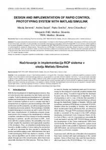
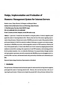
accumulated extra-precisely and rounded back to input/output precision after massive cancellation has taken place. Sometimes Y = X ; sometimes B is diagonal or triangular. Such residuals can be computed from one call to a matrix–matrix–product (GEMM) that accumulates extra-precisely, but a lot of memory traffic can be avoided if versions of GEMM that accept and produce extra-precise matrices are available too (Feature 4: Extra-wide variables). Iterative refinement of nonsymmetric eigenproblems, other than Schur decompositions, depends crucially upon how well iterative refinement works for nearly singular linear systems. For best results, the LU factorization should ideally be performed by Crout factorization with extra-precisely accumulated scalar products, but how much good this would do is not yet clear. Exception handling (Feature 5) is important too because infinity and 0/0 turn up in the better mathematical algorithms mentioned above unless entirely algebraic computations are replaced in spots by invocations of transcendental functions elementwise upon arrays. The last question remaining is how much precision would be needed to perform an entire eigencalculation by conventional means, without refinement, to obtain results as good and as soon as are obtained from refinement with a little extra-precise arithmetic in the program; experience indicates that a high precision conventional algorithm without refinement is much more expensive than with refinement. 2.2.1 Numerical Example. In this section, we study a (well-known) numerical example illustrating the benefits of extra-precise iterative refinement. We used the linear system (LHn )x = (Lb), where Hn is the Hilbert matrix of dimension n, b is the j th column of the identity matrix (which we denote by I j in the figures), and L is a scale factor chosen so that LHn and Lb have integer entries representable without round-off. The Hilbert matrix H has elements hi j = 1/(i + j − 1). We chose the Hilbert matrix because (1) it is very sensitive to roundoff errors, with condition numbers increasing rapidly (see Table I [Higham 1996, p. 516]), and (2) its inverse is known exactly and so we can compute the true solution. L is the least common multiple of all the i + j −1, 1 ≤ i, j ≤ n. Figures 1, 2, and 3 show the convergence history of iterative refinement, with progressively increasing n. We use both the LAPACK routine SSPRFS (single precision, symmetric and packed) and our modification to it with SSPMV replaced by our extended precision version. For the extended precisions, we only plot the extra precision result (ε ≈ 4.93e-32), but not the double precision result (ε ≈ 1.11e-16), because the double precision plots are visually indistinguishable from the extra precision ones. In this experiment, we let the code run 20 iterations, because the examples are very ill-conditioned with respect to single precision (ε ≈ 5.96e-08). In practice, one or two iterations often suffice. In each figure, we plot five quantities (kvk∞ ≡ maxi |vi |). ACM Transactions on Mathematical Software, Vol. 28, No. 2, June 2002.

•


2

Single precision iterative refinement: L * H6 * x = L * I5

10

10

10 FERR BERR ||Xtrue – X||/||Xtrue|| ||dXi||/||Xi|| ||dxi+1||/||dxi||

0

10

Extra precision iterative refinement: L * H6 * x = L * I5

2

FERR BERR ||Xtrue – X||/||Xtrue|| ||dXi||/||Xi|| ||dxi+1||/||dxi||

0

−2

−2

10

10

−4

−4

10

10

−6

−6

10

10

−8

−8

10

10

−10

10

161

−10

2

4

6

8

10

12

14

16

18

20

10

2

4

6

8

10

12

14

16

18

20

Fig. 1. Iterative refinement results in single and extra precision, n = 6, j = 5. Single precision iterative refinement: L * H7 * x = L * I5

4

10

10


2

10

0


2

0

10

−2

−2

10

10

−4

−4

10

10

−6

−6

10

10

−8

−8

10

10

−10

10


4

10

−10

2

4

6

8

10

12

14

16

18

20

10

2

4

6

8

10

12

14

16

18

20

Fig. 2. Iterative refinement results in single and extra precision, n = 7, j = 5.

(1) Forward error bound FERR on x computed by LAPACK (see Demmel [1997] for the derivation): k|A−1 |(|r| + nε(|A||x| + |b|)k∞ kx − xtrue k∞ ≤ FERR ≡ , kxk∞ kxk∞ (2) Componentwise relative backward error [Demmel 1997], computed by LAPACK, which is the smallest relative perturbation in each matrix entry necessary to make the computed x the exact solution of the perturbed problem: BERR ≡ max i

|r|i , (|A| |x| + |b|)i


•

162

X. S. Li et al.

Single precision iterative refinement: L * H8 * x = L * I5

4

10

10

10


2

10

0

10


2

0

−2

−2

10

10

−4

−4

10

10

−6

−6

10

10

−8

−8

10

10

−10

10


4

−10

2

4

6

8

10

12

14

16

18

20

10

2

4

6

8

10

12

14

16

18

20

Fig. 3. Iterative refinement results in single and extra precision, n = 8, j = 5.

(3) The true error kxtrue − xk∞ /kxtrue k∞ , (4) the normalized change in x between successive iterations kxi+1 − xi k∞ / kxi k∞ , and (5) the ratio of changes of x between successive iterations kxi+2 − xi+1 k∞ / kxi+1 − xi k∞ . In the labels in the figures, we let dxi = xi+1 − xi . In Figure 1, four error measures become exactly zero after three or four steps, so nothing is plotted afterwards. From this experiment, we made the following observations: —The single precision iteration can effectively reduce BERR to near ε, although it is slightly worse than the extended precisions. But it cannot reduce the true error of the solution. —Both double and extra precisions can reduce the true error to near ε when the condition number is comparable to or less than 1/ε (when n = 6 or n = 7 but not n = 8). Using more than double, the input/output precision gives comparable results to just using double the input/output precision. —The error bound FERR is good only when the iterative refinement is performed in single precision. If extended precision is used, FERR may be arbitrarily pessimistic. Instead, kd xi k/kxi k should be used as the error bound. Table II shows the relative errors after 20 steps, when using double precision and varying the dimension n from 3 to 10. This also confirms the theory that the improved iterative refinement always produces accurate solution as long as the condition number is not bigger than 1/ε. ACM Transactions on Mathematical Software, Vol. 28, No. 2, June 2002.


•

163

Table II. Relative Errors after 20 Steps of Iterative Refinement in Double Precision n κ2 (Hn ) kxtrue − xk∞ kxtrue k∞

3 5.2e02

4 1.6e04

5 4.8e05

6 1.5e07

7 4.8e08

8 1.5e10

9 4.9e11

10 1.6e13

0.0

0.0

0.0

0.0

0.0

0.3

1.0

1.1

2.3 Example 2: Avoiding Pivoting in Sparse Gaussian Elimination Sparse Gaussian Elimination is a challenging algorithm to implement efficiently because of the high cost of constructing, traversing and modifying the dynamic data structures that are needed to compute the pivot sequence and resulting fill-in of originally zero matrix entries. This cost is especially acute on distributed memory parallel machines because known algorithms require frequent fine-grained messages, and these are expensive. In contrast, sparse Cholesky is a special case of Gaussian elimination applicable to symmetric positive definite matrices, for which any pivot sequence is numerically stable. Sparse Cholesky has been satisfactorily parallelized because the pivot sequence can be chosen ahead of time (i.e., independent of the values of the nonzero matrix entries, or any intermediate results) to optimize load balance and fill-in, and the data structures and communication patterns can be determined statically and more simply [Gupta et al. 1999]. We would like to have an algorithm as parallelizable as sparse Cholesky but applicable to completely general matrices. To do this we have designed a version of parallel sparse Gaussian elimination called SuperLU DIST Li and Demmel, 1998, 2001] that avoids dynamic pivoting, and so permits the same optimizations as parallel sparse Cholesky. To retain numerical stability, we use a variety of techniques including (1) Prepivoting large matrix entries to the diagonal, √ (2) Substituting tiny diagonal pivots by εkAk (which reduces pivot growth at the price of losing half the backward stability enjoyed by conventional pivoting). Preliminary results, where double precision is used internally to achieve single precision accuracy for the computed results [Li and Demmel 2001], show that the above techniques do ensure satisfactory accuracy on a set of challenging test matrices drawn from applications, and also show large speed-ups on suitably large matrices. If the above techniques do not get adequate accuracy (we encountered only one such matrix in our extensive testing), then the following further techniques can be applied. One is to perform iterative refinement with extra-precise residuals, as in Section 2.2 (Feature 2: Extra internal precision). The second approach is to organize the Gaussian elimination in a left-looking fashion, where each entry is updated by the dot product of the corresponding row of L and column of U. For this update, we can use the new DOT function (or GEMV/GEMM in a blocked algorithm). This only requires Feature 2: Extra ACM Transactions on Mathematical Software, Vol. 28, No. 2, June 2002.

164

•

X. S. Li et al.

internal precision. The third technique is to use this inaccurate LU factorization as a preconditioner to an iterative solver, such as QMR or GMRES. For example, for the matrix mentioned above, we achieved an accurate solution with a few iterations of preconditioned GMRES. 2.4 Example 3: Accelerating Iterative Methods for Ax = b, like GMRES The principle of iterative refinement can be applied to other equation solving methods as well, both linear and nonlinear. Turner and Walker [1992] replace the solution of Ad = r via the LU factorization of A by GMRES(m) [Saad and Schultz 1986] to get the correction d , and solves a linear system arising from a discretized elliptic PDE as accurately as though the entire computation were done in double, but while doing nearly all the work in single and so running much faster. Turner and Walker [1992] point out that their observation could have been applied to any other efficient, restarted iterative solver besides GMRES(m), such as GCR(m) [Eisenstat et al. 1983], etc. The algorithm in Turner and Walker [1992] differs slightly from the one in Section 2.2 in that the right-hand side b, the computed solution x, and the product Ax are kept in extended precision (double in their experiments). In other words, they exploit Feature 4: Extra-wide variables, in addition to Feature 2: Extra internal precision. It is not clear from Turner and Walker [1992] whether they really need extra-wide variables, or whether the general scheme of Section 2.2 is adequate; we suspect that it is. 2.5 Example 4: Mixed Real and Complex Arithmetic LAPACK auxiliary routine CLACRM multiplies a complex matrix A by a real matrix B. It is called by the LAPACK routines for computing eigenvalues and eigenvectors of Hermitian matrices using divide-and-conquer (CSTEDC, CLAED0 and CLAED7), currently one of two fastest available algorithms for large matrices. It is similarly used by the complex SVD based on divideand-conquer. The alternative of promoting B to complex and calling the BLAS CGEMM would cost three times as many floating-point operations (four floating-point multiplications and two additions per solution component, instead of two multiplications). Since this routine is the most time-consuming part of the divide-and-conquer algorithm, it is important that it be fast. Currently, CLACRM is implemented by copying the real part of A to contiguous workspace, calling SGEMM, copying the result back, and repeating this for the imaginary part. It would be simpler and more efficient (by avoiding these data copies) to have a matrix-matrix-product routine that accepted a real and complex matrix (Feature 1: Mixed precision). LAPACK auxiliary routines CLASR and CSROT apply one or more real 2by-2 rotations Ri to a complex matrix A. They are called by the LAPACK routines for computing eigenvalues and eigenvectors of Hermitian matrices using QR iteration (CSTEQR), and by the complex SVD, and are the bottlenecks in these routines, which are currently the fastest available algorithms for small matrices. The alternative of promoting the Ri to complex would again triple ACM Transactions on Mathematical Software, Vol. 28, No. 2, June 2002.


•

165

the cost of the most time-consuming part of QR iteration. Currently these routines are implemented in straightforward (unoptimized) Fortran 77 but could be implemented as optimized BLAS with mixed precision inputs and outputs (Feature 1: Mixed precision). It is possible to define a very large number of mixed precision routines, not all of which are useful. For example, the standard matrix-matrix product routine has five floating-point arguments (it computes α AB + βC). If each argument were independently permitted to have one of the four standard floating point types (single, double, single complex, double complex), then there would be 45 = 1024 different combinations, most of which would never be used. Instead, we have identified a small subset of just 12 mixed precision versions (plus the four conventional versions) to implement; see Section 4. 2.6 Example 5: Using Normal Equations Instead of QR for Least Squares This example uses Feature 4: Extra-wide variables, to implement a faster algorithm for the overdetermined least squares problem, that is, finding the x that minimizes kAx − bk2 . The algorithm that uses the fewest floating-point operations is to form the matrix AT A and then solve the so-called normal equations (AT A)x = AT b by Cholesky factorization. This requires about half as many flops as the alternative QR-based approach when the number of rows m of A is much larger than the number of columns n. The trouble is that using the normal equations instead of QR can effectively square the condition number of the problem, and can lose twice as much accuracy. The remedy is to form and solve the normal equations in twice the input/output precision. Unless the condition number is near 1/ε, this can be much more accurate than the QR-based approach in single precision. If we use more than input/output precision but less than twice as much, the error bound is proportionately more. If m is sufficiently larger than n, and the cost of extra precise arithmetic is less than twice the cost of arithmetic in the input/output precision, then this algorithm will be faster than the existing QR-based algorithm. Preliminary benchmarks on a Pentium Pro indicate that forming and solving the normal equations using 80-bit extended arithmetic can be significantly faster than running LAPACK’s implementation of QR, provided m is much larger than n. For example, with m = 400 and n = 20, the normal equations were three times faster than QR, that is, faster than mere operation counts can explain. For the same m, as n grows, the normal equations slow down with respect to QR, with about equal runtimes at n = 45, and with QR 20 times faster for n = 400. For m = 500 and n = 5, the normal equations were 39 times faster than QR! Here is why the normal equations approach cannot be implemented solely with high precision restricted to internal precision for the BLAS. We need to be able to compute, return, and continue computing with AT A and (AT )b in higher ACM Transactions on Mathematical Software, Vol. 28, No. 2, June 2002.

166

•

X. S. Li et al.

precision. This means that we have to be able to declare variables of these types, not just have anonymous variables. Some languages do not permit declaring such high precision variables. Furthermore, Cholesky requires a square root, although LDLT could be used instead. There is a family of Least Squares problems for which extended BLAS are necessary, but not the declaration of higher precision variables. These are simple three-dimensional nearest-point problems: Find the point in a given line or plane nearest another given line or point. These problems have explicit solutions expressed in terms of scalar- and cross-products [Kahan and Darcy 1998, pp. 48–55]. Many other geometrical problems are solved by computing bilinear and quadratic forms, during which massive cancellation is brought about by near-degenerate configurations that are incidental to the solution of a larger and well-behaved problem. The incidence of geometrically inconsistent results, or instead recourse to higher precision for all intermediate computations, can be diminished by orders of magnitude, sometimes to zero, if BLAS with internal extra precision (Feature 2: Extra internal precision) are used during the computation of those bilinear and quadratic forms. This approach is particularly attractive on computers that can evaluate extended precision BLAS about as fast as ordinary BLAS, as is the case for the overwhelming majority of computers on desktops containing, as they do, Intel or clones inside. 2.7 Example 6: Solving Ill-Conditioned Triangular Systems The LAPACK subroutine SLATRS solves a triangular linear system Tx = scaleb with careful scaling to prevent over/underflow (here scale is an output argument chosen by the algorithm to avoid over/underflow). It is used instead of the Level 2 BLAS routine STRSV when we expect very ill-conditioned triangular systems, and want to get the solution vector (with the scale factor) despite the fact that it may be very large or very small. This is the case with condition estimation (SGECON, SPOCON, STRCON) and inverse iteration to find eigenvectors of nonsymmetric matrices (SLAEIN). SLATRS does careful scaling in the innermost loops to prevent over/underflow, and is significantly slower than an optimized STRSV. Also, it contains about 320 executable statements (versus 160 for the unoptimized version of STRSV), a measure of the complexity of producing such code. There are three ways to accelerate SLATRS. Since the standard interface to the BLAS routine for solving a triangular system does not allow for returning the scale factor, we believe that more than just Feature 3: Wider internal range is needed. The first way is to use Feature 3: Wider internal range along with Feature 4: Extra-wide variables guarantee that over/underflow cannot occur for a given number of iterations of the outermost loop of (lower) triangular solve: Solve L · x = b, where L is lower triangular for i = 1 to n P x(i) = [b(i) − ( i−1 j =1 L(i, j ) · x( j ))]/L(i, i) ACM Transactions on Mathematical Software, Vol. 28, No. 2, June 2002.


•

167

For example, if the entries of L and b are represented in IEEE single, no diagonal entry of L is denormalized, and 80-bit Intel arithmetic is used to implement this algorithm, testing the scaling is needed only once every 64 values of i. In particular, this could be implemented by calling an optimized 80-bit GEMV on blocks of size 64, which would get much of the benefit of the optimized SGEMV. IEEE Double is not so good, since we could only do blocks of 8. Alternatively, we could use scaling code like that in SLATRS to compute the largest block size we could accommodate. This requires information about the norms of columns of L. In the case of SLAEIN, where we call SLATRS many times, the cost of this information is small. In the case of condition estimation, the cost is larger. The second way to accelerate SLATRS uses Feature 5: Exception handling, and was explored in Demmel and Li [1994]. The IEEE exception flags can be used to hide over/underflow problems as follows. We first run using the optimized STRSV, and then check the exception flags. Since over/underflow is rare, this will almost always indicate that the solution is fine. Only in the rare cases that an exception occurs does one need to recompute more carefully. This is definitely the way to go on a Pentium. Speed-ups reported in Demmel and Li [1994] ranged from 1.4 to 6.5. The third way to accelerate SLATRS, which could complement the above ways, is to estimate more cleverly how big a block we can call STRSV on, based on some data about sizes of off-diagonal entries of the matrix. SLATRS currently does this in a naive way, and we have explored better alternatives as well. The complex analog CLATRS is used in the above routines as well as in some other LAPACK routines like CTREVC, which computes eigenvectors of triangular matrices. Speedups of CTREVC using exception handling reported in Demmel and Li [1994] ranged from 1.38 to 1.65. The overall routine CGEEV for the complex nonsymmetric eigenproblem sped up by 8%, since CTREVC is just part of the calculation. 2.8 Example 7: Eigenvalues and Eigenvectors of Symmetric Matrices We discuss the acceleration of methods for computing the eigenvalues and eigenvectors of a symmetric matrix. In particular, they apply to the second phase of the algorithm, when the original matrix has been reduced to tridiagonal form. We use combinations of Feature 3: Wider internal range, Feature 4: Extra-wide variables, and Feature 5: Exception handling. We begin with the recently released LAPACK code xSYEVR [Anderson et al. 1999], which uses a new algorithm [Dhillon 1997; Dhillon et al. 1997; Parlett and Dhillon 1997; Parlett and Marques 2000] that is significantly faster than any previous algorithm, running in O(n2 ) time to find all the eigenvalues and all the eigenvectors of an n-by-n symmetric tridiagonal matrix. The core of the new algorithm is in subroutine xLAR1V, which computes the so-called stationary qd transform of a tridiagonal T in factored form T = LDL T , producing a factored T , where σ > 0 is a shift, D and D+ are diagonal, form of T − σ I = L+ D+ L+ and L and L+ are unit lower triangular and bidiagonal (i.e., L and L+ have ACM Transactions on Mathematical Software, Vol. 28, No. 2, June 2002.

168

•

X. S. Li et al.

ones on the diagonal, nonzeros on the first subdiagonal, and zeros elsewhere). The algorithm is s = −σ for i=1 to n − 1 D+ (i) = D(i) + s L+ (i + 1, i) = L(i + 1, i) · D(i)/D+ (i) s = s · L+ (i + 1, i) · L(i + 1, i) − σ end for D+ (n) = D(n) + s

If the final value of s is Not-a-Number, which may occur if σ is larger than the smallest eigenvalue of T , this is detected (by asking if not(s > 0 or s < 1)) and a slower version of the above loop is run with branches to avoid creation of ±∞ or NaN. The same idea is used to speed up the computation of eigenvalues in the differential qd transform in LAPACK subroutine xLASQ3. The speed-up of the overall routine for finding all the eigenvalues of T by exploiting arithmetic with NaNs and infinities this way ranges from 1.28 times faster on a Sun Ultra 30 to 1.8 times faster on an IBM RS-6000/590 [Parlett and Marques 2000]. This does not require the full power of Feature 5: Exception handling, just IEEE default arithmetic [ANSI/IEEE 1985; ANSI/IEEE 1987]. Similarly, the ScaLAPACK routine PDLAIECT assumes the availability of arithmetic with ±∞ (like 1/∞ = 0) to remove branches from the inner loop in the computation of eigenvalues, and so go faster. The simplest version of the inner loop in PDLAIECT counts the number of eigenvalues less than x of the symmetric tridiagonal matrix T with diagonal entries a(1 : n) and off-diagonals b(1 : n − 1) (we assume b(0) = 0): count = 0 d (0) = 1 for i = 1 to n d (i) = a(i) − x − b(i − 1)2 /d (i − 1) if d (i) < 0, count = count + 1 end for

In practice d (i) overwrites d (i − 1), and we replace the inner loop by d = a(i) − x − b(i − 1)2 /d . The trouble with this is that if d is small or zero, overflow occurs. The standard fix is to test if d is too small, and explicitly set it to a tiny safe value if it is: for i = 1 to n d = a(i) − x − b(i − 1)2 /d if (|d | < too small ), d = −too small if d < 0, count = count + 1 end for

A faster way used by PDLAIECT if the user is on a machine implementing IEEE infinity arithmetic (i.e., most of the time) is to go ahead and compute an infinite d , since the next time through the loop b(i−1)2 /d will be zero, and the recurrence will continue uneventfully. This also requires updating count slightly differently, to account for −0s. Speed-ups reported in Demmel and Li [1994] range from 1.18 to 1.47. This also does not require the full power of Feature 5: ACM Transactions on Mathematical Software, Vol. 28, No. 2, June 2002.


•

169

Exception handling, just the IEEE defaults [ANSI / IEEE 1985, 1987]. for i = 1 to n d = a(i) − x − b(i − 1)2 /d count = count + signbit(d ) end for

The above loop requires neither extra precision nor wider range, and is in fact part of ScaLAPACK [Blackford et al. 1997]. One can further accelerate this recurrence by reorganizing it to remove the division, which can cost six times or more than the other floating-point operations. This loop looks like for i = 1 to n p(i) = (a(i) − x) · p(i − 1) − b(i − 1)2 · p(i − 2) if ( p(i) and p(i − 1) have opposite signs), count = count + 1 end for

The relationship between these loops is that d (i) = p(i)/ p(i − 1). Again we can remove the subscript on p(i) if we use two temporaries. This loop has no division, and so may be much faster than the first one. Not all machines have such slow division, so this will be machine dependent. However, this loop is much more susceptible to over/underflow, because p(i) is the determinant of the leading i-by-i submatrix of T − x I , and determinants easily over/underflow. For example, det(xeye(n)) = x n in MATLAB notation, and neither x nor n has to be very large for overflow to occur. We again have two approaches as in Section 2.7: First, we can use Feature 4: Extra-wide variables, which requires Feature 3: Wider internal range to implement the loop; for example, using 80-bit arithmetic will let us reduce the frequency of scaling tests in the inner loop to one every 128 iterations with IEEE single inputs or 16 with IEEE double. Second, we can use Feature 5: Exception handling to decide when overflow has occurred and (partial) recomputation with scaling is necessary (this may be used in conjunction with Feature 4: Extra-wide variables to reduce the incidence of exceptions). There are various ways to accelerate bisection by using Newton’s method or related ideas, but all involve inner loops similar to the one above. Since PDLAIECT is not a BLAS routine, there is no way to hide the use of Feature 4: Extra wide variables or Feature 5: Exception handling. 2.9 Example 8: Cheap Error Bounds A simple and attractive, if not always rigorously justified, way to get error bounds is to do an entire computation in one precision, say single, and then do it again entirely in a high precision, say double. For simplicity, suppose the true result of subroutine sol ve is the scalar x, and call the single precision scalar answer x S and the double precision scalar answer x D . Then, the simple error bound for the error in x S is simply |x S − x D |. The justification is that if the algorithm is backward stable, then x S can be expressed as x S = x + κε S , where κ is the unknown condition number and ε S is at most single-precision machine epsilon in magnitude. Similarly, x D = x + κε D . Then |x S − x D | = |κ(ε S − ε D )| ≈ |κε S |, the error in x S . The error in x D is roughly ε D /ε S times smaller. There are ACM Transactions on Mathematical Software, Vol. 28, No. 2, June 2002.

170

•

X. S. Li et al.

several ways these estimates can be too large or too small, but they are better than nothing. When x D cannot be computed entirely in double precision, but perhaps only with some parts in double (like the internal precision of the BLAS), then the reliability of |x S − x D | as an error bound decreases, but it still has some value. This makes it attractive to write subroutine solve for computing x with the precision (S or D) as an input parameter. This means just one version of solve would have to be written, and the decision to use single or double precision would be made at run-time. Given the way variables are declared in languages like Fortran and C, we cannot change their types from single to double at runtime, but we can hope to change Feature 2: Extra internal precision, that is, how much internal precision is used within the BLAS. In other words, we could pass in a variable PREC which might equal Single or Double, and in turn pass this as a run-time argument to the BLAS. The alternative, where the internal precision is determined at compile time, would mean that we would need (at least) two versions of solve, or code within solve that branches based on PREC and calls different BLAS routines. This would make solve unpleasant to write, read and maintain. 3. IMPLEMENTATION TECHNIQUES FOR EXTENDED PRECISION 3.1 Introduction Most of the diverse schemes by which hardware, compilers and languages may support the five arithmetic features listed in Section 2.1 are described in this section. The schemes discussed are just the ones deemed most likely to support extended precision BLAS. After a general discussion and history of these techniques, we discuss the implementation used in our reference implementation in more detail. Almost all computer architectures and the programming languages available for them support more than one floating-point format. The two formats supported practically universally are 32-bit = 4-byte single precision and 64-bit = 8-byte double. The CRAY X-MP, . . . , J90 family constitutes the only exception at present and shall be discussed no further. Many architectures and some compilers support a third floating-point format wider than the first two. The basic kinds of extended (beyond double) precision formats that have been supported in hardware, firmware or software are named here in roughly descending order of speed. More details are presented in Sections 3.2 and 3.3. Double-extended. This is a conventional floating-point format with one field each of sign bit, exponent, and significand. ANSI/IEEE Standard 754 requires this format to have at least 15 exponent bits and 64 bits of significand. These requirements are met (barely) by an 80-bit = 10-byte register on most Intel processors and their clones. These processors performs floating-point operations by default in these Double-extended registers even if results are rounded to narrower widths. This makes operations fast in so far as their execution times vary with operands’ widths mainly in the times taken to move them through ACM Transactions on Mathematical Software, Vol. 28, No. 2, June 2002.


•

171

memory, not much in times taken by arithmetic. Except for 11 extra bits of precision, Double-extended arithmetic rounds in the same careful way as does double, so error analysis changes solely because of a somewhat smaller roundoff threshold. Double-double. Each 16-byte operand is the unevaluated sum of two 8-byte doubles of which the first consists of the “leading” digits, and the second the “trailing” digits, of the format’s value. Its exponent range is almost the same as double’s, differing only in some vagueness about underflow, since only one word may underflow at a time. Rounding is vague too; its precision is roughly twice double’s, and its error-analysis rather rough (see Section 3.3.1). Implementation is in software that may be hardware-dependent, though it can be made portable to all processors relevant to this document at the cost of some speed. This issue is important because Double-double is worth using only when it is noticeably faster than Quadruple, as can often occur if floating-point hardware capabilities are exploited fully. These implementation techniques can be extended further to triple- and quadruple-double, but with diminishing efficiency except in special cases [Briggs 1998; Priest 1991; Shewchuk 1997]. These techniques have also P been used to compute dot products (α i xi y i +βr) with all correct leading digits, despite all round-off [Kulisch and Miranker 1983; Bleher et al. 1985; Kahan and LeBlanc 1985]. We will not consider these very high precision implementations further here. Quadruple precision. This is a conventional 128-bit = 16-byte wide floatingpoint format with one field each of sign bit, exponent, and significand, though perhaps stored in two 8-byte words with the second’s exponent field unused. The precision is at least wide enough to hold exactly the product of two doubles. Nowadays, Quadruple precision operations run at least several times slower than double but use the same careful algorithms for rounding, so error-analysis changes solely because of a much smaller round-off threshold. BigFloats. This is not really an extension of floating-point hardware; instead, arbitrarily high precision is accomplished by breaking every number into equal-width “big digits” each stored as an element of an array of integers or integer-valued doubles. This kind of software-simulated floating-point is built into automated algebra systems like Macsyma, Inc. [1996], Mathematica [Wolfram 1988] and Maple [Monagan et al. 1997], and provided to other programmers by packages like Richard Brent’s MP [Brent 1978] and David Bailey’s MPFUN [Bailey 1995]. BigFloats are optimized for very high precision, and run so much slower than Double-double or Quadruple when delivering comparable precisions that BigFloats shall not be treated further in this document. Unfortunately, our three names “Double-extended,” “Quadruple precision,” and “Double-double” need not correspond with the names programming languages use for precisions beyond double. For instance, “TEMPREAL,” “REAL*10,” “REAL*12,” and “REAL*16” are the names used by the few Fortran compilers that support(ed) Double-extended. On the other hand, “REAL*16” in a Fortran compiler can mean any one of those three, and “long double” in a C or C++ compiler can mean any one of those three or just double precision. ACM Transactions on Mathematical Software, Vol. 28, No. 2, June 2002.

172

•

X. S. Li et al. Table III. Higher-than-Double Precision Formats Available in Hardware

Format Type Double-extended IEEE 754 binary 64 sig. bits

Double-double 2 × 53 sig. bits

Quadruple (Hex) 28 hex digits Quadruple (Binary) 113 sig. bits

Computer Family Intel x86/87 & Pentium PC & clones by AMD, Cyrix. Motorola 680x0-based Apple Macintosh, NeXT, SunIII; Intel 80960KB. HP/Intel IA-64 Itanium; Motorola 88110. IBM RS/6000, Power PC, Apple Power Mac; HP 8000 & PA RISC 2.0; (HP/Intel IA64 Itanium) (IBM s/390 G5) (SGI MIPS) IBM S/370, 3090, S/390. DEC VAX “H”, (Compaq Alpha) IBM S/390 G5 ; (Sun SPARC, HP PA RISC, HP/Intel IA 64, SGI MIPS)

Bytes Width 10

Sig. Dec. 19 – 20

log10 (Overflow) 4932

12

19 – 20

4932

16

19 – 20

4932

16

grubby 32

308

16

31 – 33

76

16 16

33 – 34 33 – 34

4931 4932

The names “EXTENDED” and “quadruple” have also been used by compilers written for hardware with built-in Quadruple precision even if it is vestigial, existing only as unimplemented op-codes that would trap to software if the compiler did not circumvent trap overheads by invoking the software directly. But by conforming to the minimum requirements of a standardized language like Fortran 77, many a compiler denies access to whatever extended precision does exist in the hardware or, worse, uses that extended precision whimsically to evaluate some floating-point subexpressions while disallowing mention of it, as used to happen on the Sun III. Consequently, of the three kinds of extended precision named, only a suboptimal implementation of Double-double can be made portable across all compiler and hardware boundaries. To standardize extended precision BLAS we shall have to cope with diverse formats, implementations, speeds and linguistic impediments. Section 3.2 presents a little more history of the support (or lack of it) for extended precisions. Section 3.3 discusses design options for implementing double-double arithmetic, and finally Section 3.3.2 discusses our implementation, which is based on the Fortran 95 double-double package [Bailey 2000]. 3.2 A Little More History of Extended Formats Among computers still (or once) commercially significant in the world of floating-point computation, many provide(d) more than nominal support for a third floating-point format wider than the nearly ubiquitous “REAL*4 (float)” and “REAL*8 (double)” formats. Table III lists some hardware supports for higher-than-double precision formats. The term “Extended” first came into widespread association with “Precision” in late 1967 when the IBM S/360 model 85 came out with hardware to support ACM Transactions on Mathematical Software, Vol. 28, No. 2, June 2002.


•

173

addition, subtraction and multiplication (not division) of Quadruple precision hexadecimal floating-point operands. This hardware was IBM’s response to NASA’s expressed but misperceived need for precision beyond double during orbit calculations. IBM’s hardware competed against Seymour Cray’s CDC 6600, whose “single precision” word was 60 bits wide with 48 significant bits of precision; the model 85 also had three peculiar “DX” operations to speed up software-implemented “double precision” (actually “single-single”) with almost 96 significant bits, much wider than IBM’s S/360 double precision with 14 hex digits (about 53–56 significant bits). The mod 85’s “Extended” format persists today, fully supported (including division) in IBM’s S/390 hardware and compilers for it, stored as two 8-byte double precision hex floating-point words superficially resembling Double-double; however, the second word’s sign and exponent are ignored during operations, and its significand may be unnormalized. In the mid 1970s, to provide a functionality competitive with IBM’s “Extended” for the DEC VAX a few years after its debut, DEC augmented its floating-point instruction set with the “H” format, a true Quadruple precision binary format with 113 significant bits of precision in a 16 byte word. DEC’s compilers, plus an excellent mathematical library, supported this format fully though it ran “hot” (in hardware), “warm” (in microcode) or “cold” (in software) on various VAX models, and “cold” on the DEC (now Compaq) Alpha. For several years an almost identical de facto standard Quadruple precision format has existed in several microcomputer architectures that conform to ANSI/IEEE Standard 754 for Binary Floating-Point [ANSI / IEEE 1985]. This format has 15 exponent bits and 113 bits of significand in a 16 byte word, so it qualifies as an ANSI/IEEE 754 Double-extended format with more than the minimum (64 bits) of required precision. At this time only the recent (1999) IBM S/390 G5 processor supports it fully in hardware; it is implemented in software on the HP PA RISC, Sun SPARC, SGI MIPS and HP/Intel IA 64 (Itanium) processors, and accessible through their respective manufacturers’ compilers, though not always accompanied by a fully accurate mathematical library of elementary transcendental functions. The history of extended precisions is littered with sad stories. One is the dearth of language support for extended precisions except in compilers produced under the aegis of hardware manufacturers; where this support has existed its variability detracted from software portability. Perhaps C99 [ISO/IEC 1999] will remedy this deficiency. Another sad story resembles the vicious circle surrounding the division operation: No matter whether implemented “hot” (in hardware), “warm” (in microcode), or “cold” (in software), Quadruple has always run at least several times slower than Double (as dovision has almost always run several times slower than multiplication). Laggardly performance discourages programmers from exploiting Quadruple (and division). Consequent low-duty cycles and (near-)absence from benchmarks provide little incentive for hardware manufacturers to speed up implementations. Moreover, whenever a faster implementation of a hardware architecture has come to market with cheaper but, relative to other operations, slower Quadruple (or division), scarcely any customer has complained or declined to buy on that account. Meanwhile, extended precisions have been shunned for over three ACM Transactions on Mathematical Software, Vol. 28, No. 2, June 2002.

174

•

X. S. Li et al.

decades by expert developers of portable numerical software libraries like EISPACK [Smith et al. 1976], LINPACK [Dongarra et al. 1979], LAPACK [Anderson et al. 1999], and ScaLAPACK [Blackford et al. 1997]. A compromise, to offer programmers some benefits of extra precision and thus enhance the reliability of their numerical software, insinuated a few digits of extra precision into a few places in the hardware’s architecture where performance would not be degraded too much if at all. This compromise appeared in the late 1960s in the accumulator register of GE 635 mainframes (subsequently taken over by Honeywell), then in the floating-point register file of Prime minis, then in the DEC VAX’s EMOD instruction in the early 1970s, then in the internal registers (inaccessible to most users) of HP handheld calculators and decimal computers after 1975. These extra digits were at first intended for use solely in assembly language or microprogramming, so they did not appear in higher-level languages. This linguistic mindset contributed to more sad stories later. In 1977, the 8087 floating-point coprocessor for Intel’s 8086/88 processors was being designed to serve a market that was bigger by orders of magnitude than the computing industry had served before. This vast market’s average level of numerical expertise was expected to be lower than before so, for the sake of enhanced reliability, the 8087 was designed to support three floating-point formats: 4-byte single precision, 8-byte double precision, and 10-byte Double-extended precision with three more exponent bits and eleven more bits of precision than double. Most important, all the 8087’s registers had this extended width, and all operations were carried out to this width regardless of the operands’ precisions, much as the original Kernighan-Ritchie C on DEC PDP-11s had evaluated all floating-point subexpressions in double, regardless of the declared variables’ precisions. In short, applications programmers were intended to use the 8087’s Double-extended precision (Intel called it “TEMPREAL”) for all local variables and intermediate expressions except perhaps large arrays, since the use of narrower precisions could save appreciable time only while they moved through the memory system. By 1981, a proposed IEEE Standard 754 had grown out of the 8087’s design, and its three formats’ rationale and intent had been adopted at three more companies: Motorola was working on the 68881 floating-point coprocessor for its 68020, Zilog on the Z8070 for its Z8000; and Apple had incorporated all three formats into its Standard Apple Numeric Environment (SANE), first for the Apple III’s Pascal and then for the 680x0-based Macintosh and retrofitted for the Apple II. With their eyes on that vast mass market, these three companies designed the Double-extended format to be the default for all floating-point operations. However, there was another market, the one then served by mainframes and minicomputers, to which upscale workstations could be sold with higher speeds and mark-ups than were contemplated for the mass market of Personal Computers. Workstation users were expected to recompile many of their mainframe applications, which hardly ever mentioned Extended. Since they cared about speed to the near exclusion of everything else, the draft of IEEE 754 left the Double-extended format to the implementor’s option. By 1982–1983, implementations of IEEE 754 without that option were under way ACM Transactions on Mathematical Software, Vol. 28, No. 2, June 2002.


•

175

at National Semiconductor, Weitek, Sun SPARC, MIPS (now SGI), and IBM, whose RS/6000 processor, developed in Austin, Texas, evolved into the Power PC now produced also by Motorola and used in MACS. By 1985, when IEEE 754 was promulgated as an official standard, two versions of it had become de facto standards for most new computer hardware. All three of its floating-point formats were supported by a few numerically superb compilers for SANE on Apple Macintoshes; but most compiler makers continued to use front ends that lacked names for a third floating-point format, so they catered to only the minimal version of IEEE 754 with just single and double. Short-term marketing priorities overruled long-term mathematical considerations. In 1980, for instance, Microsoft was implementing compilers for the forthcoming IBM PC, which had an Intel 8088 processor and a socket for the 8087. Microsoft wrongly prophesied emptiness for almost all of those sockets, so its compilers lacked support for Double-extended arithmetic which, in software, would have run somewhat slower than double. Later, when Borland came out with Pascal and C compilers that supported all three floating-point types, Microsoft followed suit for a decade until, by the late 1990s, its dominance of the market let it drop support for Double-extended from its compilers run on Windows NT, which was implemented originally on DEC Alphas whose IEEE 754 arithmetic had only single and double. Apple’s alliance with IBM in the late 1980s entailed switching Macintoshes from the 680x0 to IBM’s Power PC. Because it supported only single and double precisions, this choice of processor scuttled SANE. It need not have happened that way; other fast RISC processors like Intel’s 80960KB and Motorola’s 88110 could have sustained SANE. But floating-point did not figure in Apple’s marketing plans. Currently 10-byte Double-extended is practically ubiquitous in the hardware of Intel x86/87 and Pentium processors and their clones by AMD and Cyrix. The width of this format may be padded by extra bytes to avoid memory alignment delays and allow for future growth to a wider significand if and when market conditions demand it; the total padded width is 12 bytes for Motorola 680x0/68881/2 and Intel 80960KB and 16 bytes for Motorola 88110 and HP/Intel IA 64 (Itanium) processors. All these processors can evaluate floating-point operations by default in Double-extended registers, even if results are rounded to narrower widths; their execution times vary with operands’ widths mainly in the times taken to move them through memory, not much in times taken by arithmetic. However, even if some Microsoft compilers use it surreptitiously, they stopped supporting Double-extended when Windows NT came out. Java does not support it at all, and no commercially significant Fortran compilers support it. Maybe things will change with the emergence of C99 and Itanium. The first and easiest way for BLAS to exploit Double-extended on hardware that has it is to use it to accumulate scalar products and matrix products of double precision data. There is ample precedent for extra-precise accumulation; products of single precision matrices used to be accumulated in double precision routinely until the mid-1960s when doing so became slow on CDC mainframes and inconvenient on IBM mainframes because standard Fortran semantics had been changed. The superior quality of results obtained by ACM Transactions on Mathematical Software, Vol. 28, No. 2, June 2002.

176

•

X. S. Li et al. Table IV. Conflicting Product Lines with and without Double-Extended Vendor Apple Compaq HP IBM SGI Sun Microsoft

Line(s) with double-extended Old 680x0-based Macintosh Wintel PC Wintel PC, IA-64 Wintel PC Wintel PC Solaris on Intel-based PC Windows 9x on PC

Line(s) without Power Mac, iMac DEC Alpha HPUX on PA RISC Power PC, RS/6000 UNIX on MIPS R-x000 Solaris on SPARC Windows NT on DEC Alpha

LAPACK and MATLAB for large-dimensional and ill-conditioned problems would distinguish hardware capable of extra-precise accumulation advantageously from others [Kahan 1998]. Versions of MATLAB that ran on old 680x0-based Apple Macintoshes, and old versions of MATLAB running on Wintel PCs, delivered matrix products more accurate thereon than MATLAB used to deliver on upscale Sun SPARCs and SGI MIPS, or delivers now on all computers. Mathematica’s N[ . . . ] operator delivered three more decimal digits’ accuracy on old MACS and NeXTs than on all other computers. Should ostensibly portable software be allowed to get better results on some hardware than on others? The answer “Yes” seems obvious to the owners of the better hardware, but not so clear to software developers who yearn for Java’s promise of identical floating-point results for everybody everywhere even if it is a pipe-dream. Each variation multiplies the cost of software testing and validation. On the other hand, “no variation” implies “no change,” which stifles evolutionary progress, leaving no alternative but revolution. Voltaire put the conflict succinctly: “The Better is the enemy of the Good.” It will not be resolved here. The tension between knowledgeable purchasers of computing platforms (hardware and operating systems) on the one hand, and applications software vendors on the other hand, poses dilemmas for platform vendors whose different product lines offer different floating-point qualities. Table IV shows some of the vendors who must cope with invidious comparisons and conflicting loyalties within their own houses. In Windows NT on a PC, the conflict was resolved highhandedly by inhibiting the PC’s Double-extended to match the DEC Alpha’s arithmetic limitations. Java seems to be attempting the same for the sake of Sun’s SPARC. Other vendors may have to exercise greater sensitivity to market conditions. The outcomes of these conflicts will not be predicted here except for the wry observation that, by itself, technical superiority cannot ensure market success despite what R.W. Emerson may have said about a better mousetrap. Finally, we mention that G. Henry built a comprehensive software suite of scalar extended precision operations for ASCI Red, which consists of Pentium Pro processors running Linux [Henry 1998]. It includes object code in ELF format, and so is callable from C or Fortran on Linux-based Intel-inside workstations, and perhaps Solaris X86, though this remains to be determined. A typical routine is xadd YYY (a,b,c), which computes a = b + c. Each Y indicates the type of a (first Y), b (second Y) or c (third Y), which can independently be single (“s”, 32 bit), double (“d”, 64 bit), extended (“x”, 80 bit), or even double-double ACM Transactions on Mathematical Software, Vol. 28, No. 2, June 2002.


•

177

(“w”, 128 bit) and double-extended–double-extended (“q”, 160 bits) (discussed in the next section). In other words, there are 53 = 125 add functions. Other operations are subtraction, multiplication, mul-add, mul-subtract, sqrt, assignment (conversion), and reciprocation. There is also a dot product that takes doubleprecision input vectors and accumulates the dot product in extended. Finally, there are routines to change the rounding mode to 64-bits or 80-bits, and to print a number. There are over 700 routines, which were produced with the help of an automatic generation tool. This shows that an implementation that completely supports all kinds of mixed precision operations will be very large, and require automation to build and support. 3.3 More about Double-Double The 16-byte Double-double format can be implemented in portable software to run on all machines that conform to ANSI/IEEE 754 and on quite a few that don’t, and runs about an order of magnitude slower than double but usually considerably faster than Quadruple. Double-double and its variations have an extensive history, with implementation ideas going back to the 1960s [Pichat 1972; Dekker 1971; Kahan 1968; Møller 1965; Priest 1991; Shewchuk 1997; Briggs 1998; Henry 1998; Bailey 2000]. See especially Priest [1991] for a history. Our implementation is based on Bailey’s double-double package [Bailey 2000]. The routine for adding two double-doubles (ddadd) is shown in Figure 4 as an illustration. This algorithm requires 20 floating-point operations. For all the other algorithms with various combinations of inputs and outputs, see Li et al. [2000]. Double-double can be sped up roughly twofold if advantage is taken of a Fused Multiply-Accumulate (FMAC) operation on hardware that has it. This operation computes expressions like X ∗ Y + Z , X ∗ Y − Z and Z − X ∗ Y with just one rounding error at the end instead of two rounding errors, one after multiplication and another after addition. (Do not confuse the FMAC with the unfused MAC operation that computes X ∗ Y + Z in one instruction but with two rounding errors, thus saving only time.) The FMAC appeared first in 1984 on the IBM RS/6000, whose reduced instruction set designed two decades earlier by Dr. John Cocke had only three floating-point operations: conversions between single and double precision, and a MAC. This MAC was upgraded to an FMAC when it was found necessary for a software implementation of division correctly rounded at a tolerable speed. Among many other uses, the FMAC accelerates double-double by computing exactly a product X ∗ Y of two doubles in just two operations, thus drastically shortening the double-double multiplication algorithm: P := X ∗ Y + 0 rounded to double; Q := X ∗ Y − P exactly as a double thanks to the FMAC. Now the product of X and Y equals the sum of doubles P and Q exactly, although rounding that sum to double would yield just P . This kind of unevaluated sum of a leading and a trailing double is the way every doubledouble is represented by a pair of doubles. To compute P and Q without an ACM Transactions on Mathematical Software, Vol. 28, No. 2, June 2002.

•

178

X. S. Li et al.

void ddadd(double dda[2], double ddb[2], double ddc[2]) { /* Compute double-double = double-double + double-double (ddc = dda + ddb). */ /* dda[0] represents high-order word, dda[1] represents low-order word. */ double bv; double s1, s2, t1, t2; /* s1 bv s2

Add two high-order words. */ = dda[0] + ddb[0]; = s1 - dda[0]; = ((ddb[0] - bv) + (dda[0] - (s1 - bv)));

/* t1 bv t2

Add two low-order words. */ = dda[1] + ddb[1]; = t1 - dda[1]; = ((ddb[1] - bv) + (dda[1] - (t1 - bv)));

s2 += t1; /* Renormalize (s1, s2) t1 = s1 + s2; s2 = s2 - (t1 - s1);

to

(t1, s2) */

t2 += s2; /* Renormalize (t1, t2) */ ddc[0] = t1 + t2; ddc[1] = t2 - (ddc[0] - t1); } Fig. 4. Adding two double-doubles.

FMAC would cost six conventional multiplications plus several additions or subtractions. The FMAC is built into the hardware of IBM’s RS/6000 and, for compatibility with it, into the S/390 G5 processor as well as the IBM/Motorola Power PC used in Apple’s Power MACS. The same goes for HP’s 8000 and PA RISC 2.0, and for the SGI MIPS R-8000. At present C99 [ISO/IEC 1999] is the only higher-level programming language that offers an explicit invocation fma(x, y, z) = x ∗ y + z of the FMAC. Language support for the use of FMACs by default on hardware that has it poses problems partly because of ambiguity (how should “X ∗ Y + A ∗ B” be evaluated?) and partly because indiscriminate use can, in very rare instances, break programs that would have worked well with an unfused MAC. Because of these rare instances, MATLAB eschews the FMAC. Worse, the MIPS R-10000 uses the same opcode for its unfused MAC as the ACM Transactions on Mathematical Software, Vol. 28, No. 2, June 2002.


•

179

R-8000 used for its FMAC, thus dropping conundrums in the way of language support. The HP/Intel IA 64 Itanium has a Double-extended FMAC that can serve double-double and double-double-extended with the same algorithms, and perhaps serve software-implemented Quadruple too. The IEEE Floating Point Standards committee is considering how to standardize the FMAC instruction in their planned revision of the IEEE Floating Point Standard [ANSI/IEEE 1985; IEEE 2001]. Here are some other double-double implementation efforts. Briggs [1998] released a C++ class library implementing a doubledouble type. It lets users declare double-double variables and operate on them using standard infix operators via operator overloading. It supports the usual four arithmetic operations, sqrt, transcendentals, and I/O. In other words, it essentially makes double-double a first class floating-point data type, so that one could use it internally to the BLAS or externally. It runs on the X86 architecture with Linux and GCC, X86 with Windows 95 and Microsoft C++, MIPS with IRIX and EGCS, and SPARC with Solaris and EGCS. Bailey [19XX] released a Fortran 95 double-double package. It does not introduce a new data type for double-double variable, but just represents it using a pair of REAL*8 numbers. It supports the usual arithmetic operations and transcendental functions. It is portable on all the machines with IEEE floating-point arithmetic. In fact, our double-double implementation and basic algorithms are very similar to Bailey’s, modified as described in the next section. Finally, Henry’s [1988] package mentioned above includes not just doubleextended operations, but double-double and double-extended–double-extended (i.e., 160-bits, with 128 fraction bits). 3.3.1 Why Double-Double is an Attractive Nuisance Except for the BLAS. Currently, machines with an FMAC run double-double a few times faster than correctly rounded Quadruple implemented in software. This speed advantage turns double-double into an “attractive nuisance,” like an unfenced backyard swimming pool. The trouble grows out of the diverse ways double-double can be rounded, none of them strictly correct. An outline of the trouble, which only occurs when we try to use double-double more widely than inside the BLAS, goes like this: Consider a Pascal, Fortran or C Function F (X ) written “polymorphically” in four versions, the first using exclusively small integer constants and REAL*4 (float) variables, the second the same except for replacement of every REAL*4 (float) by REAL*8 (double), the third the same but for REAL*10 (Doubleextended or TEMPREAL), and the fourth the same but for REAL*16 (long double). This program is intended to approximate some ideal real function f (x) that can be inferred from F (X ) by substituting “INFINITE PRECISION” for every “REAL* · · · ” declaration and attending to a few technical details concerning stopping criteria for iterations. For instance, the rounding error threshold EPS/2 should be gauged from statements like T := 3 ; EPS := ABS(1 + 3 ∗ (1 − 4/T )) ; ACM Transactions on Mathematical Software, Vol. 28, No. 2, June 2002.

180

•

X. S. Li et al.

(only the quotient should be inexact); and convergent iterations that would take infinitely many repetitions to achieve infinite precision should be assumed to do so instantly. If each of the first three versions of F (X ) matches f (x) within a few units in the last place of the precision declared for F (X ), then we may well expect the same for the fourth version, and this expectation is fully justified if REAL*16 (long double) compiles to correctly rounded Quadruple precision or even just Double-extended. But not if it compiles to double-double; then program F (X ) can malfunction arbitrarily badly. These malfunctions are not mere theoretical possibilities; they do happen, rarely but not rarely enough to ignore, on IBM’s and Apple’s Power PCs, whose compilers support double-double fully as well as IEEE 754 single and double precisions. Consequently there is some non-negligible risk of malfunction if a program recompiled for those machines was imported from machines, like IBM’s S/390 G5, on which “REAL*16” means Quadruple precision, or from machines like old MACS, on which “long double” meant Double-extended. The risk for BLAS is probably negligible, arising perhaps from none but contrived situations; still, the risk deserves some discussion. The quantity EPS computed above is the gap between 1.0 and the next bigger floating-point number in the format to which 4/T was rounded unless this format is double-double, in which case the gap is far tinier. When computed in Double-IEEE-754-double, EPS comes out to be 2−106 provided division and subtraction are rounded with care; but 1.0 + 2−1022 is a doubledouble number much closer to 1.0. More generally, most double-double precision numbers X are separated from their neighbors by gaps of the order of X ∗ EPS; but around double precision numbers the double-doubles are much denser, some separated by gaps no bigger than the smallest positive double, 2−1074 for Double-IEEE-754-double. Consequently a rounding error in doubledouble can vastly exceed the gaps between adjacent numbers. This disparity breaks the logic and validity of some error analyses valid for conventional floating-point. Here is an example. A common way to approximate cosh(x) is to compute Z = EXP(ABS(X )) (rounded to roughly working precision) and then COSH(X ) = (Z + 1/Z )/2. Let us ignore overflow. Then COSH(X ) may well be less accurate than correctly rounded, yet it is provably monotonic in this sense: COSH(X ) > COSH(Y ) implies ABS(X ) > ABS(Y ). This is provable for every binary floatingpoint format conforming to IEEE 754/854. But not for double-double; no matter how carefully it is implemented, it almost certainly violates that monotonicity relationship for some smallish arguments X and Y . Here is another example. Suppose the iteration x → f (x) converges at a tolerable rate in a monotonically decreasing way to a finite limit L. Then the loop X := initial guess, certainly too big ; Y := anything bigger than X ; while X < Y do Y =X ; X = F (Y ) ; end while L := Y ; ACM Transactions on Mathematical Software, Vol. 28, No. 2, June 2002.


•

181

is a reasonable way to compute L as fast as possible about as accurately as the arithmetic allows. But not in double-double. If unluckily the limit L is representable exactly in double precision, then the sequence of iterates X can look like L + 2−100 , L + 2−101 , L + 2−102 , . . . , L + 2−1074 before it stops. That takes far longer than may have been expected. Worse, a loop not so different from this one is often used to reveal at run-time a conventional arithmetic’s rounding error threshold EPS/2 by seeking the smallest increment D that increases the computed value of 1+D. For double-double, such a loop sets D near the underflow threshold instead of the rounding error threshold. (To get a correct result, substitute “4.0/3.0 rounded to double-double” for “1”.) Hazards like these examples are unlikely to afflict the BLAS though eigensystem calculation may be affected elsewhere, and so may some computations with special structured matrices like Cauchy matrices. On all machines that conform to IEEE 754, double-double can be implemented in a portable way that would give exactly reproducible results, but this is unlikely to persist for long for two reasons: First, an implementation optimal for one architecture may well be very suboptimal for another, especially if the latter has an FMAC the former lacks. Further differences arise if some machines tolerate testing and branching much better than others that run faster if extra arithmetic operations are used in place of tests and branches. Different optimized implementations can give different but roughly equally valid results on different machines. Secondly, implementing double-double differently for the BLAS than elsewhere is worth considering. For example, double-double’s round-off threshold EPS/2 is roughly 2−107 for IEEE 754 double, so one might reasonably expect a difference X − Y of double-double arguments to be computed with an error no worse than something like EPS ∗ |X − Y |. Doing so takes noticeably longer than if instead an error no worse than roughly EPS ∗ (|X | + |Y |) were tolerable, as is almost surely the case for matrix multiplication. Thus, double-double can run sloppier and faster inside the BLAS than outside them. Of course, if it is sloppy outside too, then bad things may well happen faster, starting with the failure of the short formula above for EPS. In short, double-double is an attractive nuisance outside the BLAS but very worthwhile inside them. 3.3.2 Performance of Our Double-Double Implementation. Although the double-double arithmetic operations require many more floating-point operations, these operations are mostly performed at the register level without incurring much more memory traffic. The overall speed of an extra precision BLAS routine is not much slower. To confirm this, we timed several versions of GEMV and GEMM routines on a Sun UltraSPARC, with 333 MHz clock rate and 2 Mbytes secondary data cache. The peak Megaflop rate is 666 Mflops. The performance results are presented in Figures 5 and 6. The routines we have ACM Transactions on Mathematical Software, Vol. 28, No. 2, June 2002.

182

•

X. S. Li et al.

timed are the following: (1) c dgemv (c dgemm): our GEMV (GEMM) with double precision for everything, (2) c dgemv x (c dgemm x): our GEMV (GEMM) with double precision input/output, and double-double internal precision, (3) f77 dgemv (f77 dgemm): the Fortran 77 double precision GEMV (GEMM) from Netlib, and (4) sun dgemv (sun dgemm): the double precision GEMV (GEMM) from the Sun Performance Library. Without extra precision, our GEMV and GEMM run at about the same speed as the Fortran versions. That is, the c dgemv/c dgemm curves are essentially the same as the f77 dgemv/f77 dgemm curves. The GEMM from the Sun Performance Library can be much faster than ours and the Fortran version for large matrices; this is because we have not performed any optimizations to improve data locality, such as blocking. That is, the c dgemv/c dgemm curves are essentially the same as f77 dgemv/f77 dgemm curves, see Figures 5(a) and 6(a). For the extra precision routines, when the matrices are small and all fit in cache, we observed about a factor of 9 to 10 slowdown. When the matrices are large and do not fit in cache, we observed only about a factor of 3.6 slowdown, see Figures 5(b) and 6(b). We also plot Megaflop rates in Figures 5(c) and 6(c). The flop counts for the normal GEMV and GEMM are n(2n + 3) and n2 (2n + 3), and for the extra precision versions are n(37n + 62) and n2 (37n + 62). The extra precision routines achieve a sustained performance of 270 to 300 Mflops for both GEMV and GEMM, showing excellent data reuse even without any algorithmic blocking. Indeed, the Megaflop rates for the extended precision codes are so high that for some applications further tuning may not be needed. But for some other applications, we believe some code optimizations may make a significant impcat in speed. For a standard model of floating-point arithmetic, fl(a ¯ b) = (a ¯ b)(1 + δ),

in the absence of over/underflow,

(1)

where ¯ ∈ {+, −, ×, /}, we can show that our double-double algorithms yield |δ| bounded by 2 · 2−106 (for +), 4 · 2−106 (for ×) and 4 · 2−106 (for /), respectively. This is more than adequate to satisfy the error bounds described in Section 6. We note that there is a more relaxed model of floating-point arithmetic for addition and subtraction fl(a ± b) = a(1 + δ1 ) ± b(1 + δ2 ) satisfied by machines without guard digits, like old Crays, which can be implemented in double-double more efficiently than the stricter model (1). In this relaxed model, the double-double addition (ddadd) algorithm can be considerably simplified. For example, Bailey’s implementation of addition [Bailey 2000] satisfies this model, with |δ1 |, |δ2 | bounded by 2−106 . His algorithm ACM Transactions on Mathematical Software, Vol. 28, No. 2, June 2002.

•

Basic Linear Algebra Subprograms (BLAS) (a) dgemv (row major) [Sun UltraSparc, 333 MHz]

(b) Time ratio of c_dgemv_x over c_dgemv [Sun UltraSparc, 333 MHz]

0.14

0.12

183

12 c_dgemv c_dgemv_x f77_dgemv sun_dgemv

11

10 0.1

9

Ratio

Time (Seconds)

8 0.08 7

0.06 6

5

0.04

4 0.02 3

0

0

100

200

300

400

500 600 700 800 900 Matrix Size (c) dgemv (row major) [Sun UltraSparc, 333 MHz]

1000

2

0

100

200

300

400

500 600 Matrix Size

700

800

900

1000

350 c_dgemv c_dgemv_x f77_dgemv sun_dgemv

300

250

MFLOPS

200

150

100

50

0

0

100

200

300

400

500 600 Matrix Size

700

800

900

1000

Fig. 5. GEMV performance.

requires only 11 floating-point operations as opposed to 20 for ours. We also measured the speed of a few BLAS routines using Bailey’s double-double algorithms. For example, GEMV runs about 35–40% faster. For the sake of speed, BLAS implementors may feel free to use this relaxed model, since it is still adequate to meet the error bounds described in Section 6. 4. SUMMARY OF DESIGN DECISIONS The list of examples in Section 2 was meant to illustrate the opportunities of the five arithmetic features listed in Section 2.1, and the discussion in Section 3 was meant to illustrate their costs. In this section, we weigh the costs and benefits of these features, and present our design decisions. In particular, our design should satisfy the following goals: Goal 1. be reasonable to implement, Goal 2. support some if not all important application examples, ACM Transactions on Mathematical Software, Vol. 28, No. 2, June 2002.

•

184

X. S. Li et al. (a) dgemm (row major, B transposed) [Sun UltraSparc, 333 MHz]

(b) Time ratio of c_dgemm_x over c_dgemm [Sun UltraSparc, 333 MHz]

140

120

12 c_dgemm c_dgemm_x f77_dgemm sun_dgemm

11

10 100

8 Ratio

Time (Seconds)

9 80

7

60

6 40 5 20 4

0 0

100

200

300

400

500 600 700 800 Matrix Size (c) dgemm (row major, B transposed) [Sun UltraSparc, 333 MHz]

900

1000

3 0

100

200

300

400

500 600 Matrix Size

700

800

900

1000

500

450 c_dgemm c_dgemm_x f77_dgemm sun_dgemm

400

350

MFLOPS

300

250

200

150

100

50

0

0

100

200

300

400

500 600 Matrix Size

700

800

900

1000

Fig. 6. GEMM performance.

Goal 3. be easy to use, Goal 4. encourage the writing of portable code, and Goal 5. accommodate growth as we learn about new algorithms exploiting our arithmetic features. Here are our decisions. (1) We do not require that the user explicitly declare or use any new extended precision data types, that is, we do not use Feature 4: Extra-wide variables. Since these are not supported in a standard way by every language and compiler, we cannot reasonably mandate them here. If we made up conventions (like double-double variables occupying a pair of consecutive double-precision words in Fortran 77) then users would expect us to propose subroutines for all the other operations they might want using these variables (binary arithmetic operations, comparisons, binary-decimal conversion, etc.), which is definitely ACM Transactions on Mathematical Software, Vol. 28, No. 2, June 2002.


•

185

beyond the scope of this committee (violating Goal 1). Furthermore, in languages like Fortran 77 without “data hiding” mechanisms, users might have to modify their data structures significantly and replace all infix operators like + and × with subroutine calls (violating Goal 3). Thus the only extended precision that we mandate is hidden inside the BLAS, and so can be implemented in any convenient machine-dependent way. (2) The above decision mostly satisfies Goal 2, since many of the examples in Section 2 can be implemented without Feature 4. Nonetheless, those examples requiring Feature 4 could be supported when the working precision is single and the extended precision is double. This would violate the long-held goal in libraries like LAPACK to be able to run essentially the same code in all available precisions, creating all versions automatically from one single precision template. But it is worth it for the benefits in single. (3) Since we cannot predict all the future applications of extended or mixed precision, nor can we predict what new class libraries or modules will become available to support new data types (e.g., see Section 3.3), it is important to accommodate growth (Goal 5). We do this by making our design as orthogonal as possible to the rest of the BLAS Standard, showing how to take any BLAS routine (including future ones with, say, quadruple precision inputs and outputs), determine whether extra precision is worth using or not, and define the extended precision version if it is. In particular, we believe that extra precision is not worth using unless (1) there is the possibility of cancellation between non-input quantities in the algorithm, and (2) one is not applying orthogonal transformations. The first condition eliminates scaling a matrix by a constant, computing norms of matrices and vectors, and adding two arrays, since in all these cases the result is already good to high relative accuracy without extra internal precision. In fact, adding two numbers to higher precision and then rounding their sum to the lower output precision can yield a very slightly less accurate answer than doing everything in the output precision. The second condition reflects the fact that the orthogonal transformations have already been rounded to working precision, and this does about as much damage to the accuracy as round-off in their subsequent application in working precision to another vector or matrix, so it is not worth making this second step more accurate. (4) Since the number of possible routines with all combinations of mixed precision inputs is very large, and includes combinations unlikely to be used in practice (like multiplying a single-precision-real matrix by a double-precisioncomplex matrix) we specify a small subset of routines that seem to cover most foreseeable needs. In particular, we allow only certain combinations of single real/double real, of single complex/double complex, of single real/single complex, and of double real/double complex. Furthermore, we limit all scalars and output variables to be the “higher” of the two precisions. For example, for matrix-matrix multiplication C = α· A· B+β ·C, the following 12 mixed precisions and types are allowed in addition to the 4 unmixed precision versions (where all arguments are S = single precision real, D = double precision real, C = single precision complex, or Z = double precision complex): ACM Transactions on Mathematical Software, Vol. 28, No. 2, June 2002.

186

•

X. S. Li et al.

α D D D Z Z Z C C C Z Z Z

A S S D C C Z S S C D D Z

B S D S C Z C S C S D Z D

β D D D Z Z Z C C C Z Z Z

C D D D Z Z Z C C C Z Z Z

In other words only 12 out of the possible 45 − 4 = 1020 mixed precision combinations are supported. This satisfies Goals 1 and 2. (5) From Example 8 in Section 2.9, we see that we want to be able to specify the internal precision at runtime; we do this with the variable PREC. This satisfies Goal 3. (6) PREC could potentially take on a great many values, whose meaning varied from machine to machine (see Section 3.3). To achieve Goals 1 and 4, we need to choose a parsimonious subset that will be available on all machines: Single (S), Double (D), Indigenous (I) and Extra (E). If an implementor wants to implement other ones (like triple-double) or indeed if PREC = X (Extended) is supported because it is identical to PREC = I on an Intel machine, that is allowed. Furthermore, if it is easier for the implementor to use more precision than the user requested, that is also allowed. Therefore, provided the inputs are all single precision (real or complex), the only values of PREC that must be supported are S, D, I and E. On any particular machine, this would require at most two or three actual implementations, since either D = I (non-Intel IEEE machines), S = I (some Crays), and/or wider than requested precision may be used (so that S, D and I can all be implemented using I on Intel machines). Our reference implementation provides three versions: a true single precision version when PREC = S, a true double precision version when PREC = D or I, and a double-double version when PREC = E. When the inputs are all double precision (real or complex), the only values of PREC that must be supported are D, I and E. Again, on any particular machine, at most two implementations are needed. On some Crays, I = S is shorter than D (this could be determined safely at run-time via environmental enquiries), so the implementor would use D in place of I on Crays. On nonIntel IEEE machines, D = I. On Intel machines, D can be implemented using I. Our reference implementation provides two versions: a true double precision version when PREC = S, D or I, and a double-double version when PREC = E. So the only really new implementation is PREC = E, which could either be implemented using double-double (as in our reference implementation) or native quadruple (if it exists). ACM Transactions on Mathematical Software, Vol. 28, No. 2, June 2002.


•

187

(7) The possible interpretations of PREC just discussed make it imperative that there be environmental enquiries so that the user can find out the actual machine epsilon (or over/underflow thresholds) of any requested internal precision, so that he or she can do error analysis, pick stopping criteria for iterations (as in Section 2.2), determine what values of PREC are legal, etc. We mimic the calling sequence of the LAPACK routine xLAMCH, but supply only that information needed to evaluate desired error bounds for computed quantities. The details of the environmental enquiry routine and the meanings of its parameters are described in Section 6. This satisfies Goal 4. 5. CODE GENERATION WITH M4 MACRO PROCESSOR In the existing BLAS, there are usually four routines associated with each operation. All input, output, and internal variables are single or double precision and real or complex. But under the new extended and mixed precision rules (see BLAS [2000, Chap. 4]), the input, output and internal variables may have different precisions and types. Therefore, the combination of all these types results in many more routines associated with each operation. For example, DOT will have 32 routines altogether: — 4 “standard” versions without mixed or extended precision — 12 versions with mixed but no extended precision — 4 versions with extended precision but no mixed precision, and — 12 versions with both extended and mixed precision. The first 16 routines in the above list, those without extended precision, have no PREC argument, whereas the last 16 do. In addition, the 16 versions with PREC argument support up to three internal precisions that can be chosen at runtime. Since there are 32 very similar routines to produce and maintain, we have automated the code generation as much as possible. We use the M4 [m4 1994] macro processor to facilitate this task. We note that although the BLAS operations differ from routine to routine, they all use the same basic arithmetic operations. All these arithmetic operations need only be coded once, and reused by the high-level routines. The following sections describe the two strategies to design the macro code. 5.1 Basic operations The idea is to define a macro for each fundamental arithmetic operation. The macro’s argument list contains the variables, accompanied by their types and precisions. For example, for the operation c ← a + b, we define the following macro: ADD(c, c type, a, a type, b, b type) where x type can be one of: real-single real-double real-extra ACM Transactions on Mathematical Software, Vol. 28, No. 2, June 2002.

188

•

X. S. Li et al.

complex-single complex-double complex-extra Inside the macro body, we use an “if-test” on c type, a type and b type to generate the appropriate code segment for “+”. This is similar to operator overloading in C++, but we do it manually. All these if-tests are evaluated at macroevaluation time, and do not appear in the executable code. Indeed, our goal was to produce efficient C code, which means minimizing branches in inner loops. Other macros include SUB, MUL, DIV, DECLARE (variable declaration), ASSIGN, etc. Since these macros are shared among all the BLAS routines, we put them in a common header file, named cblas.m4.h, which has about 1100 lines of code. A natural alternative to this macro approach would appear to be operator overloading. This would appear to simplify our job by not requiring us to pass in the type of each variable, because the compiler can figure it out. However, we note that the conventional operator overloading, where the implementation of each binary operation depends only on the argument types and not the result type, is not enough. For example, it cannot correctly choose between Extra = Double × Double and Double = Double × Double, because it depends on the result type. An alternative would be to promote one argument to the output type, but this could be unnecessarily slow if implemented poorly (e.g., Extra = Extra × Double is significantly more expensive than Extra = Double × Double.) Therefore, all these cases would have to be coded individually, and the logic would be as complex as what we have now. 5.2 BLAS Functions Each BLAS routine also has its own macro file, such as dot.m4, to generate the specific functions. All the macro files are located in the m4/ subdirectory. Each macro file is structured in three levels. We take dot.m4 as an example: — The top level generates the 32 subroutines with the correct names, type statements, and switch statements based on PREC. — The middle level is the actual dot product algorithm. It is written exactly once in a way that lets it support all combinations of types and precisions. It is about as long and complicated as a straightforward C implementation, with the difference that statements like prod = x[i] ∗ y[i] are converted into the M4 macro calls. — The bottom level consists of calls to the macros that perform the fundamental operations. For example, the inner loop of the M4 macro for the dot product is simply as follows (the M4 parameters $2, $3, and $4 are types): for (i = 0; i < n; ++i) { GET_VECTOR_ELEMENT(x_ii, x_i, ix, $2) /* put ix-th element of vector x into x_ii */ ACM Transactions on Mathematical Software, Vol. 28, No. 2, June 2002.


•

189

GET_VECTOR_ELEMENT(y_ii, y_i, iy, $3) /* put iy-th element of vector y into y_ii */ MUL(prod, $4, x_ii, $2, y_ii, $3) /* prod = x[i]*y[i] */ ADD(sum, $4, sum, $4, prod, $4) /* sum = sum+prod */ ix += incx; iy += incy; } /* endfor */ The motivation for this macro-based approach is to simplify software engineering. For example, the file dot.m4 of M4 macros for the dot product is 401 lines long (245 non-comment lines) but expands into 11145 lines in 32 C subroutines implementing different versions of DOT. Similarly the macros for TRSV expand from 732 lines (454 noncomment lines) to 37099 lines in 16 C subroutines. (This does not count the shared M4 macros in the file cblas.m4.h.) 6. TESTING The goal of the testing code is to validate the underlying implementation. The challenge is twofold. First, we must thoroughly test routines claiming to use extra precision internally, where the test code is not allowed to declare any extra precision variables or use any other extra precision facilities not available to the code being tested. This requires great care in generating test data. Second, we must use M4 to generate automatically the many versions of test code needed for the many versions of the code being tested. For each BLAS routine, we perform the following steps in the test code: (1) Generate input scalars, vectors and arrays, according to the routine’s specification, so that the result exposes the internal precision actually used. (2) Call the BLAS routine. (3) For each output, compute a “test ratio” of the computed error to the theoretical error bound, that is, |Computed value − “True value”|/ErrorBound. In Step (1), we use a nested loop structure to loop over all the input parameters and vary all possible values for each parameter, to generate a large number of test cases. For example, for the dot product over 11,000 test cases were generated as described below. By design, the test ratios computed in Step (3) should be bounded by 1. A large ratio indicates that the computed result is either completely wrong, or not as accurate as claimed in the specification. Indeed, our challenge was to construct our test examples so that the test ratio closely estimated (and certainly bounded) the ratio εint actual /εint claimed between the actual internal precision used in the BLAS εint actual and the claimed internal precision εint claimed that should have been used. There are two different kinds of test cases that we have to generate. The first kind is for routines that are like dot products. In addition to dot products themselves, this includes matrix-vector products, matrix-matrix products, axpbys, and other routines where each solution component is mathematically a kind of dot product. For dot products, the classical error bound provides our test ACM Transactions on Mathematical Software, Vol. 28, No. 2, June 2002.

190

•

X. S. Li et al.

ratio, and is used in Section 4.3.3 of the Standard [BLAS 2000] to specify the required accuracy. Section 6.2 describes how we generate dot products of real data, Section 6.3 describes the complications that arise when the matrix is symmetric or banded, and Section 6.4 describes how complex and mixed precision cases are tested. The second kind of test case is for the solution of triangular systems of equations. Here the classical error bound for the solution of triangular systems, which is part of the specification in Section 4.3.3 of the Standard [BLAS 2000], does not lend itself to computing a straightforward test ratio as described above. Instead, we must test indirectly by testing each solution component of a triangular system as a dot product. This is described in more detail in Section 6.5.

6.1 Environmental Enquiries The machine-dependent interpretations of PREC require us to have an environmental enquiry function to describe the error bounds we expect the BLAS to satisfy. The BLAS Standard [BLAS 2000] provides one such function FPINFO in Sections 1.6 and 2.7, which is entirely analogous to the LAPACK routine xLAMCH [Anderson et al. 1999]. However, this function only provides information about single precision (SLAMCH) and double precision arithmetic (DLAMCH), not indigenous or extra precision. Indeed, it may very well not be possible to return the overflow and underflow thresholds for indigenous arithmetic in any floating-point variable that the user is permitted to declare! To avoid this problem, Section 4.3.3 of the BLAS Standard describes a function FPINFO X(CMACH,PREC) that returns only integer information (like maximum and minimum exponents) describing arithmetic of precision PREC. Here is a table of values that input argument CMACH can have, and the result returned by FPINFO X.

CMACH BASE T RND IEEE EMIN EMAX

Integer value returned by FPINFO X base of the machine number of “correct” (BASE) digits in the floating-point mantissa 1 when “proper rounding” occurs in addition, 0 otherwise 1 when rounding in addition occurs in “IEEE style” 0 otherwise minimum exponent before (gradual) underflow maximum exponent before overflow

Based on these integers, we may derive the following real values, whose interpretation we explain below. Note that T is chosen to make the formula for EPS below give the right value; if rounding is not perfect, as in any efficient implementation of double-double, then T will be somewhat less than the number of digits used to represent double-double numbers. ACM Transactions on Mathematical Software, Vol. 28, No. 2, June 2002.


Real parameter EPS

UN OV

•

191

Description machine epsilon = .5 · BASE1−T if RND = 1 = BASE1−T if RND = 0 underflow threshold = BASEEMIN overflow threshold = BASEEMAX+1 · (1 − EPS)

For PREC = S or D = I on an IEEE machine, there is no difference between these parameters and the like-named ones returned by xLAMCH; for completeness we include their values in a table below. And for PREC = I meaning double-extended on an Intel machine, there is also no ambiguity. But for PREC = E, we must be more careful in their interpretation, because double-double implementations, including our reference implementation, are not implemented as accurately as IEEE arithmetic in hardware. For example, EPS may well be larger than BASE−D , where D is the actual number of (BASE) digits used to store numbers. Also, part of a double-double number may underflow without the other part underflowing. Finally, OV may be very slightly smaller than the actual overflow threshold because 1 − EPS is slightly smaller than the largest floating-point number less than 1. Because of these reasonable variations in the way double-double can be implemented, the Standard itself makes no requirements about how accurate an individual floating-point operation must be. Instead, it only requires that certain error bounds described below for overall BLAS operations should be proportional to EPS in the absence of over/underflow. These error bounds of course depend both on the error bounds of individual floating-point operations and on the algorithms used for the BLAS, but not specifying bounds for individual floating-point operations gives implementors more freedom to optimize. In this section, we are quite specific about the accuracy of our reference implementation. For real floating arithmetic, the following formulas are what we need to know about the arithmetic done internally to our reference implementation of the BLAS in the absence of overflow (i.e., assuming neither the inputs a and b nor the output exceed OV). For real addition and subtraction, fl(a ± b) = [a(1 + δa )] ± [b(1 + δb)] + η,

(2)

where |δa | ≤ EPS, |δb| ≤ EPS, and |η| ≤UN. For real multiplication and division (represented by ¯), fl(a ¯ b) = (a ¯ b)(1 + δ) + η,

(3)

where δa ≤ EPS and |η| ≤UN. In other words, δa , δb and δ are the roundoff errors, and η is the underflow error, if it occurs. (In fact addition and subtraction for our reference implementation satisfy bound (3), but (2), which is cheaper to satisfy, would have been enough.) Here is a table of values returned by FPINFO X for our reference implementation, and of the values of EPS, OV, and UN. ACM Transactions on Mathematical Software, Vol. 28, No. 2, June 2002.

192

•

X. S. Li et al.

CMACH PREC = S PREC = D or I PREC = E BASE 2 2 2 T 24 53 105 RND 1 1 0 IEEE 1 1 0 EMIN −126 −1022 −1022 EMAX 127 1023 1023 EPS 2−24 ≈ 5 · 10−8 2−53 ≈ 10−16 2−104 ≈ 5 · 10−32 UN 2−126 ≈ 10−38 2−1022 ≈ 10−308 2−1022 ≈ 10−308 128 −24 38 1024 −53 308 1024 OV 2 (1 − 2 ) ≈ 10 2 (1 − 2 ) ≈ 10 2 (1 − 2−104 ) ≈ 10308 Now consider complex arithmetic. The algorithms for complex addition and multiplication are straightforward (for multiplication we do 4 real multiplications and 2 real additions/subtractions) (see also Demmel [1984]). Assuming a and b are complex numbers, with real operations satisfying bounds (2) and (3) above, we get (4) fl(a ± b) = [a(1 + δa )] ± [b(1 + δb)] + η √ √ 2·EPS, |δb| ≤ 2·EPS and with δ√ a , δb and η complex numbers satisfying |δa | ≤ |η| ≤ 2·UN, and fl(a × b) = (a × b)(1 + δ) + η (5) √ √ with δ and η complex numbers satisfying |δ| ≤ 2 2·EPS and |η| ≤ 3 2·UN. Complex division is more complicated. The simplest possible algorithm q = qr + iqi =

ar + iai ar br + ai bi −ar bi + ai br = +i br + ibi br2 + bi2 br2 + bi2

(6)

overflows and underflows unnecessarily often; for example, when a = b (so q = 1) and both have magnitudes greater than the square root of the overflow threshold. A commonly used and reasonable algorithm is due to Smith [Knuth 1969, p. 195]: if |br | > |bi | then

qr + iqi =

else qr + iqi =

ar + ai bbri br + bi bbri ai + ar bbri bi + br bbri

+i +i

ai − ar bbri br + bi bbri −ar + ai bbri bi + br bbri

.

(7)

However, it can suffer from intermediate underflow, so only when the numerator and denominator are large enough in magnitude does Smith’s algorithm satisfy an error bound of the form (3) [Demmel 1984]. Since complex division occurs rarely in the BLAS (n times, versus O(n2 ) for multiplication and division in TRSV, although the ratio could be closer to one for TBSV) we have chosen to have a yet more careful implementation in our reference implementation, that scales the numerator and denominator if they are too small or too large, in order to satisfy a bound like (3): fl(a/b) = (a/b)(1 + δ) + η, ACM Transactions on Mathematical Software, Vol. 28, No. 2, June 2002.

(8)


•

193

√ √ where |δ| ≤ (6 + 4 2)·EPS and |η| ≤ 2·UN. Our scaled version of Smith’s algorithm (7) appears in Appendix B of Li et al. [2000]. We repeat that since the Standard states no requirements about error bounds in the presence of over/underflow, such careful implementations of arithmetic, especially complex division, are not required. However, since they do not slow down most BLAS and do make the error bounds much simpler to state, we strongly recommend them. 6.2 Testing DOT The DOT function computes r ← βrin + α

n X

xi y i .

(9)

i=1

By careful error analysis (using bounds (2) and (3) for real data and bounds (4) and (5) for complex data) we can derive the following error bound in the absence of overflow (see Appendix A in Li et al. [2000]): |rcomp − racc | ≤ (n + 2)(εint + εacc )S + U + εout |racc |,

(10)

where rcomp = r computed by the routine being tested, with the accumulation done in internal precision εint , and then rounding to the output precision εout racc = the computed result using precision εacc εint = internal precision claimed by the routine being tested υint = underflow threshold in the claimed internal precision εacc = our most accurate precision (106 bits) to compute test value r υacc = underflow threshold in our most accurate precision εout = output precision threshold in output precision υout = underflow Pn |xi y i | +P |βrin | S = |α| i=1 Pn n | y i | + 2n + 1, i=1 |xi | + 2n + 1)(υint + υacc ) + υout U = max(2|α|n + 3, i=1 The εint , εacc and εout terms may be derived from FPINFO X as described in the last section. With real arithmetic, they correspond to EPS for appropriate values of PREC. With complex arithmetic, εint and εacc should be multiplied by √ 2 2. The U term is to accommodate all possible underflows at various places; in the absence of underflow it is zero. It takes into account the three possible ways of inserting parentheses to multiply α with xi and y i . The υint , υacc and υout terms may be derived from FPINFO X as described in the last section. With real arithmetic they correspond to UN for appropriate values √ of PREC. With complex arithmetic, υint and υacc should be multiplied by 3 2 as required by bounds (4) and (5). ACM Transactions on Mathematical Software, Vol. 28, No. 2, June 2002.

194

•

X. S. Li et al.

The returned “test ratio” is the ratio of the left side over the right side of inequality (10). That is, ratio =

|rcomp − racc | . (n + 2)(εint + εacc )S + U + εout |racc |

(11)

This ratio should be at most 1, and √ often is rather less than 1, because in the error bound n is pessimistic and n is more typical if rounding is equally likely to be up or down. In order to estimate whether the implemented internal precision is at least as high as claimed by the routine, it is not sufficient to generate random inputs, because for such inputs, the last term in the error bound (10) is very likely to dominate the error bound and wipe out the first term. Therefore, our strategy is to make |r| (hence |racc |) much smaller than S, so that the εint term dominates the error bound. In our test generator, we choose α, β, r, x and y judiciously to cancel as many bits as possible when evaluating r. If the routine being tested claims to use internal precision εint claimed with underflow threshold υint claimed , then the denominator of our test ratio will be the right-hand side of error bound (10) with εint = εint claimed and υint = υint claimed . The actual error is bounded by the same formula with εint = εint actual and υint = υint actual . Presuming that over many tests, the actual error occasionally approaches its bound, then our test ratio will be as large as (n + 2)(εint actual + εacc )S + Uactual + εout |racc | . (n + 2)(εint claimed + εacc )S + Uclaimed + εout |racc |

(12)

Since εacc ≤ min(εint actual , εint claimed ), the U terms are typically much smaller than the other terms, and since racc is also very small by our choice of data (Section 6.2.1), the above ratio is roughly εint actual , εint claimed

(13)

which we compare to 1. Therefore, a large ratio gives us a sense of the actual precision, assuming underflow does not dominate. The error bound in section 4.3.3 of the Standard is derived from bound√(10) by assuming underflow does not occur (letting us set U = 0), taking εint = 2 2 EPS (where EPS corresponds to internal precision PREC), which corresponds to the bounds for complex arithmetic, and taking εacc = 0, that is, ignoring the error in our test generation software. Our testing software can only confirm the slightly weaker bound (10). Thus, an implementation conforming to the Standard will pass our tests, and an implementation not conforming to the Standard will almost certainly be detected. 6.2.1 Generating Input Scalars and Vectors. In the test code, we must generate three scalars α, β, r (r is overwritten by the inner product on output) and two vectors x and y. To make the inner product small in magnitude, we designed the following algorithm to generate these quantities. (Here, we assume that the inputs and output are in single precision, and internal precision ACM Transactions on Mathematical Software, Vol. 28, No. 2, June 2002.


•

195

is double-double. The other situations are simpler than this.) (1) Choose n, random α, β and xi , i = 1 to n. (2) Choose the leading y i , i = 1 to n − k + 1, to add bits into the prefix sum, Pn−k+1 xi y i , such that the prefix sum contains at least 106 bits. α i=1 y 1 = random() s = α · x1 · y 1 do j = 2 to n − k + 1 /* shift right 30 bits */ s = s · 2−30 if (α · x j == 0) then y j = random() else y j = α·xs j enddo (3) Choose the remaining y i , i = n − k + 2 to n and r to cancel as many bits as possible. do j = n − k + 2 to n P j −1 s = α · i=1 xi · y i /* very accurately */ (*) if (α · x j == 0) then y j = random() /* s + α · x j · y j cancels the leading 24 bits of s */ else y j = − α·xs j enddo P n xi · y i /* very accurately */ s = α · i=1 s r = −β /* s + β · r cancels the leading 24 bits of s */ The pseudorandom numbers generated are uniformly distributed in (0, 1). In summary, the first (n − k + 1) y i ’s are chosen to add bits into the prefix sum, and the last (k − 1) y i ’s, together with r, are chosen to cancel bits in the final sum. How big should k be, that is, how many cancellations do we need? It depends on the relative sizes of εout and εacc . Basically, » ¼ log εacc k= , (14) log εout which is as large as d106/24e = 5 for single precision output and double-double precision. This means that we cannot test dot products so simply with n < 6. For smaller n, we do not have sufficient freedom to add and cancel all 106 bits. Instead, we use some algebraic identities to make the inner product small. For example, (1) n = 1 Choose α = β at random, a ∈ [1/2, 1) at random with only 12 leading bits nonzero, x1 = a + εout exactly, y 1 = a − εout exactly, r = −a2 exactly, so that 2 . the final result equals −α · εout (2) n = 2 Choose α = β at random, r = x1 , and y 1 = −1, to make α · x1 · y 1 + β · r = 0 exactly. Choose y 2 such that the final result α · x2 · y 2 is much smaller than β · r in magnitude. ACM Transactions on Mathematical Software, Vol. 28, No. 2, June 2002.

196

•

X. S. Li et al.

(3) n = 3 Choose r = 0. Choose y 1 = −x3 , y 3 = x1 to make x1 · y 1 + x3 · y 3 = 0 exactly. Choose y 2 such that the final result α · x2 · y 2 is much smaller than α · x1 · y 1 in magnitude. (4) n = 4 Choose r = 0. Choose y 1 = −x4 , y 3 = 0, y 4 = x1 to make x1 · y 1 + x3 · y 3 + x4 · y 4 = 0 exactly. Choose y 2 such that the final result α · x2 · y 2 is much smaller than α · x1 · y 1 in magnitude. (5) n = 5 Choose r = 0. Choose y 1 = −x5 , y 2 = −x4 , y 4 = x2 , y 5 = x1 to make x1 · y 1 + x2 · y 2 + x4 · y 4 + x5 · y 5 = 0 exactly. Choose y 3 such that |x3 · y 3 | is much smaller than max(|x1 · y 1 |, |x2 · y 2 |). In all the cases above, we have at least 2 summands available in the inner product (9). According to our design strategy, we can cancel from 24 to 106 leading bits in the final sum. That is, 10−32 ≤ |racc | ≤ 10−8 . For some special inputs, however, where there is at most one term in the inner product, |racc | cannot be made very small, and is O(1). These include: —n = 0 —α = 0 — α 6= 0, β = 0,

and n ≤ 1

For these cases, any internal precision higher than the output precision could not be revealed by our tests, and indeed any higher internal precision cannot change the answer by more than one ulp (making the answer slightly less accurate!). 6.2.2 Obtaining an Accurate racc . One possibility is to use an arbitrary precision package, such as MPFUN, but our goal is to make this test code selfcontained, and use no extra precision facilities not available to the code being tested. Since most of our routines can be reduced to a series of dot products, testing can be based on DOT. We only need a trusted dot routine. Currently, we are using our own dot routine with double-double internal precision to compute racc , which is accurate to 106 bits. That is, εacc = 2−106 , and υacc = 2−968 . This implies that any internal precision higher than double-double cannot be detected, and may result in a tiny test ratio. A very tiny test ratio (such as zero) may also occur if the result happens to be computed exactly. The careful reader may wonder how we can trust test code that uses our own accurate dot product to test itself, as well as all other BLAS. Some test cases are generated where racc is known exactly by a mathematical formula, because there is exact term-by-term cancellation, and we do not depend on our trusted dot product being correct. Indeed, our own trusted accurate dot product had to pass these other tests. These are precisely the cases when 1 ≤ n ≤ 5 in see Section 6.2.1. ACM Transactions on Mathematical Software, Vol. 28, No. 2, June 2002.


•

197

6.3 Testing SPMV and GBMV The SPMV and GBMV (matrix vector product, and many other Level 2 BLAS routines) compute y ← β y + α Ax, (15) where A is a symmetric or band matrix of dimension n × n. Testing these routines is no more difficult than testing DOT, because each component of the output vector y is a dot product of the corresponding row of A with vector x, and satisfies the error bound (10). We can therefore iterate over the n rows, generate each row of A using almost the same test generator as DOT, and compute a test ratio for each component of the output y. However, some modifications are needed in the test generator. Consider the case of symmetric A. For the first row of A, we can use exactly the same algorithm discussed in Section 6.2.1. For the second row, by symmetry, the (2,1) entry should equal the (1,2) entry, so we only have n−1 free entries to choose. Furthermore, the x vector is fixed. For the third row of A, we only have n−2 free entries to choose, and so on. To accommodate this need, our test generator is modified as follows. The inputs are those free parameters chosen from a prior call to the generator. The outputs are the free parameters chosen from this call. The generator first evaluates the partial sum using the fixed input parameters, and computes the number of bits B available in the partial sum. If B < 106, we add a few more terms into the partial sum such that B ≥ 106. Afterwards, we generate the remaining free parameters to cancel bits in the running sum. The way to add and cancel bits is the same as what we described in Section 6.2.1. This approach can be generalized to most other Level 2 and Level 3 BLAS, except for triangular solve (see Section 6.5) and Hermitian matrix matrix product (see Section 6.4.3). 6.4 Testing the Complex and Mixed Precision Routines In principle, the testing of the complex routines is no harder than that of the real routines, and all of our testing algorithms described in the preceding sections can be used in the complex cases. However, it is worth noting some subtle differences from the real cases, and the techniques we have used to reuse the existing test generators of the real cases. Using these techniques greatly reduces the amount of test software, particularly for those routines with mixed real and complex types and precisions. 6.4.1 Testing DOT. Our error bound (10) applies to real or complex arithmetic DOT function. The difference between the two is that for complex data, √ the part of the error bound proportional to εint + εacc is larger by a factor 2 2, and √ the part of the error bound U coming from underflow is larger by a factor 3 2. Using the same error analysis, we arrive at the following error bound for the complex DOT function: √ √ (16) |rcomp − racc | ≤ 2 2(n + 2)(εint + εacc )S + 3 2U + εout |racc | . See Section 6.2 for the notation. The detailed derivation is omitted. The most √ noticeable differences are the constant factors associated with each term: 2 2 √ and 3 2. This new bound is used in computing the test ratio (see (11)). ACM Transactions on Mathematical Software, Vol. 28, No. 2, June 2002.

198

•

X. S. Li et al.

Second, since the algorithms for the test generator contain complex logic to make decisions based on precisions and types (see Section 6.2.1), we can not easily macroize them using M4. Instead, we have to code them manually. On the other hand, we do not want to write 16 versions of the generator for each combination of the input types and precisions, because that will be too much work and more importantly, much too error-prone. Our compromise is as follows. We manually write only four generators for the un-mixed routines: single (C), double (D), single complex (C) and double complex (Z). For all the other routines, we only build wrappers around these four generators. There are two cases. (1) For the mixed precision routines with the same data type (real or complex), we use the generator corresponding to the lowest input precision. For example, to test c zdot c c(), we use single complex (C) test generator. For the higher precision variables, we pad zeros in the trailing part. As long as the vector is long enough (n ≥ 6), we will get significant cancellation, see Section 6.2.1. (2) For the mixed real and complex routines, we first use the real test generators (single (S) or double (D)) to generate the real inputs. Then, we apply simple complex scalings to the complex inputs and outputs. For example,

α, β, r C C Z Z

x S S D D

type y S C D Z

generator S S D D

α 1+i 1+i 1+i 1+i

x 1 1 1 1

scaling y β 1 1−i 1+i 1+i 1 1−i 1+i 1+i

r i 1+i i 1+i

As long as the complex scalars are of the form 2 j , i · 2k , or 2 j + i · 2k with integers j and k, we do not introduce any roundoff errors in this scaling. 6.4.2 Testing WAXPBY. WAXPBY (scaled vector accumulation) computes w ← αx + β y ,

(17)

where x, y and w are vectors of length n. In principle, we can treat each component as a DOT function of length 2, and use the DOT testing code. However, since the length n = 2 is small, DOT generators can only produce good cancellations for the routines with un-mixed types: S, D, C, and Z. For the routines with mixed precisions, such as c dwaxpby s s() (α, β, w double, x, y single), if we were to use the DOT test generator, the result would only cancel the leading 24 bits. We can achieve more cancellations using another algebraic identity. Here is how we do it. Consider the identity a6 − 1 = (a2 − 1) (a4 + a2 + 1), where a is a random integer in (0, 212 ). Let α = a4 · 2−48 , β = (a4 + a2 + 1) · 2−48 , xi = a2 · 2−24 , and y i = −(a2 − 1) · 2−24 . By design, a · 2−12 is a real random number in (0, 1) and has only 12 leading nonzero bits. Therefore, all of α, β (both 53 bits), and xi , y i ACM Transactions on Mathematical Software, Vol. 28, No. 2, June 2002.


•

199

(both 24 bits) can be represented exactly. The final result is wi = a4 · 2−48 · a2 · 2−24 + (a4 + a2 + 1) · 2−48 · (−(a2 − 1) · 2−24 ) = 2−72 , which cancels down to the 72nd bit exactly. This scheme also applies to the other real routines with mixed precisions: c dwaxpby s d() and c dwaxpby d s(). For the routines involving complex input/output, we first generate the real counterparts, then apply the complex scalings similarly to the DOT testing as described in Section 6.4.1. 6.4.3 Testing HEMM. HEMM (Hermitian matrix matrix product) computes C ← α AB + βC ,

(18)

where A is a Hermitian matrix, B is a real or complex matrix, and C is a complex matrix. Each entry of A satisfies Ai j = A¯j i , the complex conjugate. For the pure complex cases, that is, B is complex, we can generate the test matrices similarly to SPMV, that is, treating each row as a dot product. When B is real, our DOT test generator generates real data first and applies a simple complex scaling; see Case 2 of Section 6.4.1. However, this complex scaling does not work for a Hermitian A, because in each row of A we need different complex scalars due to conjugation. Therefore, we have designed the following algorithms to generate the test inputs. (1) B is real. We generate real and imaginary parts separately and then apply scaling (to make α and β complex) as follows. (a) Generate real matrices R1 , A1 , B, C1 and real scalars α and β using the symmetric test matrix generator, such that R1 = α A1 B + βC1 , where A1 is real symmetric and R1 is computed in extra precision. (b) Generate real matrices R2 , A2 , and C2 with α, β, and B being fixed, using the skew symmetric test matrix generator, such that R2 = α A2 B + βC2 , where A2 is real skew symmetric ( A2T = −A2 ) and R2 is computed in extra precision. (c) Now let R = R1 + i R2 , A = A1 + i A2 , C = C1 + i C2 . Note that A is now Hermitian. (d) Finally, apply the following scalings to make α and β complex if necessary. There are four cases to consider, depending on the values of α and β. values α β 1 1 1 any any 1 any any

α 1 1 i 1+i

A 1 1 1 1

B 1 1 1 1

scaling β 1 −i 1 1+i

C 1 i i 1

R (truth) 1 1 i 1+i


200

•

X. S. Li et al.

Note that we can scale R by 1 + i, since no rounding error is introduced by this scaling. (2) B is complex. We first generate the case with B real in the same way as case 1, except for the scalings in step (d), for which we apply the following scalings to make matrix B complex. values α β 1 1 1 any any 1 any any

α 1 1 1+i 1+i

A 1 1 1 1

B i 1+i 1+i 1+i

scaling β 1 1+i 2i 2i

C i 1 1 1

R (truth) i 1+i 2i 2i

After the test matrices are generated, we call the HEMM routines and for each entry Ci j , we compute a test ratio using the DOT test ratio computation routine, with Ri j as the truth racc . In the end, we report the maximum ratio among all the n2 ratios. 6.5 Testing TRSV The TRSV routine solves the system of equations T x = αb ,

(19)

where T is a unit, non-unit, upper or lower triangular matrix of dimension n×n, and typically x overwrites b. (For mathematical simplicity, we will use different names x and b, even if they occupy the same storage at different times.) The correct way to solve with extra internal precision PREC is to perform all computations and keep all intermediate quantities (including components of x) in precision PREC, and then round x from precision PREC to the desired output precision at the end. If PREC is more precise than the output precision, this requires an extra working array of n numbers of precision PREC to store x, before rounding x at the end. To derive the error bounds below, we use formulas (2) and (3) for real arithmetic, and formulas (4), (5), and (8) for complex arithmetic. We can either first multiply α · b and then solve for x, or else solve T x¯ = b and then multiply x = α · x. ¯ In the first case, when we first compute α · b, the error bound in the absence of overflow is (T + E)(xcomp + e) = α(b + f ) + U , where |Ei j | ≤ nεint |Ti j | , |ei | ≤ υout + εout |xi | , | f i | ≤ nεint |bi | , |U | ≤ (2n − 1 + |Tii |)υint . ACM Transactions on Mathematical Software, Vol. 28, No. 2, June 2002.

(20)


•

201

On the other hand, if we first perform the substitution and then multiply x = α · x, ¯ the error term U in (20) is bounded by |U | ≤ (2n − 1 + |Tii |)|α|υint . √ In the case of complex√arithmetic, εint should be multiplied by √ 6 + 4 2, υout should be multiplied by 2, and υint should be multiplied by 3 2, as required by bounds (4), (5), and (8). In the absence of underflow (except possibly on the final rounding of x from PREC to output precision), the term U = 0. In the complete absence of underflow (including the final rounding of x), then U = 0 and |ei | ≤ εout |xi |. To derive the bounds with underflow for complex arithmetic, we needed to use error bound (8), which in turn required a quite careful implementation of complex division with scaling to avoid intermediate underflows. If a less careful implementation of complex division is used, then a conforming implementation is still possible because the Standard only specifies the error bound to be satisfied in the absence of over/underflow. Still, we strongly recommend using the careful implementation. Unfortunately, it appears to be difficult to test TRSV systematically using the above error bounds in the same way that error bound (10) led to a test ratio for the dot product. The reason is that there are no simple formulas for the smallest E, e, f and U satisfying (20), even in the absence of underflow. If we did not round x on output, which would make e = 0, then Oettli–Prager’s Theorem [Oettli and Prager 1964] would give a closed form formula for the smallest E and f satisfying (20), using the residual T x − αb. This formula exists because E and f appear linearly in (20), and furthermore each row can be chosen independently. But if e is present, the nonlinear term Ee means no such formula is available. For all but the most ill-conditioned T (the interesting cases!), the rounding proportional to εout in e has a larger effect than the much smaller rounding in E and f proportional to εint ¿ εout , so we need a different testing scheme. Instead of testing the bound (20) directly, we use the same DOT-based testing scheme as before, by examining a single component of x. Consider a lower triangular matrix T , where the components of the solution vector x are obtained one by one from the following substitution algorithm: xi =

αxi −

Pi−1

j =1

Tii

Ti j x j

,

i = 1 to n

(21)

Therefore, we must test whether (1) the DOT product in the numerator is computed accurately, and (2) the division is performed accurately. If extra precision is specified, all the components of x should be computed and stored internally in extra precision. Since the ith component xi depends not only on the ith row of T but also on all the preceding x j , j = 1 to i − 1 computed before, it is difficult to test all the x components simultaneously using a single test matrix. We designed a scheme that tests the x components one at a time. In this scheme, we generate n sets of input data, each of which tests only one component of x. ACM Transactions on Mathematical Software, Vol. 28, No. 2, June 2002.

202

•

X. S. Li et al.

The ith test system is generated as    T11 x1  0 T22  x2       ..    .    ← α 0 0  Ti1 Ti2  xi       .  .  0 0  .  xn 0 0

−1  ..

. ··· 1 . 0 0 .. 0 0 0 Tnn

        

 x1  x2     ..   .    .  xi     .   ..  xn

(22)

In this triangular matrix, only the ith row (we call this the principal row) and the main diagonal are nonzero; all the other entries are zero. The solution vector is computed by αx j , j 6= i, compute and store in precision PREC if needed (23) xj = Tj j xi = αxi −

i−1 X

Ti j x j .

(24)

j =1

In the test system (22), α, the main diagonal of T (T j j , j 6= i), and the right-hand side vector (initial x) can be generated at random. The x j , j 6= i are computed by (23). But we have to be very careful in generating the principal row of T , because we will use it to confirm that xi is accurately computed by (24). Since (24) is essentially a DOT function, we can use the same testing technique as used for DOT, which is described in Section 6.2. The only modification is that the test generator sometimes shall take the fixed input x j , j = 1, . . . , i − 1 in extra precision. In summary, we compute n test ratios for this system. For each nonprincipal component x j , j 6= i, we compute a test ratio |x j comp − x j acc | |x j comp | · 2 · εout

.

(25)

For the principal component xi , we compute a test ratio using (11). System (22) is designed to test xi thoroughly. We need to generate n such systems with i varying from 1 to n in order to test all the components thoroughly. 6.5.1 Testing Complex TRSV. Since TRSV is tested by treating each solution component as a dot product, the same approach to testing complex dot products that was used before can be used here. 7. CONCLUSIONS AND FUTURE WORK In this article, we motivated the introduction of extended and mixed precision BLAS. By considering the costs and benefits of various styles of extended and mixed precision computation, we justified the design decisions made in the new BLAS Standard. We also described our macro-based approach for automatically generating C implementations and testing algorithms for most of the routines. This demonstrates that the proposed Standard is implementable with a reasonable amount of effort. For our reference implementation, we assumed that ACM Transactions on Mathematical Software, Vol. 28, No. 2, June 2002.


•

203

the hardware floating-point arithmetic conformed to IEEE Standard. Furthermore, our extended precision implementation is efficient, because of the high degree of data reuse in double-double arithmetic. We believe similarly structured M4 macros could generate Fortran 77 and Fortran 95 code as well. There are several avenues we would like to explore in the future. First, we will finish the code generation and testing for all the remaining functions in Chapter 4 of the BLAS Standard. Second, we evaluate the overall performance of the library. Our code in the present form is meant to be a reference implementation, serving much the same purpose as the existing Fortran BLAS distribution in Netlib. Our generated code consists only of straightforward loops, without any architectural optimizations, such as blocking for locality or loop unrolling. Because of the high degree of data reuse in double-double arithmetic, this yielded good performance for extended precision, but further improvements are possible, especially for mixed precision. We plan to expand our macros to generate optimized code automatically in a similar way to ATLAS [Whaley and Dongarra 1998] and PHiPAC [Bilmes et al. 1996]. And third, we will investigate the benefit of the new BLAS for more linear algebra algorithms and applications. ACKNOWLEDGMENTS

Yulin Li, Weihua Shen, Berkat Tung and Ben Wanzo contributed codes in the early stage of the development. Adam Delisse and Hsin-Ying Lin helped with testing on the HP machines. REFERENCES Basic Linear Algebra Subprograms (BLAS) Standard. 2000. http://www.netlib.org/utk/ papers/blast-forum.html. IEEE. 2001. 754 Revision. http://grouper.ieee.org/groups/754/. ANDERSON, E., BAI, Z., BISCHOF, C., BLACKFORD, S., DEMMEL, J., DONGARRA, J., DU CROZ, J., GREENBAUM, A., HAMMARLING, S., MCKENNEY, A., AND SORENSEN, D. 1999. LAPACK Users’ Guide, Release 3.0. SIAM, Philadelphia. Pa. ANSI/IEEE Std. 754-1985. IEEE Standard for Binary Floating Point Arithmetic. ANSI/IEEE Std. 854-1987. IEEE Standard for Radix Independent Floating Point Arithmetic. ISO/IEC 9899:1999. Standard for the C programming language (C99). Jan 99 draft available at http://anubis.dkuug.dk/JTC1/SC22/WG14/www/docs/n869. Final version to be available from http://www.iso.ch. BAILEY, D. 2000. A Fortran-90 double-double precision library. http://www.nersc.gov /∼dhbailey/mpdist/mpdist.html. BAILEY, D. H. 1995. A Fortran-90 based multiprecision system. ACM Trans. Math. Soft. 21, 4, 379–387. BILMES, J., ASANOVIC´ , K., DEMMEL, J., LAM, D., AND CHIN, C. 1996. The PHiPAC WWW home page. http://www.icsi.berkeley.edu/~bilmes/phipac. BLACKFORD, L. S., CHOI, J., D’AZEVEDO, E., DEMMEL, J., DHILLON, I., DONGARRA, J., HAMMARLING, S., HENRY, G., PETITET, A., STANLEY, K., WALKER, D., AND WHALEY, R. C. 1997. ScaLAPACK Users’ Guide. SIAM, Philadelphia, Pa. BLEHER, J., ROEDER, A., AND RUMP, S. 1985. ACRITH: High-Accuracy Arithmetic—An advanced tool for numerical computation. In Proceedings of the 7th Symposium on Computer Arithmetic. IEEE Computer Society Press, Urbana, Il. ACM Transactions on Mathematical Software, Vol. 28, No. 2, June 2002.

204

•

X. S. Li et al.

BRENT, R. 1978. A Fortran multiple precision arithmetic package. ACM Trans. Math. Soft. 4, 57–70. BRIGGS, K. 1998. Doubledouble floating point arithmetic. http://www-epidem.plantsci.cam.ac. uk/∼kbriggs/doubledouble.html. DEKKER, T. 1971. A floating-point technique for extending the available precision. Numer. Math. 18, 224–242. DEMMEL, J. 1984. Underflow and the reliability of numerical software. SIAM J. Sci. Stat. Comput. 5, 4 (Dec.), 887–919. DEMMEL, J. AND LI, X. 1994. Faster numerical algorithms via exception handling. IEEE Trans. Comput. 43, 8, 983–992. LAPACK Working Note 59. DEMMEL, J. W. 1997. Applied Numerical Linear Algebra. SIAM, Philadelphia, Pa. DHILLON, I., FANN, G., AND PARLETT, B. 1997. Application of a new algorithm for the symmetric eigenproblem to computational quantum chemistry. In Proceedings of the 8th SIAM Conference on Parallel Processing for Scientific Computing. SIAM, Philadelphia, Pa. DHILLON, I. S. 1997. A new O(n2 ) algorithm for the symmetric tridiagonal eigenvalue/eigenvector problem. Ph.D. dissertation. University of California, Berkeley Berkeley, California. DONGARRA, J., BUNCH, J., MOLER, C., AND STEWART, G. W. 1979. LINPACK User’s Guide. SIAM, Philadelphia, Pa. DONGARRA, J., DU CROZ, J., DUFF, I. S., AND HAMMARLING, S. 1990. A set of level 3 basic linear algebra subprograms. ACM Trans. Math. Softw. 16, 1–17. DONGARRA, J., DU CROZ, J., HAMMARLING, S., AND HANSON, R. J. 1988. An extended set of FORTRAN basic linear algebra subprograms. ACM Trans. Math. Softw. 14, 1 (Mar.), 1–17. EISENSTAT, S. C., ELMAN, H. C., AND SCHULTZ, M. H. 1983. Variational iterative methods for nonsymmetric systems of linear equations. SIAM J. Numer. Anal. 20, 345–357. FORSYTHE, G. E. AND MOLER, C. B. 1967. Computer Solution of Linear Algebraic Systems. PrenticeHall, Englewood Cliffs, N.J. GUPTA, A., JOSHI, M., KARYPIS, G., AND KUMAR, V. 1999. PSPASES: A scalable parallel direct solver for sparse symmetric positive definite systems. http://www.cs.umn.edu/~mjoshi/pspases. HENRY, G. 1998. UNIX extended precision library for the pentium. http://www.cs.utk.edu/ ∼ghenry/distrib/archive.htm. HIGHAM, N. J. 1996. Accuracy and Stability of Numerical Algorithms. SIAM, Philadelphia, Pa. KAHAN, W. 1966 (revised June 1968). Accurate eigenvalues of a symmetric tridiagonal matrix. Computer Science Dept. Technical Report CS41, Stanford University, Stanford, Calif., July. KAHAN, W. 1998. Matlab’s loss is nobody’s gain. http://www.cs.berkeley.edu/∼wkahan/ MxMulEps.pdf. KAHAN, W. AND DARCY, J. D. 1998. How Java’s floating-point hurts everyone everywhere. http://www.cs.berkeley.edu/∼wkahan/JAVAhurt.pdf. KAHAN, W. AND LEBLANC, E. 1985. Anomalies in the IBM ACRITH package. In Proceedings of the 7th Symposium on Computer Arithmetic. IEEE Computer Society Press, Urbana, Ill. KNUTH, D. 1969. The Art of Computer Programming, vol. 2. Addison-Wesley, Reading, Mass. KULISCH, U. AND MIRANKER, W., Eds. 1983. A New Approach to Scientific Computing. Academic Press, New York. LAWSON, C., HANSON, R., KINCAID, D., AND KROGH, F. 1979. Basic linear algebra subprograms for Fortran usage. ACM Trans. Math. Softw. 5, 308–323. LI, X. S. AND DEMMEL, J. W. 1998. Making sparse Gaussian elimination scalable by static pivoting. In Proceedings of SC98. Orlando, Fla. LI, X. S. AND DEMMEL, J. W. 2001. SuperLU DIST: A scalable distributed-memory sparse direct solver for unsymmetric linear systems. Tech. rep., Lawrence Berkeley National Laboratory. December. in preparation. LI, X. S., DEMMEL, J. W., BAILEY, D. H., HENRY, G., HIDA, Y., ISKANDAR, J., KAHAN, W., KAPUR, A., MARTIN, M. C., TUNG, T., AND YOO, D. J. 2000. Design, implementation and testing of extended and mixed precision BLAS. Tech. Rep. LBNL-45991, Lawrence Berkeley National Laboratory. June. http://www.nersc.gov/~xiaoye/XBLAS/. m4. 1994. M4 macro processor. http://www.cs.utah.edu/csinfo/texinfo/m4/m4.html. MACSYMA, INC. 1996. Macsyma Mathematics and System Reference Manual, 16th ed, 589 pages. ACM Transactions on Mathematical Software, Vol. 28, No. 2, June 2002.


•

205

MøLLER, O. 1965. Quasi double precision in floating-point arithmetic. BIT 5, 37–50. MONAGAN, M., GEDDES, K., HEAL, K., LABAHN, G., AND VORKOETTER, S. 1997. Maple V Programming Guide for Release 5. Springer-Verlag, New York. OETTLI, W. AND PRAGER, W. 1964. Compatibility of approximate solution of linear equations with given error bounds for coefficients and right-hand sides. Numer. Math. 6, 405–409. PARLETT, B. AND DHILLON, I. 1997. Fernando’s solution to Wilkinson’s problem: An application of double factorization. Lin. Alg. Appl. 267, 247–279. PARLETT, B. AND MARQUES, O. 2000. An implementation of the DQDS algorithm (Positive case). Lin. Alg. Appl. 309, 217–259. PICHAT, M. 1972. Correction d’une somme en arithmetique a` virgule flottante. Numer. Math. 19, 400–406. PRIEST, D. 1991. Algorithms for arbitrary precision floating point arithmetic. In Proceedings of the 10th Symposium on Computer Arithmetic, P. Kornerup and D. Matula, Eds. IEEE Computer Society Press, Grenoble, France, 132–145. SAAD, Y. AND SCHULTZ, M. H. 1986. GMRES: A generalized minimal residual algorithm for solving nonsymmetric linear systems. SIAM J. Sci. Statist. Comput. 7, 856–869. SHEWCHUK, J. R. 1997. Adaptive precision floating-point arithmetic and fast robust geometric predicates. Disc. Comput. Geom. 18, 305–363. SMITH, B. T., BOYLE, J. M., DONGARRA, J. J., GARBOW, B. S., IKEBE, Y., KLEMA, V. C., AND MOLER, C. B. 1976. Matrix Eigensystem Routines—EISPACK Guide. In Lecture Notes in Computer Science, vol. 6. Springer-Verlag, Berlin, Germany. TURNER, K. AND WALKER, H. F. 1992. Efficient high accuracy solutions with GMRES(m). SIAM J. Sci. Stat. Comput. 13, 815–825. WHALEY, R. C. AND DONGARRA, J. 1998. The ATLAS home page. http://www.netlib.org/atlas/. WOLFRAM, S. 1988. Mathematica: A System for Doing Mathematics by Computer. Addison-Wesley, Reading, Mass. Received October 2000; revised November 2001 and May 2002; accepted May 2002


Design, Implementation and Testing of Extended ... - Semantic Scholar

Design, Implementation and Testing of Extended ... - Semantic Scholar

Suggest Documents

Design, Implementation and Testing of Extended and Mixed Precision ...

GPU implementation of Extended Gaussian ... - Semantic Scholar

Implementation of Extended Statistical Entropy ... - Semantic Scholar

Design and Implementation of Astable ... - Semantic Scholar

Design and Implementation of Parallel ... - Semantic Scholar

DESIGN AND IMPLEMENTATION OF AN ... - Semantic Scholar

Systematic Design and Implementation of ... - Semantic Scholar

Design and Implementation of Virtual ... - Semantic Scholar

Design and Implementation of Secure ... - Semantic Scholar

DESIGN AND IMPLEMENTATION OF RAPID ... - Semantic Scholar

Design, Implementation and Evaluation of ... - Semantic Scholar

Design and Implementation of Flexible ... - Semantic Scholar

Design and implementation of embedded ... - Semantic Scholar

Design, Implementation and Testing of Advanced

Design, Implementation and Testing of Advanced ...

Design, Implementation and Testing of Ultrasonic

Design, Implementation and Testing of Advanced ...

Design, implementation and testing of a pulsed

Applying and Implementation of the Extended ... - Semantic Scholar

Design, Configuration, Implementation, and ... - Semantic Scholar

Conceptual Design and Prototypic Implementation ... - Semantic Scholar

practical design and implementation ... - Semantic Scholar

Conceptual Design and Prototypic Implementation ... - Semantic Scholar

Design and Implementation Solenoid Based ... - Semantic Scholar