Development and application of a state-of-the-science

JOURNAL OF GEOPHYSICAL RESEARCH, VOL. 107, NO. D19, 4403, doi:10.1029/2002JD002123, 2002

Development and application of a state-of-the-science plume-in-grid model Prakash Karamchandani, Christian Seigneur, Krishnakumar Vijayaraghavan, and Shiang-Yuh Wu Atmospheric and Environmental Research, Inc., San Ramon, California, USA Received 22 January 2002; revised 7 May 2002; accepted 7 May 2002; published 12 October 2002.

[1] We describe the development, evaluation, and application of a new plume-in-grid model for investigating the subgrid-scale effects, associated with NOx emissions from large elevated point sources, on O3 formation. Traditional Eulerian air quality models cannot resolve the strong concentration gradients created by plumes emitted from large point sources. Although several plume-in-grid approaches have been used in the past to address this issue, they have been limited by their simplistic simulation of plume dispersion and/or chemistry and their lack of treatment of the effect of turbulence on plume chemistry. In the plume-in-grid model presented here, the embedded reactive plume model combines a state-of-the-science puff model with a gas-phase chemistry mechanism that is consistent with that used in the host grid model. The puff model uses a second-order closure scheme, allowing for a more accurate treatment of dispersion and the influence of turbulent concentration fluctuations on chemical rates. It also allows the splitting and merging of puffs to account for wind shear effects, varying chemistry across the plume, and interplume and intraplume interactions. The combined puff/chemistry model is embedded into an Eulerian grid model. Results from the application of this model to the northeastern United States, a domain containing some of the largest NOx-emitting power plants in the United States, show that the plume-in-grid treatment leads to significant INDEX TERMS: 0317 Atmospheric differences in surface O3 and HNO3 concentrations. Composition and Structure: Chemical kinetic and photochemical properties; 0345 Atmospheric Composition and Structure: Pollution—urban and regional (0305); 0368 Atmospheric Composition and Structure: Troposphere—constituent transport and chemistry; KEYWORDS: plume in-grid model; Eulerian model; reactive plume; plume-to-grid transfer; ozone; nitric acid Citation: Karamchandani, P., C. Seigneur, K. Vijayaraghavan, and S.-Y. Wu, Development and application of a state-of the-science plume-in-grid model, J. Geophys. Res., 107(D19), 4403, doi:10.1029/2002JD002123, 2002.

1. Introduction [2] Both experimental studies [e.g., Richards et al., 1981; Gillani et al., 1998] and theoretical studies [e.g., Karamchandani et al., 1998] have shown that the rates of ozone (O3) and acid formation in a plume rich in nitrogen oxides (NOx) differ significantly from those in the ambient background atmosphere. The reason for this difference between plume chemistry and background chemistry is that the high nitric oxide (NO) concentrations in the plume lead to a depletion of oxidant levels until sufficient plume dilution has taken place. Three-dimensional (3-D) modeling of air quality is typically based on a gridded representation of the atmosphere where atmospheric variables such as chemical concentrations are assumed to be uniform within each grid cell. Such a grid-based approach necessarily averages emissions within the volume of the grid cell where they are released. This averaging process may be appropriate for sources that are more or less uniformly distributed at the Copyright 2002 by the American Geophysical Union. 0148-0227/02/2002JD002123$09.00

ACH

spatial resolution of the grid system. However, it may lead to significant errors for sources that have a spatial dimension much smaller than that of the grid system. For example, stack emissions lead to plumes that initially have a dimension of tens of meters, whereas the horizontal grid resolution in Eulerian air quality models is typically several kilometers in urban applications and up to 100 km in regional applications. This artificial dilution of stack emissions leads to (1) lower concentrations of plume material, (2) unrealistic concentrations upwind of the stack, (3) incorrect chemical reaction rates due to the misrepresentation of the plume chemical concentrations and turbulent diffusion, and (4) incorrect representation of the transport of the emitted chemicals. [3] There are several approaches available to reduce the above errors associated with the grid-averaging of stack emissions. For example, interactive static nested grids can be used to increase the horizontal resolution near major point sources [e.g., Odman and Russell, 1991; Kumar et al., 1994; Kumar and Russell, 1996a]. In this approach, the grids are static or fixed, i.e., they do not change during the simulation. Another approach is to use adaptive grid techniques, in which the grid system is modified dynamically

12 - 1

ACH

12 - 2

KARAMCHANDANI ET AL.: STATE-OF-THE-SCIENCE PLUME-IN-GRID MODEL

during a simulation, based on certain aspects of the calculated fields, to respond to dynamic changes in solution resolution requirements [e.g., Tomlin et al., 1997; Srivastava et al., 2001]. A third approach is to incorporate a subgrid-scale representation of reactive stack plumes within the 3-D grid system of the air quality model, often referred to as Plume-in-Grid (PiG) modeling. The study described here is based on the PiG approach. [4] The first subgrid-scale treatment of plumes in 3-D air quality models was developed by Seigneur et al. [1983]. Other treatments of subgrid-scale effects have been developed over the years [e.g., Gillani, 1986; Sillman et al., 1990; Morris et al., 1991; Kumar and Russell, 1996b; Myers et al., 1996; Gillani and Godowitch, 1999]. All these models treat the plume at a subgrid-scale, thereby eliminating some of the errors associated with the 3-D grid representation. However, they fail to represent the complex dispersion processes associated with the plume mixing into the background air because the plume dimensions are represented by simple geometric functions (columns, grids, ellipses, or Gaussian distributions). Physical phenomena such as the effect of wind shear on plume dispersion, the effect of plume overlaps (e.g., under conditions of reversal flow or merging of adjacent plumes), and the effect of atmospheric turbulence on chemical kinetics are not (or poorly) represented by such models. [5] We describe here the development and application of a new state-of-the-science plume-in-grid air quality model that addresses the physical phenomena mentioned above explicitly, thereby providing a more realistic representation of the behavior of reactive plumes in the atmosphere. First, we discuss the incorporation of a reactive plume model into the host grid model. Then, we present an application of the resulting PiG model to a domain encompassing the northeastern United States, showing the impact of using the PiG treatment for large NOx point sources on the simulated O3 and HNO3 concentrations.

2. The Plume-in-Grid Model [6] The plume-in-grid model presented in this paper consists of a reactive plume model, SCICHEM, imbedded into a three-dimensional grid-based model, the U.S. EPA Models-3 Community Multiscale Air Quality modeling system (Models-3/CMAQ). The PiG model is referred to as Models-3/CMAQ-APT, where APT stands for ‘‘Advanced Plume Treatment’’. Below, we provide brief descriptions of the embedded plume model and the host grid model. 2.1. The Embedded Reactive Plume Model, SCICHEM [7] The reactive plume component of Models-3/CMAQAPT is the Second-order Closure Integrated puff model (SCIPUFF) with CHEMistry (SCICHEM). Plume transport and dispersion are simulated with SCIPUFF, a model that uses a second-order closure approach to solve the turbulent diffusion equations [Sykes et al., 1988, 1993; Sykes and Henn, 1995]. The plume is represented by a myriad of three-dimensional puffs that are advected and dispersed according to the local micrometeorological characteristics. Each puff has a Gaussian representation of the concentrations of emitted inert species. The overall plume, however, can have any spatial distribution of these concentrations,

since it consists of a multitude of puffs that are independently affected by the transport and dispersion characteristics of the atmosphere. SCIPUFF can simulate the effect of wind shear since individual puffs will evolve according to their respective locations in an inhomogeneous velocity field. As puffs grow larger, they may encompass a volume that cannot be considered homogenous in terms of the meteorological variables. A puff splitting algorithm accounts for such conditions by dividing puffs that have become too large into a number of smaller puffs. Conversely, puffs may overlap significantly, thereby leading to an excessive computational burden. A puff-merging algorithm allows individual puffs that are affected by the same (or very similar) microscale meteorology to combine into a single puff. Also, the effects of buoyancy on plume rise and initial dispersion are simulated by solving the conservation equations for mass, heat, and momentum. [8] The formulation of nonlinear chemical kinetics within the puff framework is described by Karamchandani et al. [2000]. Chemical species concentrations in the puffs are treated as perturbations from the background concentrations. The chemical reactions within the puffs are simulated using a general framework that allows any chemical kinetic mechanism to be treated. For the PiG model described here, the Carbon-Bond Mechanism (CBM-IV) was used in both SCICHEM and the host grid model for consistency. SCICHEM allows the option of explicitly simulating the effect of turbulence on chemical kinetics for selected reactions. This effect is more pronounced near the stack [Karamchandani et al., 2000] and requires additional computational time for its simulation. [9] More details on the SCICHEM model formulation and its evaluation with plume data from the 1995 Southern Oxidants Study (SOS) in Nashville/Middle Tennessee are presented elsewhere [Karamchandani et al., 2000]. 2.2. The Host Grid Model, Models-3/CMAQ [10] Models-3/CMAQ was developed by the U.S. Environmental Protection Agency (EPA) to address multiscale multipollutant air pollution problems [Byun and Ching, 1999]. Models-3 is the computational framework and CMAQ is the air quality model. Models-3/CMAQ treats the emissions, transport, dispersion, chemical transformations, gas-particle conversion and removal processes that govern the behavior of chemical pollutants in the atmosphere. Emissions include those from area sources (e.g., industrial, residential, agricultural, mobile and biogenic emissions) and point sources (e.g., power plants, smelters, and refineries). The plume rise of point source emissions is treated in a preprocessor to CMAQ. Transport processes include advection, large-scale convection and, in the presence of cumulus clouds, subgrid-scale convection. Dispersion includes both horizontal and vertical dispersion. Chemical transformations can include reactions in the gas phase and reactions in the aqueous phase (i.e., in cloud droplets). The formation of secondary aerosols and the gasparticle partitioning of volatile chemical species can be simulated. Dry deposition is simulated for gases and particles. Wet deposition can be simulated for precipitating clouds that are resolved by the grid system as well as for clouds that are treated at the subgrid-scale. For the PiG model presented here, Models-3/CMAQ was used in its

KARAMCHANDANI ET AL.: STATE-OF-THE-SCIENCE PLUME-IN-GRID MODEL

ACH

12 - 3

the puff O3 concentration is within a user-specified percentage (1% for the results presented here) of the puff Ox concentration. Furthermore, an additional criterion is also used to prevent aged puffs with very low NOx or Ox concentrations from aging indefinitely. If the puff is in the third stage of plume chemistry, and the NOx concentration is very low (less than 0.1 ppb in this application) or the concentration of Ox is low (less than 1 ppb in this application), the puff-to-grid transfer occurs regardless of the value of the O3/Ox ratio.

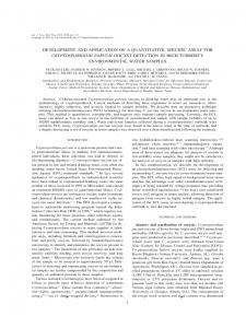
3. Application of Models-3/CMAQ-APT Figure 1. Interface between Models-3/CMAQ and SCICHEM. gas-phase formulation, i.e., aerosols and clouds were not treated. 2.3. Coupling of SCICHEM and Models-3/CMAQ [11] SCICHEM was imbedded into the host grid model following the established protocols for incorporating new science modules into Models-3/CMAQ. Figure 1 depicts the interactions between SCICHEM and the host model. SCICHEM is invoked in Models-3/CMAQ-APT by a single subroutine call similar to the invocation of any other physical or chemical process module in the host model. Like the other process modules in Models-3/CMAQ, all relevant information related to the emissions and the dynamic state of the atmosphere required by SCICHEM are accessed directly from the input files via the Input/ Output Applications Programming Interface (I/O API) [Coats et al., 1993]; only the three-dimensional concentration fields are shared directly between the host model and SCICHEM. On input to SCICHEM, these concentrations serve as the background (ambient) concentrations for SCICHEM calculations. On output from SCICHEM, these concentrations are updated whenever plume-to-grid transfer occurs and are returned to the host model. The transfer of puff material to the 3-D grid system (referred to as ‘‘puff dumping’’) occurs when the puff is determined to be chemically mature with respect to the host model. As an option, the model includes a physical criterion for dumping that is based on the horizontal size of the puff relative to the horizontal grid cell size. However, for fine grid resolutions, using a purely physical criterion may result in premature transfer of the plume material to the grid. As pointed out by Gillani and Pleim [1996], the chemical maturation of emissions from a large power plant is likely to take much longer than the time it takes for the plume to grow to the grid size for simulations with fine grids. Thus, it is appropriate to use the physical criterion option for coarse grid resolutions (e.g., several tens of kilometers) only. For the application presented here, we used the chemical criterion, described below. [12] The chemical criterion for maturity is based on the studies by Karamchandani et al. [1998], who defined three stages in the evolution of the chemistry of NOx plumes, and Gillani and Godowitch [1999], who used the plume concentration ratio of O3/Ox, where Ox = O3 + NO2, as a surrogate for the chemical age of the plume. A puff is assumed to be chemically mature whenever it is in the third stage of plume chemistry, as defined by Karamchandani et al. [1998], and

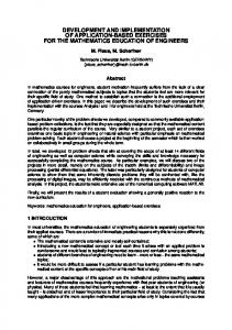
[13] The PiG model described above was applied to a domain covering the northeastern U.S., shown in Figure 2, for a five-day episode from 11 to 15 July 1995. The grid had a horizontal resolution of 12 km, while the vertical grid structure consisted of 13 layers from the surface to the tropopause with finer resolution near the surface (e.g., the surface layer is 18 m deep). The meteorological fields for the air quality modeling simulations were obtained from a prognostic simulation conducted with the nonhydrostatic meteorological model, MM5, using four-dimensional data assimilation (FDDA) [Seaman and Michelson, 2000]. [14] Figure 2 also shows the location of the thirty point sources with the highest NOx emission rates that were selected for explicit plume treatment in the Models-3/ CMAQ-APT simulation. These point sources represent 14% of the total NOx emission inventory over the coarse grid modeling domain. For convenience, we will refer to the Models-3/CMAQ-APT simulation as the ‘‘APT’’ simulation in the discussion that follows. [15] To determine the effect of using a PiG treatment, we conducted the following additional simulations: 1. A simulation with the base Models-3/CMAQ in which the thirty point sources referred to above were treated like

Figure 2. Modeling domain and locations of point sources with explicit plume-in-grid treatment.

ACH

12 - 4

KARAMCHANDANI ET AL.: STATE-OF-THE-SCIENCE PLUME-IN-GRID MODEL

Table 1. Model Performance Statistics for O3 Concentrations for 13 – 15 July 1995 Performance Statisticsa

Performance Measure

Models-3/CMAQ Base

Models-3/CMAQ-APT

1-hour Average O3 Concentrations 54% Paired peak errorb Gross error 29% Fractional gross error 0.28 Bias 12% Fractional bias 0.05

53% 29% 0.27 13% 0.06

8-hour Average O3 Concentrations 40% Paired peak errorb Gross error 25% Fractional gross error 0.23 Bias 11% Fractional bias 0.06

38% 25% 0.23 12% 0.07

a b

At 299 monitoring stations. Paired in both space and time.

the remaining point sources (i.e., without PiG treatment). We will refer to this simulation as the ‘‘Models-3/CMAQBase’’ or ‘‘Base’’ simulation. 2. A simulation with the base Models-3/CMAQ in which the emissions from the thirty point sources referred to above were excluded from the simulation. We will refer to this simulation as the ‘‘Models-3/CMAQ-Background’’ or ‘‘Background’’ simulation. [16] Before we investigate the effect of using a PiG treatment for the thirty point sources, it is useful to examine the performance of the model using surface O3 observations obtained from the U.S. EPA Aerometric Information Retrieval System (AIRS) database. There are approximately 300 AIRS monitoring sites in the modeling domain shown in Figure 2. In our evaluation of model performance, we compare model estimates of surface O3 concentrations from both the Base and APT simulations with corresponding observations. Because the first two days of the episode (11 and 12 July) were used to spin-up the model, results are presented for the last three days of the episode. 3.1. Evaluation of Model Performance [17] Table 1 shows the model performance statistics at 299 monitoring stations for the Base and APT simulations. The performance measures used are those defined by Seigneur et al. [2000] in their guidance document for the performance evaluation of three-dimensional grid models. The statistics were calculated for observed O3 concentrations greater than 40 ppb. Results are shown for both 1-hour and 8-hour average O3 concentrations. We see that the error for the peak O3 concentration paired in space and time is high for both the Base and APT simulations. The average gross error is less than 30% and the average bias is less than 15%. The overall model performance statistics for the Base and APT simulations are virtually identical. [18] The above results suggest that the overall model performance for surface O3 concentrations is not affected by using a PiG treatment. However, as shown in the following section, there are some significant differences in the surface O3 concentration predictions from the Base and APT simulations, particularly near the 30 point sources selected for PiG treatment in the APT simulation. The primary reason for the comparable model performance statistics

from the two simulations is that the differences between the simulations are minor or negligible at the majority of the AIRS monitoring stations in the modeling domain, since these stations are not influenced by the emissions from the 30 point sources. Furthermore, even at the monitoring sites where some differences are noted, the differences occur for only a few hours of the multiday episode. 3.2. Effect of Plume-in-Grid Treatment [19] We now examine the effect of using the PiG treatment for the 30 largest NOx point sources in the modeling domain on the modeled O3 and HNO3 surface concentrations. We present the results for O3 for two days (13 and 14 July) at the times of the maximum observed surface O3 concentration in the domain for each day (1500 EDT for both days). The results for surface HNO3 are presented for 13 July at 1500 EDT. The effects of the PiG treatment are shown as spatial plots of the differences in O3 and HNO3 surface concentrations between the APT and Base simulations. Therefore, a positive value means that the explicit treatment of point sources with the PiG model leads to a greater surface concentration of O3 or HNO3; a negative value means that the PiG treatment leads to a lower surface concentration. 3.2.1. Impact on Surface O3 Concentrations on 13 July and 14 July [20] Figure 3a shows the effect of the PiG treatment on modeled surface O3 concentrations at 1500 EDT on 13 July 1995. Several distinct patterns are seen in the figure. The patterns for some selected point sources and regions in the modeling domain are discussed below. 3.2.1.1. Southeastern U.S. [21] Most of the large NOx point sources selected for PiG treatment in this region are isolated sources that are located in an environment that is primarily NOx-limited for O3 formation. This pattern is best exemplified by the Belews Creek power plant located in Walnut Cove, North Carolina, because it is fairly well isolated from other point sources with PiG treatment. This source has the fifth highest NOx emissions of the 30 point sources selected for PiG treatment. [22] Figure 3a shows that, on 13 July, the North Carolina source plume travels to the north. The PiG treatment results in small increments in surface O3 concentrations (of the order of about 4 to 12 ppb) near and upwind of the source and large decrements in surface O3 concentrations (up to 32 ppb) from about 15 to 85 km immediately downwind (i.e., north of the source in Virginia) as compared to the Base simulation. [23] The near-source increment results from the fact that, in the APT simulation, the PiG treatment prevents the rapid mixing of the NOx emissions to the surface and, consequently, there is less titration of the existing O3 by the emitted NOx. In the Base simulation, the NOx emissions scavenge the surface O3 near and upwind of the source. The upwind transport of the point source emissions in the Base simulation is due to the numerical diffusion from the Bott [1989] advection scheme employed in the model. Such numerical artifacts have been noted in other applications of Bott’s scheme [e.g., Zhang et al., 1999]. As will be seen in the discussion that follows, this pattern of upwind transport of point source emissions in the Base simulation appears consistently for many of the point sources selected for PiG treatment in our study.

KARAMCHANDANI ET AL.: STATE-OF-THE-SCIENCE PLUME-IN-GRID MODEL

Figure 3. Differences in surface O3 concentrations between (a) APT and Base, (b) Base and Background, and (c) APT and Background simulations at 1500 EDT, 13 July 1995.

ACH

12 - 5

[24] The decrement in surface O3 concentrations further downwind is due to the faster production of surface O3 in the Base simulation than in the APT simulation. In the Base simulation, plume NOx is rapidly mixed within the grid system and to the surface and is therefore available for the production of O3 relatively quickly. In the APT simulation, the NOx emitted from the point source is mixed with the background air according to the rate of the plume dispersion and O3 formation is delayed until the plume has become sufficiently diluted. Thus, the PiG treatment reduces the formation of O3 from the point source NOx emissions by limiting the availability of the plume NOx. [25] Even further downwind, the O3 decrements become smaller, and the two simulations give identical results at about 170 km downwind. At downwind distances beyond 170 km, the surface O3 concentrations from the APT simulation are slightly higher (of the order of 2 to 3 ppb) than, or comparable to, those from the Base simulation. These small increments in surface O3 concentrations at very large downwind distances are due to differences in the VOC/NOx ratio in those grid cells between the APT and Base simulations. Since the PiG treatment will disperse the plume NOx more slowly, the NOx concentrations in the grid cells in the APT simulation will be greater than in the Base simulation once the plume size becomes commensurate with the grid cell size or the plume is chemically mature. Once O3 formation starts to take place in the plume, these higher NOx concentrations will slightly enhance O3 formation compared to the Base simulation if the background environment is NOx-limited. [26] The APT simulation also gives small O3 increments of about 2 to 8 ppb above the Base simulation at the eastern edge of the plume up to about 100 km from the source. These increments are due to the scavenging of surface O3 in the Base simulation by the NOx emitted from the source, as discussed later. [27] To better understand the above results, we now look at the Base and APT simulation results relative to the Background simulation results. Since the Background simulation was conducted without the 30 point sources, the differences between the Background simulation results and the APT and Base simulation results will show the effect of the NOx emissions from these point sources with and without PiG treatment, respectively. In other words, we can get a measure of the O3 (and HNO3) that can be produced (or sometimes destroyed, in the case of O3) in the plumes of these point sources with and without PiG treatment, particularly for isolated sources. [28] Figure 3b shows the difference between surface O3 concentrations from the Base and Background simulations at 1500 EDT on 13 July 1995. For many of the point sources, high O3 plumes are clearly visible with increments in downwind surface O3 concentrations of 30 to 40 ppb over the background value. Figure 3c shows the corresponding effect of the 30 point sources on O3 concentrations for the APT simulation. In contrast to the Base simulation, the downwind O3 increments at the surface are generally lower (of the order of 10 to 20 ppb) but spread over a larger region. The largest increments in surface O3 concentrations are of the order of 30 to 35 ppb and occur in the southwestern region of West Virginia. [29] Focussing on the isolated North Carolina point source, we see from Figure 3b that there is significant

ACH

12 - 6

KARAMCHANDANI ET AL.: STATE-OF-THE-SCIENCE PLUME-IN-GRID MODEL

Figure 4. Surface O3 concentrations downwind of the North Carolina point source at 1500 EDT, 13 July 1995. production of surface O3 downwind of this source when a PiG treatment is not used. The maximum increase in surface O3 concentration in the Base simulation is about 38 ppb over the Background simulation value of 84 ppb, and occurs due north of the source at a downwind distance of about 50 km. In contrast, as shown in Figure 3c, the maximum increase in surface O3 concentrations in the North Carolina point source plume in the APT simulation is about 12 ppb higher than the Background simulation value of 89 ppb at a location about 34 km northwest of the source. [30] Also, as discussed previously, we see from Figure 3b that, in the Base simulation, the North Carolina point source NOx emissions scavenge the surface O3 directly upwind (south) of the source and downwind along the eastern edge of the plume to a distance of about 100 km from the source. This results in small decrements in surface O3 concentrations of about 3 ppb south of the source and from 2 to 8 ppb on the eastern edge of the plume. In contrast, in the APT simulation, we see from Figure 3c that there is no scavenging of the surface O3 directly south of the source and along the eastern edge of the plume. However, increments in surface O3 concentrations of up to about 12 ppb occur to the southwest and northwest of the source. This increment corresponds to the maximum surface O3 produced in the APT simulation for this point source. Thus, it appears that, in the Base simulation, the plume travels primarily to the north, while in the APT simulation, there is some transport to the southwest and northwest of the source. An examination of the wind fields near the vicinity of the North Carolina point source in the hours leading up to 1500 EDT on 13 July reveals that there is a significant shift in wind direction between the lower and upper layers of the model. In the lower layers (up to about 1 or 1.5 km), the winds are primarily southerly, while in the upper layers the winds are northerly or northeasterly. In the Base simulation, the NOx emitted from the source is rapidly mixed down to the surface and the overall transport direction is primarily determined by the winds in the lower layers of the model. In the APT simulation, the vertical wind shear is resolved more accurately and the overall transport direction is also influenced by the upper layer winds. [31] The results for the North Carolina source show that, on 13 July, the increases in surface O3 concentrations due to its NOx emissions are much smaller when the PiG treatment

is used. The maximum surface O3 that can be attributed to the NOx emissions from the source in the APT simulation is about 26 ppb lower than that produced in the Base simulation on 13 July. This is further illustrated in Figure 4, which shows the surface O3 concentrations from the Background, Base, and APT simulations to the north of the North Carolina source at 1500 EDT on 13 July 1995. In the Base simulation, shown by the solid line, we note that rapid O3 production begins immediately downwind of the source. The difference between the surface O3 concentrations from the Base and Background simulations is about 21 ppb at about 17 km downwind from the source. The maximum increase, as noted previously, is about 38 ppb at 50 km downwind. Even at a downwind distance of 120 km, the surface O3 in the Base simulation is about 15 ppb higher than the background value. In contrast, in the APT simulation, the increase in surface O3 concentrations above the background value is about 5 ppb at 25 km from the source and grows to a maximum of about 10 ppb at a distance of about 80 to 100 km. [32] We also examine the plume surface O3 concentrations in more detail for some other selected sources in the southeastern U.S. for which it is easy to discern the effect of the PiG treatment. The TVA Cumberland power plant was the largest NOx emitter in the modeling domain for the period simulated. It is situated in a rural location in northern Tennessee, near the border with Kentucky, and approximately 80 km west of Nashville. The TVA Paradise power plant was the third largest NOx emitter and is located in Kentucky approximately 107 km NNE of the Cumberland power plant. [33] The results for the Cumberland and Paradise power plants are qualitatively similar to the results for the North Carolina point source. From Figures 3b and 3c, we see that, on 13 July, the Cumberland plume travels toward the NNE, and ultimately merges with the Paradise power plant plume. We also see that the APT simulation gives surface O3 concentrations that are significantly lower (by about 22 to 36 ppb) than the Base simulation downwind of the Cumberland power plant along the plume centerline. The APT simulation gives higher surface O3 concentrations (by about 7 to 18 ppb) than the Base simulation upwind of the source and along the western edge of the plume. [34] Figure 3b shows that, in the Base simulation, there is initial scavenging of the background surface O3 of about 4 ppb upwind of the Cumberland power plant and of up to about 5 ppb along the western edge of the plume. However, rapid O3 production begins immediately downwind of the source. The peak surface O3 production downwind of Cumberland in the Base simulation is about 41 ppb over the background value of 96 ppb and occurs at about 43 km northeast of the power plant. In contrast, the peak surface O3 production in the Cumberland plume in the APT simulation occurs further downwind at about 70 km north of the power plant and is about 17 ppb over the background value of about 102 ppb (Figure 3c). [35] Similarly, Figure 3a shows that the downwind surface O3 concentrations from the APT simulation in the combined Cumberland-Paradise plume are significantly lower (by as much as 32 ppb) than the corresponding Base simulation concentrations on 13 July. The maximum downwind surface O3 production in the Base simulation in the combined plume is about 43 ppb over the background value of about 94 ppb (Figure 3b) and occurs northeast of the

KARAMCHANDANI ET AL.: STATE-OF-THE-SCIENCE PLUME-IN-GRID MODEL

Paradise power plant at a distance of about 43 km from the plant. This is also the location of the maximum downwind surface O3 production in the APT simulation, about 12 ppb higher than the background value (Figure 3c). 3.2.1.2. Midwestern U.S. [36] This region includes some large isolated NOx point sources in rural areas, as well as two point sources in northeastern Illinois to the southwest of Chicago, and two point sources in eastern Michigan. We first briefly discuss the results of the PiG treatment for the two point sources in southwestern and south-central Illinois, and the point source in north-central Illinois. The results for these sources are qualitatively similar to those discussed above for the southeastern U.S. The plumes from these sources travel toward the northeast on 13 July. The plume from the southwestern Illinois source eventually merges with that from the south-central Illinois source. The maximum surface O3 produced in the Base simulation in the plume is about 38 ppb over the background value of 93 ppb (Figure 3b), at approximately 27 km northeast of the source. The maximum surface O3 produced in the APT simulation is about 18 ppb over the background value of 109 ppb (Figure 3c), and occurs to the northeast of the source at a much larger distance (approximately 94 km) than the Base simulation maximum. Similarly, the Base simulation gives a maximum surface O 3 production northeast from the south-central Illinois point source of 23 ppb above the background value of 127 ppb, at a distance of approximately 34 km. The corresponding maximum surface O3 production from the south-central Illinois source in the APT simulation also occurs northeast of the source, but at a larger downwind distance of approximately 85 km (Figure 3c). The APT surface O3 concentration at this location is 120 ppb, 19 ppb above the background value. [37] For the north-central Illinois point source, the maximum increase in surface O3 concentrations over the background values in the Base simulation is about 24 ppb on 13 July, and occurs northeast of the source at a distance of approximately 70 km (Figure 3b). Figure 3c shows that the maximum surface O3 produced in the APT simulation from this source occurs to the NNE at a much larger downwind distance (approximately 160 km). The surface O3 concentration from the APT simulation at this location is about 106 ppb, about 18 ppb over the background value. Also note that some of the emissions from this source are transported north into Wisconsin in the Base simulation, leading to surface O3 formation of 5 to 15 ppb above the background value in northern Illinois and southern Wisconsin (Figure 3b). On the other hand, Figure 3c shows that there is little transport in this direction in the APT simulation. Thus, the O3 concentrations from the APT simulation in northern Illinois and southern Wisconsin are comparable to the background value, resulting in the APT simulation giving lower O3 concentrations in the region compared to the Base simulation (Figure 3a). [38] Somewhat different patterns are seen in the comparison of the APT and Base simulations for the two large NOx point sources in northeastern Illinois, possibly due to differences in the VOC/NOx ratios as well as to differences in the meteorology. For example, although the eastern U.S. is primarily NOx-limited with respect to O3 formation during summertime [Jacob et al., 1995], some urban areas such as

ACH

12 - 7

Chicago, Illinois are VOC-limited [e.g., Blanchard et al., 1999; Sillman, 1999; Blanchard, 2000] (B. K. Pun et al., Day of the week behavior of atmospheric ozone in three United States cities, submitted to Environmental Science and Technology, 2002). On 13 July, the plumes of the two point sources located in northeastern Illinois are transported over the Chicago area. Since the background environment is VOC-limited, the effect of the PiG treatment is primarily to limit titration of O3 by NO and we see from Figure 3a that the APT simulation results in higher surface O3 concentrations than the Base simulation over the Chicago area and over the southern part of Lake Michigan. This is confirmed by Figures 3b and 3c, which show that the surface O3 concentrations downwind of the two northeastern Illinois point sources in the Base simulation are up to 17 ppb lower than the background value, while the APT simulation surface O3 concentrations are the same as or within 5 ppb of the background values. [39] The patterns for the two point sources in eastern Michigan, one on the shore of Lake Huron at Saginaw Bay and the other to the southeast near Detroit, are similar to those for the point sources upwind of Chicago. Figure 3a indicates that the APT simulation gives much larger surface O3 concentrations (up to about 60 ppb) than the Base simulation downwind (northeast) of the Saginaw Bay point source. However, as Figures 3b and 3c show, this increase is a direct result of the relatively larger titration of surface O3 concentrations by the NOx emissions from the point source in the Base simulation as compared to the APT simulation. In the Base simulation, as much as 69 ppb of the background surface O3 concentration of approximately 107 ppb are titrated, while the maximum titration of background surface O3 in the APT simulation is only about 20 ppb. 3.2.1.3. The Ohio River Valley [40] The patterns observed near the Ohio River Valley and in its downwind areas are more complex because of the large number of point sources with explicit plume-in-grid treatment (9 point sources along the borders of Ohio, Kentucky and West Virginia; see Figure 2) and the complex wind flow patterns around the Appalachian Mountains. Thus, some point source plumes are transported north and northeast over Ohio and Pennsylvania whereas other point source plumes are transported south and east over the Appalachian Mountains into West Virginia. The effect of the PiG treatment on downwind O3 concentrations is a complex mixture of O3 decrements and increments between the APT and Base simulations. [41] On 13 July, we see from Figure 3a that the APT simulation gives lower surface O3 concentrations than the Base simulation north of the two point sources in southern Ohio, one located along the border with Kentucky, and the other located along the border with West Virginia. On the other hand, the APT simulation gives higher surface O3 concentrations than the Base simulation in most of West Virginia as well as over western and northern Pennsylvania northeast of the Ohio River Valley. To understand the reasons for these differences, we again refer to Figures 3b and 3c, which show the changes in surface O3 concentrations from the Base and APT simulations, respectively, relative to the Background simulation. The decrements (in the APT simulation with respect to the Base simulation) in central and northern Ohio, as well as in the western portion

ACH

12 - 8

KARAMCHANDANI ET AL.: STATE-OF-THE-SCIENCE PLUME-IN-GRID MODEL

of West Virginia (immediately to the east and southeast of the point sources in southeastern Ohio and West Virginia) are associated with higher production of surface O3 in the Base simulation than in the APT simulation. On the other hand, the increments in western and northern Pennsylvania are primarily associated with larger titration of surface O3 by the NOx emitted from the Ohio River Valley sources in the Base simulation as compared to the APT simulation, rather than with higher O3 production in the APT simulation compared to the Base simulation. These results are qualitatively similar to the results for the other point sources discussed so far and for most of the point sources selected for PiG treatment in our study. [42] In contrast, the increments in the central portion of West Virginia are associated with increased production of O3 in the APT simulation as compared to the Base simulation. The NOx emissions from the sources in southeastern Ohio and in West Virginia undergo rapid mixing as they are transported over complex terrain into West Virginia. In the Base simulation, this results in enhanced production of both surface HNO3 (see section 3.2.3) and some O3 immediately downwind of the sources, leading to a depletion of NOx in the plumes, and a consequent reduction in surface O3 production, by the time they arrive in central West Virginia. In the APT simulation, the production of both surface HNO3 and O3 also begins occurring immediately downwind but at a slower rate than in the Base simulation, resulting in the peak production occurring later downwind, when the plumes reach central West Virginia. [43] The results for 14 July are generally similar to those for 13 July. However, there are some important differences, and we focus our attention on these differences in the discussion below. [44] Figure 5a shows the difference in surface O3 concentrations between the APT and Base simulations on 14 July, at 1500 EDT. Figures 5b and 5c show the surface O3 concentration differences relative to the background values for the Base and APT simulations, respectively. [45] The results for the two point sources located in northeastern Illinois show some important differences from the 13 July results. Recall from our earlier discussion that, on 13 July, the plumes from these sources were transported to the northeast, over the VOC-limited Chicago area and over the southern part of Lake Michigan. However, on 14 July, Figures 5a through 5c show that these plumes are transported eastward toward Indiana, into an environment that is likely to be NOx-limited. The 13 July results showed that in the Base simulation, the NOx emissions from the two sources titrated the background surface O3 to large downwind distances, while in the APT simulation, the NOx emissions were transported aloft, resulting in downwind surface O3 concentrations that were comparable to the background values. Thus, the APT simulation gave higher surface O3 concentrations downwind of the sources than the Base simulation. For both simulations, there was negligible surface O3 production downwind of the sources on 13 July. On the other hand, we see from Figure 5b that, in the Base simulation on 14 July, there is some initial titration of background surface O3, followed by some production of O3 in the plumes from these sources. In contrast, the downwind surface O3 concentrations from the APT simulation on 14 July are comparable to the background values. This results in the APT simulation giving

Figure 5. Differences in surface O3 concentrations between (a) APT and Base, (b) Base and Background, and (c) APT and Background simulations at 1500 EDT, 14 July 1995.

KARAMCHANDANI ET AL.: STATE-OF-THE-SCIENCE PLUME-IN-GRID MODEL

lower surface O3 concentrations downwind of the sources than the Base simulation. [46] As on 13 July, we note some complex patterns near the Ohio River Valley and in its downwind areas on 14 July. While the overall results for 14 July for this region are qualitatively similar to those for 13 July, the results for Pennsylvania show some differences. Figure 5b shows that the transport of the Ohio River Valley emissions to the northeast into Pennsylvania results in increases of surface O3 concentrations of up to 35 ppb over background values on 14 July in the Base simulation. Figure 5c shows that O3 is also produced in the APT simulation as the Ohio River Valley emissions are transported into Pennsylvania, but in lower amounts than in the Base simulation. Thus, the comparison between the APT and Base simulations shows decrements on 14 July in the western half of Pennsylvania (Figure 5a). In contrast, the results for 13 July showed that in the Base simulation, the NOx emitted from the Ohio River Valley sources resulted in titration of surface O3 in western and northern Pennsylvania (Figure 3b) leading to higher surface O3 concentrations in this region in the APT simulation than in the Base simulation (Figure 3a). We also note that, in the APT simulation for 14 July, the maximum increase in downwind surface O3 concentrations in West Virginia due to the NOx emissions from the Ohio River Valley sources is more than 80 ppb, much larger than the maximum increase on 13 July (36 ppb). [47] The results presented here show that the maximum surface O3 concentrations downwind of major NOx point sources are generally in excess of the background values by about 30 to 40 ppb in the Base simulation and by about 10 to 20 ppb in the PiG simulation at 1500 EDT on 13 and 14 July 1995. The notable exception to this generalization is in West Virginia, downwind of the Ohio River Valley sources, where the APT simulation produces larger downwind surface O3 concentrations over background values than the Base simulation. [48] It is interesting to compare these results with those from power plant plume measurements. For example, several measurements of the Cumberland power plant plume were conducted by instrumented aircraft during the 1995 SOS-Nashville Field Study [Gillani et al., 1998]. Some of these measurements were conducted in July, the same month as simulated in this study, although the measurement days (7, 16, 17, and 19 July) do not coincide with our simulation period. The local instantaneous maximum O3 concentrations in the plume exceeded background O3 values by about 20 ppb on 7 July to about 50 ppb on 16 July [Gillani et al., 1998]. While these increments are larger than the APT simulation results presented in Figures 3c and 5c, it is important to note the following inconsistencies in the comparison between simulated and measured O3 increments: 1. The Cumberland plume measurements were conducted at plume height (ranging from 300 to 1400 m MSL) while the model results shown here are surface (first model layer) values 2. The Cumberland plume measurements were conducted at various times of the day, while the model results are presented for 1500 EDT 3. The measured O3 increments in the Cumberland plume pertain to local instantaneous maximum values, while the model results are hourly grid-cell averaged values

ACH

12 - 9

4. The measurement days do not coincide with the simulation days [49] While it is not feasible to account for the last two inconsistencies listed above, we can attempt to account for the first two inconsistencies by determining the O3 increments (over background values) downwind of Cumberland in the upper layers of the model for all the daylight hours. On 13 July, the maximum O3 increment in the Cumberland plume was about 52 ppb for the APT simulation at 1900 EDT in the 8th model layer (i.e., between 1 and 1.5 km) and a downwind distance of about 50 km. On 14 July, the maximum increment was about 38 ppb at 1700 EDT and a downwind distance of about 60 km, also in the 8th model layer. The maximum O3 increment on 15 July was about 43 ppb at 1900 EDT in the 8th model layer at a downwind distance of about 100 km. These plume increments are comparable with those measured during the 1995 SOSNashville Field Study [Gillani et al., 1998]. In comparison, the maximum increments in downwind surface O3 concentrations in the APT simulation ranged from 26 ppb at 1800 EDT on 13 July to 36 ppb at 1900 EDT on 15 July. [50] We also determined the O3 increments downwind of Cumberland in the upper layers and all daylight hours for the Base simulation. In general, the vertical profile of O3 increments is more uniform in the Base simulation than in the APT simulation. For example, on 13 and 14 July, the O3 increment from the Base simulation varies from about 40 ppb at 1500 EDT to about 50 ppb at 2000 EDT in the first 8 layers of the model. The maximum increment of 51 ppb on 13 July occurs in layers 4 through 6 (i.e., 100 to 750 m) at 2000 EDT at a downwind distance of about 50 km. The maximum increment of 55 ppb on 14 July occurs in layer 4 (i.e., 100 to 250 m) at 2000 EDT at a downwind distance of about 24 km. On 15 July, the O3 increment from the Base simulation is of the order of 50 ppb from 1800 to 2000 EDT in the first 8 layers of the model, with the maximum increment of 55 ppb occurring in layers 4 through 8 (i.e., 100 to 1500 m) at 2000 EDT and a downwind distance of about 100 km. 3.2.2. Impact on HNO3 Concentrations on 13 July [51] Spatial patterns of surface HNO3 concentration differences between the APT and Base simulations are shown in Figure 6a at 1500 EDT on 13 July. The patterns for the HNO3 concentration differences show some similarities with those obtained for the O 3 concentration differences. However, there are also some differences, as discussed below. [52] The surface HNO3 results for the isolated North Carolina source, the Cumberland and Paradise power plants, and the point sources located in southern and central Illinois are qualitatively similar to the surface O3 results discussed earlier. For all these sources, the APT simulation gives lower surface HNO3 concentrations than the Base simulation immediately downwind of the sources, but gives higher concentrations at the plume edges and further downwind of the sources. As in the discussion of the O3 results, we use the Background simulation to determine the extent of HNO3 formation in the plumes with and without PiG treatment. Figures 6b and 6c present the differences in surface HNO3 concentrations between the Base and Background simulations and between the APT and Background simulations, respectively, for 13 July.

ACH

12 - 10

KARAMCHANDANI ET AL.: STATE-OF-THE-SCIENCE PLUME-IN-GRID MODEL

Figure 6. Differences in surface HNO3 concentrations between (a) APT and Base, (b) Base and Background, and (c) APT and Background simulations at 1500 EDT, 13 July 1995.

[53] Figure 6b shows that, downwind of the North Carolina point source, nearly 10 ppb of surface HNO3 is produced (above the background value) in the Base simulation. However, upwind of the source and along the eastern edge of the plume, where the plume NOx scavenges the background O3 (see Figure 3b), we see that the effects of the point source emissions are small reductions in surface HNO3 concentrations when a PiG treatment is not used. In contrast, Figure 6c shows that, when a PiG treatment is used, small amounts of surface HNO3 (generally less than 2 ppb) are formed in the plume up to about 220 km downwind of the source. [54] In the Cumberland plume, a maximum of about 6 ppb of surface HNO3 is formed in the Base simulation over the background value of 4 ppb. In the APT simulation, the maximum surface HNO3 produced is less than 4 ppb over a background value of 4 ppb. Similarly, the maximum surface HNO3 produced downwind of the southern Illinois source in the Base simulation is nearly 7 ppb over the background value of 8 ppb, while the maximum HNO3 produced in the APT simulation is slightly more than 4 ppb over the background value of 7 ppb. [55] Some differences between the surface O3 and HNO3 patterns are apparent in the results for the eastern Michigan point source located near Saginaw Bay and for the regions downwind of the Ohio River Valley for 13 July. Figure 6b shows that there is initial depletion, followed by some formation of surface HNO3 in the plume (up to about 5 ppb over the background value of 13 ppb) downwind of the Saginaw Bay point source in the Base simulation. In the APT simulation, small amounts of surface HNO3 are produced downwind of the source (the maximum production is about 2 ppb over a background value of about 23 ppb), as shown in Figure 6c. However, as discussed earlier, large reductions in background O3 concentrations (see Figure 3b) are obtained downwind of the source due to titration by the NOx in the plume in the Base simulation, while the corresponding reductions in the APT simulation (Figure 3c) are much smaller. Thus, the downwind O3 concentrations in the APT simulation are higher than those in the Base simulation (because less background O3 is titrated with PiG treatment), but the downwind HNO3 concentrations in the APT simulation are lower than the Base simulation (because less HNO3 is produced with PiG treatment). [56] Also, we see from Figure 6a that the HNO3 concentrations from the APT simulation in the region around the Ohio River Valley are significantly lower than the Base simulation values on 13 July, except over the central portion of West Virginia. For the O3 concentrations we had noted an increase in O3 concentrations over most of West Virginia in the APT simulation as compared to the Base simulation (note, however, that the HNO3 and O3 increments between the APT and Base simulations over the central portion of West Virginia are qualitatively similar). [57] To understand the similarities and differences in the O3 and HNO3 patterns discussed above, it is useful to briefly review the chemistry of HNO3 and O3 formation in NOx plumes. In a plume rich in NOx, oxidants are depleted initially and formation of oxidation products such as HNO3 and H2SO4 is suppressed. As the plume becomes more dilute, these oxidation products will start to form, albeit at a

KARAMCHANDANI ET AL.: STATE-OF-THE-SCIENCE PLUME-IN-GRID MODEL

rate slower than the rate in the background air (i.e., outside the plume). Further downwind, in a NOx-limited environment, the formation of oxidants such as O3 may exceed that of the background. The formation rate of HNO3 farther downwind in the plume will differ depending on whether the background is NOx- or VOC-limited [Karamchandani and Seigneur, 1999]. In a VOC-limited environment, the HNO3 plume concentration will increase steadily as the VOC/NOx ratio approaches that of the background. In a NOx-limited environment, the HNO3 formation rate will increase rapidly as the VOC-limited plume environment is more conducive to HNO3 formation than the background; as the plume becomes more dilute, the HNO3 formation rate will decrease toward that of the background. Although O3 and HNO3 concentrations in a plume follow similar trends as the plume becomes dispersed, it is important to note that in a NOx-limited environment, HNO3 formation occurs earlier than O3 formation in the plume and, further downwind, plume HNO3 concentrations decrease more rapidly than plume O3 concentrations. [58] Thus, in the Base simulation, we note from Figure 6b that a significant amount of surface HNO3 is produced in the western portion of West Virginia near the border with Ohio due to the emissions from the point sources located in southeastern Ohio and in West Virginia. The maximum surface HNO3 produced is about 27 ppb (over a background value of only 6 ppb) in the grid cell immediately to the northeast of the West Virginia point source. At this location, the surface HNO3 production in the APT simulation is only about 5 ppb over the background value. Further downwind, the production of surface HNO3 in the Base simulation decreases, but production in the APT simulation continues. 3.2.3. Impact on O3 and HNO3 Mass Budgets [59] Over the five-day simulation period, the total O3 mass integrated across the modeling domain over all model layers is slightly higher (0.2%) in the APT simulation than in the Base simulation. In the surface layer, the total O3 mass integrated across the modeling domain is also slightly higher (0.6%) in the APT simulation than in the Base simulation. This result, and the results presented earlier in this section, indicate that the generally lower production of O3 downwind of major NOx point sources in the APT simulation is more or less compensated by the unrealistically large titration of existing surface O3 by the NOx emissions in the Base simulation without PiG treatment. [60] Over the five-day period and the entire modeling domain, the APT simulation leads to 3% less HNO3 than the Base simulation. In the surface layer, the APT simulation leads to 6% less HNO3 than the Base simulation. This difference is primarily due to the generally lower production of HNO3 downwind of the major NOx point sources in the APT simulation as compared to the Base simulation.

4. Summary and Conclusions [61] A new state-of-the science plume-in-grid model, Models-3/CMAQ-APT, has been developed and applied to the Northeastern United States, using a horizontal grid resolution of 12 km, for a five-day O3 episode in July 1995. The thirty largest NOx point sources in the modeling domain were explicitly simulated with PiG treatment. To

ACH

12 - 11

determine the effects of the PiG treatment, two additional simulations were conducted. In the first simulation, referred to as the ‘‘Base’’ simulation, all point sources, including the 30 largest NOx point sources, were treated in the host grid model, i.e., without a PiG treatment. In the second simulation, referred to as the ‘‘Background’’ simulation, emissions from the 30 largest NOx point sources were neglected. Differences in the results between the Background simulation and the Base and APT simulations provide a measure of the contribution of these point sources to surface O3 and HNO3 concentrations with and without PiG treatment. [62] The simulation results show that the use of Models3/CMAQ-APT has a significant effect on the spatial patterns of O3 and HNO3 surface concentrations downwind of the sources considered for PiG treatment to distances of 100 to 200 km. Surface O3 concentrations from the APT simulation show both decrements and increments with respect to the Base simulation. The maximum decrement is about 80 ppb, and the maximum increment is about 77 ppb. The decrements and increments compensate each other so that over the entire domain and episode, the difference between the total O3 mass in the two simulations is negligible (0.2%). [63] A comparison of the Base simulation and APT simulation results with those from the Background simulation shows that most of the surface O3 decrements are associated with lower production of O3 immediately downwind of the point sources in the APT simulation relative to the Base simulation. For a majority of the point sources considered for PiG treatment in the simulation, the maximum increases in surface O3 concentrations in the Base simulation over the Background simulation values are generally 5 to 30 ppb higher than the corresponding increases in the APT simulation. Furthermore, O3 production is generally delayed in the APT simulation as compared to the Base simulation. In the Base simulation, the maximum increases in surface O3 concentrations over the background values generally occur within downwind distances of about 50 km, while in the APT simulation, the maximum increases typically occur further downwind, at distances of 100 to 200 km. [64] With one exception, the large increments in surface O3 concentrations between the APT and Base simulations are primarily associated with the higher titration of background surface O3 in the Base simulation near and upwind of the point sources, particularly in VOC-limited environments. When the PiG treatment is used, the plume NO remains aloft and is not available for titrating surface O3 concentrations near the source. An exception to the above generalization occurs in West Virginia, downwind of the Ohio River Valley point sources. Large increments in surface O3 concentrations between the APT and Base simulations are noted, particularly on 14 July, that are primarily associated with higher O3 production further downwind in the APT simulation than in the Base simulation. In the Base simulation, the NOx in the plume undergoes rapid conversion to HNO3 and O3 within 25 to 50 km of the sources, leading to a depletion of NOx, and a consequent reduction in O3 production, at larger downwind distances. In the APT simulation, the conversion of NOx to HNO3 occurs at a slower rate, so that more NOx is available for O3 production

ACH

12 - 12

KARAMCHANDANI ET AL.: STATE-OF-THE-SCIENCE PLUME-IN-GRID MODEL

at larger downwind distances (about 150 to 200 km from the sources in southeastern Ohio). Note that the combined NOx emissions from the cluster of sources in southeastern Ohio and West Virginia are almost three times higher than that from the single largest source in the modeling domain (the Cumberland power plant). [65] The smaller increments (typically less than 10 ppb) between the APT and Base simulations are associated with both higher titration of existing surface O3 in the Base simulation and delayed production of O3 further downwind in the APT simulation, as the plume NOx is transported and exposed to a NOx-limited environment. [66] While the surface O3 increments (relative to background values) downwind of major NOx point sources are generally below 30 ppb in the PiG simulation, the increments in the upper model layers are of the order of 30 to 50 ppb, comparable with those measured in power plant plumes. [67] For surface HNO3 concentrations, the differences between the APT and Base simulations range from a maximum decrement of 24 ppb to a maximum increment of 9 ppb. The APT simulation generally gives lower surface HNO3 concentrations than the Base simulation over a large portion of the modeling domain. Over the entire domain and episode, the PiG treatment leads to a decrease in HNO3 mass of 3%. [68] The overall model performance statistics for 1-hour and 8-hour averaged surface O3 concentrations from the Base and PiG simulations are almost identical despite the differences noted above. While the PiG simulation results are more consistent with our understanding of power plant plume chemistry than the Base simulation results, a more rigorous testing of the model would require a comparison of the results with those from fine grid simulations as well as other techniques used to resolve subgrid-scale features, such as interactive static nested grids, or adaptive grid algorithms. Note that for such a comparison (e.g., a coarse grid simulation with PiG treatment for major point sources versus a fine grid simulation without PiG treatment) to be valid, it would be necessary to ensure that only the alternative techniques for resolving point sources are compared. In other words, the effects of other subgrid-scale features (e.g., subgrid-scale variations in terrain, meteorology, and surface emissions) should be eliminated by using the coarse grid fields for the fine grid simulation. [69] The results from this study suggest that it is desirable to use a PiG treatment for major NOx point sources, since both surface O3 and HNO3 production downwind of these sources are generally overpredicted if a PiG treatment is not used. [70] Acknowledgments. This work was conducted under funding from EPRI Project EP-P2543/C1152. Thanks are due to the EPRI Project Managers, Naresh Kumar and Alan Hansen, for their support. We would like to acknowledge the contributions of Ian Sykes and Lynne Santos (presently with ENSR International) of Titan, Inc., who led the development of the reactive plume model, SCICHEM, used in Models-3/CMAQAPT. We also thank the Coordinating Research Council (CRC) for allowing us to use the CRC Project A-23 meteorological and emission input files for the NARSTO-Northeast modeling domain. We are grateful to the Division of Air Resources at the New York State Department of Environmental Conservation (NYSDEC) for providing surface ozone concentrations from the Aerometric Information Retrieval System (AIRS) database for evaluating the models used in this work. Finally, we are grateful to the JGR

reviewers for their useful suggestions on the improvement of this manuscript.

References Blanchard, C. L., Ozone process insights from field experiments, 3, Extent of reaction and ozone formation, Atmos. Environ., 34, 2035 – 2043, 2000. Blanchard, C. L., F. W. Lurmann, P. M. Roth, H. E. Jeffries, and M. Korc, The use of ambient data to corroborate analyses of ozone control strategies, Atmos. Environ., 33, 369 – 381, 1999. Bott, A., A positive definite advection scheme obtained by nonlinear renormalization of the advection fluxes, Mon. Weather Rev., 117, 1006 – 1115, 1989. Byun, D. W., and J. K. S. Ching, Science algorithms of the EPA Models-3 Community Multiscale Air Quality (CMAQ) modeling system, EPA-600/ R-99/030, U.S. Environmental Protection Agency, Washington, D. C., 1999. Coats, C. J., A. Hanna, D. Hwang, and D. W. Byun, Model engineering concepts for air quality models in an integrated environmental modeling system, paper presented at AWMA Specialty Conference on Regional Photochemical Measurement and Modeling Studies, San Diego, Calif., 8 – 12 November 1993. Gillani, N. V., Ozone formation in pollutant plumes: Development and application of a reactive plume model with arbitrary crosswind resolution, EPA-600/S3-86-051, U.S. Environmental Protection Agency, Research Triangle Park, N. C., 1986. Gillani, N. V., and J. M. Godowitch, Plume-in-grid treatment of major point source emissions, in Science Algorithms of the EPA Models-3 Community Multiscale Air Quality (CMAQ) Modeling System, chapter 9, 9-1 – 9-39, EPA-600/R-99/030, U.S. Environmental Protection Agency, Washington, D. C., 1999. Gillani, N. V., and J. E. Pleim, Subgrid scale features of anthropogenic emissions of NOx and VOC in the context of regional Eulerian models, Atmos. Environ., 30, 2043 – 2059, 1996. Gillani, N. V., J. F. Meagher, R. J. Valente, R. E. Imhoff, R. L. Tanner, and M. Luria, Relative production of ozone and nitrates in urban and rural power plant plumes, 1, Composite results based on data from 10 field measurements days, J. Geophys. Res., 103, 22,593 – 22,615, 1998. Jacob, D. J., L. W. Horowitz, J. W. Munger, B. G. Heikes, R. R. Dickerson, R. S. Artz, and W. C. Keene, Seasonal transition from NOx- to hydrocarbon-limited conditions for ozone production over the eastern United States, J. Geophys. Res., 100, 9315 – 9324, 1995. Karamchandani, P., and C. Seigneur, Simulation of sulfate and nitrate chemistry in power plant plumes, J. Air Waste Manage. Assoc., 49, 175 – 181, 1999. Karamchandani, P., A. Koo, and C. Seigneur, A reduced gas-phase kinetic mechanism for atmospheric plume chemistry, Environ. Sci. Technol., 32, 1709 – 1720, 1998. Karamchandani, P., L. Santos, I. Sykes, Y. Zhang, C. Tonne, and C. Seigneur, Development and evaluation of a state-of-the-science reactive plume model, Environ. Sci. Technol., 34, 870 – 880, 2000. Kumar, N., and A. G. Russell, Multiscale air quality modeling of the northeastern United States, Atmos. Environ., 30, 1099 – 1116, 1996a. Kumar, N., and A. G. Russell, Development of a computationally efficient, reactive subgrid-scale plume model and the impact in the northeastern United States using increasing levels of chemical detail, J. Geophys. Res., 101, 16,737 – 16,744, 1996b. Kumar, N., M. T. Odman, and A. G. Russell, Multiscale air quality modeling: Application to southern California, J. Geophys. Res., 99, 5385 – 5397, 1994. Morris, R. E., M. A. Yocke, T. C. Myers, and R. C. Kessler, Development and testing of UAM-V: A nested-grid version of the Urban Airshed Model, paper presented at AWMA Specialty Conference on Tropospheric Ozone and the Environment II, Atlanta, Georgia, 4 – 7 November 1991. Myers, T. C., P. D. Guthrie, and S.-Y. Wu, The implementation of a plumein-grid module in the SARMAP Air Quality Model (SAQM), SYSAPP96/06, Systems Applications International, Inc., San Rafael, Calif., 1996. Odman, M. T., and A. G. Russell, Multiscale modeling of pollutant transport and chemistry, J. Geophys. Res., 96, 7363 – 7370, 1991. Richards, L. W., J. A. Anderson, D. L. Blumenthal, A. Brandt, J. A. McDonald, N. Waters, E. S. Macias, and P. S. Bhardwaja, The chemistry, aerosol physics and optical properties of a western coal-fired power plant plume, Atmos. Environ., 15, 2111 – 2134, 1981. Seaman, N. L., and S. A. Michelson, Mesoscale meteorological structure of a high-ozone episode during the 1995 NARSTO-Northeast Study, J. Appl. Meteorol., 39, 384 – 398, 2000. Seigneur, C., T. W. Tesche, P. M. Roth, and M. K. Liu, On the treatment of point source emissions in urban air quality modeling, Atmos. Environ., 17, 1655 – 1676, 1983. Seigneur, C., et al., Guidance for the performance evaluation of three-di-

KARAMCHANDANI ET AL.: STATE-OF-THE-SCIENCE PLUME-IN-GRID MODEL mensional air quality modeling systems for particulate matter and visibility, J. Air Waste Manage. Assoc., 50, 588 – 599, 2000. Sillman, S., The relation between ozone, NOx and hydrocarbons in urban and polluted rural environments, Atmos. Environ., 33, 1821 – 1845, 1999. Sillman, S., J. A. Logan, and S. C. Wofsy, A regional scale model for ozone in the United States with subgrid representation of urban and power plant plumes, J. Geophys. Res., 95, 5731 – 5748, 1990. Srivastava, R. K., D. S. McRae, and M. T. Odman, Simulation of dispersion of a power plant plume using an adaptive grid algorithm, Atmos. Environ., 35, 4801 – 4818, 2001. Sykes, R. I., and D. S. Henn, Representation of velocity gradient effects in a Gaussian puff model, J. Appl. Meteorol., 34, 2715 – 2723, 1995. Sykes, R. I., W. S. Lewellen, S. F. Parker, and D. S. Henn, A hierarchy of dynamic plume models incorporating uncertainty, vol. 4, Second-order closure integrated puff, EPRI EA-6095, vol. 4, Project 1616-28, EPRI, Palo Alto, Calif., 1988.

ACH

12 - 13

Sykes, R. I., S. F. Parker, D. S. Henn, and W. S. Lewellen, Numerical simulation of ANATEX tracer data using a turbulence closure model for long-range dispersion, J. Appl. Meteorol., 32, 929 – 947, 1993. Tomlin, A., M. Berzins, J. Ware, J. Smith, and M. J. Pilling, On the use of adaptive gridding methods for modelling chemical transport from multiscale sources, Atmos. Environ., 31, 2945 – 2959, 1997. Zhang, Y., C. Seigneur, J. H. Seinfeld, M. Z. Jacobson, and F. S. Binkowski, Simulation of aerosol dynamics: A comparative review of algorithms used in air quality models, Aerosol Sci. Technol., 31, 487 – 514, 1999.

P. Karamchandani, C. Seigneur, K. Vijayaraghavan, and S.-Y. Wu, Atmospheric and Environmental Research, Inc., 2682 Bishop Drive, Suite 120, San Ramon, CA 94583, USA. ( [email protected])