DISSIPATIVE PARTICLE DYNAMICS AND OTHER FLUID PARTICLE

Chapter 1 DISSIPATIVE PARTICLE DYNAMICS AND OTHER FLUID PARTICLE MODELS Pep Espa˜ nol Abstract

1.

Dissipative Particle Dynamics is a particle model that allows to simulate complex fluids at mesoscopic scales. Since its introduction a decade ago it has been applied to a large variety of different complex fluid systems. At the same time, generalizations of the model have been introduced in order to refine the concept of dissipative particle. Here, I offer my personal view about the status of DPD as a model for simulating complex fluids, review part of the literature on applications, and sketch some lines for future research.

Introduction

The Dissipative Particle Dynamics model was initially devised by Hoogerbrugge and Koelman as a simulation method to avoid the lattice artifacts of Lattice Gas Automata and yet capturing hydrodynamic time and space scales much larger than those available with Molecular Dynamics [1]. The DPD model consists on a set of point particles that move off-lattice interacting with each other through a set of prescribed forces [1, 2]. These forces are of three types: a purely repulsive conservative force, a dissipative force that tries to reduce velocity differences between the particles, and a further stochastic force directed along the line joining the center of the particles. The amplitude of these forces is dictated by a Fluctuation-Dissipation theorem [2]. The forces are modulated with a weight function (usually a Mexican hat function) that specifies the range of interaction between dissipative particles and renders this interaction local. The distinguishing feature of the DPD forces is that they conserve momentum and, therefore, the DPD model captures the essentials of mass and momentum conservation which are the responsible for the hydrodynamic behaviour of a fluid at large scales [3, 4].

1

2 From a physical point of view, each dissipative particle is regarded not as a single molecule but rather as a collection of molecules that move in a coherent fashion. In that respect, DPD can be understood as a coarse-graining of molecular dynamics. The forces between dissipative particles can be loosely interpreted in this picture. The conservative forces oblige the fluid particles to be as evenly distributed in space as possible as a result of certain “pressure” among them, the friction forces represent viscous resistances between different parts of the fluid, whereas the stochastic forces represent degrees of freedom that have been eliminated from the description in the coarse graining process. One of the most attractive features of the model is its enormous versatility in order to construct simple models for complex fluids. In DPD the Newtonian fluid is made “complex” by adding additional interactions between the fluid particles. Just by changing the conservative interactions between the fluid particles, one can easily construct polymers, colloids, amphiphiles, and mixtures. For example, by joining consecutively sets of particles with springs, one has a coarse grained model for actual polymer molecules. These molecules can coexist with a solvent represented by other dissipative particles in order to model dilute polymer solutions. Colloidal particles of arbitrary shape can be modeled by “freezing” dissipative particles within a region of space that moves as a rigid body. These solid objects coexist with solvent particles and strongly modify the rheology of the system. Introducing two types of particles that interact unequally allows to model mixtures and study spinodal decomposition. Given the simplicity of modeling of mesostructures, DPD appears as a competitive technique in the field of complex fluids. We review in section III A. some of the applications of DPD to complex fluids modeling. Appealing as it was, however, the original model was an oversimplified model for fluid particles. There were several issues in the original model that were unsatisfactory. For example, even though the macroscopic behaviour of the model was hydrodynamic [3], it was not possible to relate in a simple direct way the viscosity of the fluid with the model parameters. Only after a recourse to the methods of kinetic theory could one estimate what input values for the friction coefficient should be imposed to obtain a given viscosity[4]. Another problem with the original model was that the conservative forces fixed the thermodynamic behaviour of the fluid [5]. The pressure equation of state, for example, was an outcome of the simulation, not an input. In addition, the model was isothermal and not able to study energy transport. There were no rules for specifying the range of the interaction functions that affected both, thermodynamic and transport properties. Perhaps the biggest problem of the model was the unclear physical length and time

3

DPD and other fluid particle models

scales that were actually simulated. DPD appeared as a quick way of getting hydrodynamics suitable for “mesoscales”. Our own research on DPD during these last years has been directed into the formulation of a “proper” model for fluid particles describing a Newtonian fluid. In the next section we summarize the two models of fluid particles that allow to simulate Newtonian fluids at mesoscales where thermal fluctuations are important. In section 3 we move to the non-Newtonian complex fluid area. We review in 3.1 how complex fluids have been modeled with DPD and in 3.2 we suggest a different approach for the simulation of complex fluids based on the concept of fluid particles with additional internal variables.

2.

Newtonian fluids

In order to better understand the concept of “dissipative particle”, we have formulated two apparently distinct models for fluid particles that we call the Voronoi fluid particle model [6] and the Smoothed Dissipative Particle Dynamics model which is a model of soft fluid particles [7]. The physical motivation for both models is exactly the same, the formulation of a model of fluid particles that is thermodynamically consistent, although the implementation details are very different. The idea underlying the formulation of these two models is that any formulation of a fluid particle should produce a set of interactions between fluid particles that are reminiscent of hydrodynamics. The reverse route, as appears in the textbook by Landau and Lifshitz [8], for example, is to motivate the form of the equations of continuum hydrodynamics by using the theoretical recourse of fluid particles. The equations of hydrodynamics in a Lagrangian description are [8, 9] dρ dt dv ρ dt ds Tρ dt

= −ρ∇·v

= −∇P + η∇2 v + ζ +

η ∇∇·v 3

= κ∇2 T + 2η∇v : ∇v + ζ(∇·v)2

(1.1)

The time derivative in Eqn. (1.1) is the well-known substantial derivative describing how the quantities vary as we follow the flow field. ρ = ρ(r, t) is the mass density field, v = v(r, t) is the velocity field, s = s(r, t) is the entropy per unit mass field, P = P eq (ρ(r, t), s(r, t)) and T = T eq (ρ(r, t), s(r, t)), are the pressure and temperature fields given by the local equilibrium assumption. The transport coefficients (taken to be constant for simplicity) are the shear and bulk viscosities η, ζ and the

4 thermal conductivity κ. Finally, ∇v is the traceless symmetric part of the velocity gradient tensor [9]. One can construct a model of fluid particles by discretizing the equations of hydrodynamics on a set of nodes that follows the flow field. These nodes can be interpreted as fluid particles with definite amounts of mass, momentum, energy, volume, and entropy. The local equilibrium hypothesis allows one to relate the entropy with the rest of extensive quantities through the the corresponding equilibrium equation. In this respect, the nodes are actually understood as representing proper thermodynamic subsystems that follow the flow field. The discretization procedure establishes how the extensive quantities between fluid particles are exchanged and how the fluid particles should eventually move. In our attempt to construct thermodynamically consistent fluid particle models, the GENERIC formalism has been an invaluable tool. This ¨ two-generator framework developed by Ottinger and co-workers encodes in a very elegant way the First and Second Laws of Thermodynamics plus the Fluctuation-Dissipation Theorem [10]. The impressive universality of the GENERIC formalism can be understood from its ultimate microscopic foundation [11]. All known thermodynamically consistent Markovian closed equations for non-equilibrium isolated systems can be written in the GENERIC form ∂S ∂E + M (x) (1.2) ∂x ∂x or, when thermal fluctuations are important, in the form of a (Ito) stochastic differential equation x˙ = L(x)

∂E ∂S ∂M dt + M (x) dt + kB dt + d˜ x (1.3) ∂x ∂x ∂x In these equations x is the set of variables characterizing the state of the system at a given level of description, E(x) is the energy and S(x) is the entropy in terms of the state variables. L(x) is an antisymmetric matrix and M (x) is a symmetric and positive semidefinite matrix with the following cross degeneracy properties dx = L(x)

∂S ∂x ∂E M (x) ∂x L(x)

= 0 = 0

(1.4)

These properties ensure E˙ = 0 (First Law) and S˙ ≥ 0 (Second Law), as can be easily proved. Finally, the amplitude of the fluctuations d˜ x

5


is given by the following compact form of the Fluctuation-Dissipation theorem d˜ xd˜ xT = 2kB M (x)dt

(1.5)

where kB is the Boltzmann constant. The noise term d˜ x must conserve the energy exactly. This is accomplished by requiring ∂E =0 (1.6) ∂x In this way, the stochastic kicks leave the state in the energy shell. Note that this orthogonality condition implies, through the FluctuationDissipation theorem, the degeneracy of the matrix M in Eqn. (1.4). In our practice, we have found Eqn. (1.6) to be a very useful guide to formulate the dissipative part of the dynamics in our models. Assuming very simple forms for the noise term d˜ x that satisfy Eqn. (1.6), one readily construct a matrix M (x) through Eqn. (1.5) which is automatically symmetric and positive definite, thus guaranteeing the Second Law. Finally, we note that the stochastic differential equations (1.3) will produce, at equilibrium, a distribution of the variables given by the Einstein distribution function [6, 12]. For a model of a fluid based on the concept of fluid particles, the state of the system is characterized by x = {r i , pi , mi , Si } where ri is the position of the fluid particle, p i its momentum, mi its mass and Si its entropy. We could equally select as independent variable the internal energy instead of the entropy, but slightly simpler equations result with the entropy as independent variable. The total energy and entropy of the system are d˜ xT ·

E(x) =

X i

S(x) =

X

"

p2i + E eq (mi , Si , Vi ) 2mi

Si

#

(1.7)

i

Here Vi is the volume of the fluid particle. In principle, the volume associated to the fluid particles is a function of the position of the neighbouring particles. Finally, E eq (mi , Si , Vi ) is the equilibrium relation giving the internal energy of particle i as a function of the mass, entropy and volume of the fluid particle. In order to complete the model we need to specify the two matrices L(x) and M (x) in Eqns. (1.2), (1.3). We have postulated these matrices inspired from suitable discretizations of the hydrodynamic equations

6 (1.1). The basic difference between the two fluid particle models that we consider in the following two subsections relies on how the hydrodynamic equations are discretized.

2.1

Soft fluid particles

This model of fluid particles is actually a version of the Smoothed Particle Hydrodynamics (SPH) model, which is a Lagrangian particle method introduced by Lucy [13] and Monaghan [14] in the 70’s in order to solve hydrodynamic problems in astrophysical contexts. Generalizations of SPH in order to include viscosity and thermal conduction and address laboratory scale situations like viscous flow and thermal convection have been presented only quite recently [15, 16, 17, 18]. We noticed the similitude between DPD and SPH some time ago, and tried to pursue the connection further [19]. However, the final satisfactory answer has come only recently [7] and will be summarized in this subsection. In the soft fluid particle model, one introduces a bell-shaped weight function W (r) normalized to unity and with compact support, a sphere of radius h. In the limit h → 0 the weight function becomes a Dirac delta function. The weight function serves for two purposes. First, it allows one to define the density of every fluid particle through the relation di =

X

W (rij )

(1.8)

j

where rij is the distance between fluid particles i and j. If around particle i there are many particles j, the density d i defined above will to the fluid particle. The be large. One associates a volume Vi = d−1 i second purpose of the weight function is to provide for an approximation of second spatial derivatives at the particles locations. It can be shown that an approximation to order h2 is given by [7] ∇α ∇β A(ri ) =

X 1 j

dj

h

i

F (rij )(Ai − Aj ) 5eαij eβij − δ αβ + O(∇4 Ah2 ) (1.9)

(r −r )

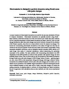
where eij = jrij i and A(r) is an arbitrary hydrodynamic field, and Ai = A(ri ). Expression (1.9) allows one to estimate the value of the derivative at a given point in terms of the value of the function at neighbouring points. The function F (r) is defined through ∇W (r) = −rF (r) A common selection for W (r) is the Lucy function,

(1.10)

7

DPD and other fluid particle models 30 25 20 15 10 5 0 0

Figure 1.1. line).

0.2

0.4

0.6

r

0.8

1

The functions W (r) (solid line), F (r) (bold line), and rF (r) (dotted

105 W (r) = 16πh3

r 1+3 h

r 1− h

3

(1.11)

from which the function F (r) follows 315 F (r) = 4πh5

r 1− h

2

,

F (r) ≥ 0

(1.12)

In Fig. 1.1 we plot the functions W (r), F (r), and rF (r). With the use of Eqn. (1.9) we can discretize the second order derivatives of the hydrodynamic equations (1.1), which correspond to the irreversible part of the dynamics. The equations also contain first order derivatives (∇P and ∇·v), which correspond to the reversible part of the dynamics. These first order derivatives are approximated by resorting to the definition of the density, Eqn. (1.8), and to the conservation of energy. The final discrete equations of hydrodynamics are (for simplicity we assume zero bulk viscosity) [7] r˙ i = vi mv˙ i =

" X Pi j

Ti S˙ i = −2κ

#

Pj 5η X Fij (vij + eij eij ·vij ) + 2 Fij rij − 2 3 j di dj di dj

X Fij j

di dj

Tij +

5η X Fij 2 vij + (eij ·vij )2 6 j di dj

(1.13)

Here, Pi , Ti are the pressure and temperature of the fluid particle i, which are functions of di , Si through the equilibrium equations of state.

8 In addition, vij = vi − vj , and Tij = Ti − Tj . It is easily shown that the above model conserves mass, momentum and energy and that the total entropy is a non-decreasing function of time. The physical picture that emerges from these equations is very appealing and closely resembles the interpretation of dissipative particles in DPD. Particles of constant mass m move according to their velocities and exert forces of a range h to each other of different nature. First, a repulsive force directed along the line joining the particles that has a magnitude given by the pressure and densities of the particles. Roughly speaking, the larger is the pressure in a given region, the higher the repulsion between them. The fluid particles are also subject to friction forces that depend on the relative velocities of the particles. As opposed to the friction force of the DPD model, there is a component of this forces, directly proportional to v ij that breaks the conservation of total angular momentum. If one wishes to respect this conservation law, then it is necessary to introduce in the model a spin variable associated to every particle [19]. For a sufficiently large number of particles, the violation of angular momentum is negligible [19]. The terms in the entropy equation have the same meaning as those in the original equation (1.1), that is, heat conduction and viscous heating. The heat conduction term tries to reduce temperature differences between particles by suitable energy exchange [18], whereas the viscous heating term ensures that the kinetic energy dissipated by the friction forces is transformed into internal energy of the fluid particles. The above model can be regarded as one more version of SPH, of which there are many [15, 16, 17, 18]. However, to our knowledge this is the first model that strictly respects the Second Law. As it is apparent from the GENERIC framework, the Second Law (expressed as a matrix M (x) which is positive definite) and the Fluctuation-Dissipation theorem are closely related. It is not possible to have properly defined thermal fluctuations in a model if the Second Law is not respected exactly. The interesting feature of the SPH model presented above is that it allows for the inclusion of thermal fluctuations. This cannot be achieved in the rest of current implementations of SPH. Therefore, the above model is the first SPH implementation that can be used in the mesoscopic realm where thermal fluctuations are important. Needless to say that many physical processes of complex fluids at mesoscopic scales are diffusion dominated processes due to thermal fluctuations. The set of deterministic equations (1.13) can be cast in the GENERIC form (1.2) [7]. The corresponding stochastic form (1.3) will be given below. First, one postulates the following form for the thermal noises d˜ x = {0, d˜ vi , dS˜i }. Note that we do not assume any fluctuation in

9


the position because we want to respect the purely reversible equation r˙ i = vi . The velocity and entropy random terms are postulated to be md˜ vi =

X

Aij dWij ·eij

j

1 Ti dS˜i = − 2

X

Aij dWij : eij vij +

j

X

Cij dVij

(1.14)

j

We have introduced, for each pair i, j of particles, a matrix of independent increments of the Wiener process dW ij . In Eqn. (1.14) we have also introduced an independent increment of the Wiener process for each pair of particles, dVij . This term will give rise to the heat conduction terms. Finally, the functions Aij , Cij might depend on the state of the system through the positions and entropy of the particles. We postulate the following symmetry properties, that will ensure momentum and energy conservation dWij dVij Aij Cij

= = = =

dWji −dVji Aji Cji

(1.15)

The independent increments of the Wiener processes satisfy the following Itô mnemotechnical rules ββ αα dWii 0 dW 0 jj 0

0

dVii0 dVjj 0 αα0 dWii 0 dVii0

0 0

= [δij δi0 j 0 + δij 0 δi0 j ]δ αβ δ α β dt = [δij δi0 j 0 − δij 0 δi0 j ]dt = 0

(1.16)

which respect the symmetries (1.15) under particle interchange. As a convention, superindices refer to tensorial components while subindices label different particles. The procedure now is to construct the matrix M through the FluctuationDissipation theorem (1.5), compute the gradient of the entropy and then construct the irreversible part of the dynamics M ∂S ∂x . By comparing with the discretization in Eqn. (1.13), one finds the appropriate forms for the unknown noise amplitudes Aij , Cij , which are

Aij

=

"

Ti Tj 5η Fij 8kB Ti + T j 3 di dj

#1/2

10 Cij =

"

Fij 4κkB Ti Tj di dj

#1/2

(1.17)

The final stochastic equations (1.3) for the fluid particle model are given by [7] dri = vi dt mdvi =

" X Pi j

Ti dSi =

#

Pj 5η X Fij + F r dt − (vij + eij eij ·vij ) dt + md˜ vi ij ij 3 j di dj d2i d2j

X Fij 5η X Fij 2 vij + (eij ·vij )2 dt − 2κ Tij dt + Ti dS˜i(1.18) 6 j di dj d d i j j

where we have neglected, for the sake of the presentation, small terms of the order of kB /Ci , where Ci is the heat capacity at constant volume of particle i. These terms are important if one wishes to obtain exact energy conservation [7]. We understand the model in Eqns. (1.18) as the “proper” DPD model valid for the simulation of Newtonian fluids at mesoscopic scales when thermal fluctuations are important. There have been several precursor models that have tried to generalize DPD in order to incorporate energy transport [20, 21], and pressure forces [22], but none of them can be understood as fully thermodynamically consistent. A previous attempt to formulate a thermodynamically consistent model [23] showed the general structure of such a model but the connection with the macroscopic hydrodynamic equations was not evident. The model in Eqns. (1.18) has a similar simplicity as the original DPD model but with a sounded physical meaning. It should be regarded as an SPH model with thermal fluctuations included in a consistent way. The model solves all the conceptual problems mentioned in the introduction. In particular, the pressure and any other thermodynamic information is introduced as an input. The conservative forces of the original model become physically sounded pressure forces. Energy is conserved and we can study transport of energy in the system. The Second Law is satisfied. The transport coefficients are input of the model [24]. The range functions of DPD have now very specific forms (see Fig. 1.1). The particles have a physical size given by its physical volume and it is possible to specify the physical scale being simulated. It has been checked through simulations that, if the fluid particles are large, the amplitude of the thermal fluctuations is negligible, in accordance with the usual notions of equilibrium statistical mechanics.


2.2

11

Voronoi fluid particles

The second model of fluid particles that we have developed in Ref. [6] was inspired by the work of Flekkøy, Coveney and De Fabrittis [25], who derived a model of fluid particles based on the Voronoi tessellation. A comparison between the models of both groups has been done in Ref. [12] and the conclusion is that the implementation in Ref. [6] produces slightly better results than those of Ref. [25] as a result of a better approximation of spatial derivatives. The idea in the Voronoi fluid particle model is to discretize the continuum hydrodynamic equations in a set of moving nodes that move with the flow. The nodes define the centers of an evolving Voronoi tessellation. The Voronoi tessellation associates to every node that region of space that is closer to it than to any other node. In this way, a cellular division of space is accomplished, see Fig. 1.2.

Figure 1.2. Voronoi tessellation in a periodic box. Every cell represents a thermodynamic portion of fluid.

The discretization we have followed in Ref. [6] is basically a finite volume discretization, that is, the continuum equations are integrated over each Voronoi cell, and through the divergence theorem, surface terms provide the rate of change of the extensive variables in the cell. In order to cast the model within the GENERIC framework, a small term in the momentum equation had to be added. The interested reader can look at the original work for the detailed equations [6].

12 It must be remarked that the physical idea and motivation of this Voronoi model, as well as its status as a fluid particle model, is essentially the same as the smooth fluid particle model. Of course, the question then arises about which model is the best one. At present, this question requires more investigation. On one hand, the implementation of the Voronoi tessellation is far from trivial, although there are efficient and freely available subroutines on the web. On the other hand, the number of interacting neighbours for the Voronoi fluid particles is much smaller than those for the soft fluid particles. For example, the typical number of neighbours required in the soft fluid particle model in order to recover the continuum results is 60 or larger in two dimensions, as compared to the typical number of six neighbours in the Voronoi model. The computational burden of constructing the tessellation at each time step may be compensated by the much smaller number of neighbours. There is also a problem with the soft fluid particles which is the unphysical forces that appear in the model when all the pressures of the particles are equal. In thermomechanical equilibrium we should have no motion irrespective of the location of the particles. If we set P i = P , equal temperatures and zero velocities in Eqn. (1.13), we still have remnant forces on the particles unless the particles distribute themselves in regular crystalline positions. One consequence of this artifact is the tendency to form regular crystals at equilibrium. This is a numerical artifact that produces small elastic components in the system. This effect is reduced by increasing the number of neighbours of each fluid particle. The ultimate origin of this remnant forces is the fact that the sum of the volumes of each fluid particle is not the container’s volume, but rather a slightly fluctuating quantity. This is at variance with the Voronoi fluid particles, where the sum of the volumes of each cell equals the container volume. No regular crystals are observed in the Voronoi model at equilibrium. Finally, the implementation of boundary conditions in the soft particle model requires some consideration. As in any SPH simulation, one has to test and fine tune the boundary conditions in order to recover the desired properties (no velocity slip or no temperature jumps at solid walls, etc.) [26]. These problems are not expected to appear in the Voronoi model, because there the implementation of boundary conditions is straightforward (one simply specifies fluxes at the walls of the cells, for example). In our opinion, the Voronoi model is conceptually more elegant and superior to the soft particle model, and perhaps even faster due to the smaller number of neighbours. However, the complexity of programming


13

a 3D Voronoi code as opposed to the simplicity of the smooth fluid particle code still leaves room for applications of the soft particle model.

3.

Complex fluids

We have seen how the original and simple DPD model can be put in a more firm ground by understanding the dissipative particles as truly fluid particles described with thermodynamic variables. As a result, a Newtonian fluid can be easily simulated. Of course, DPD was invented not to solve the Navier-Stokes equations but rather to simulate complex fluids with possibly non-Newtonian behaviour. As we have mentioned in the introduction, the strategy followed by DPD users has been to modify the conservative forces between dissipative particles in order to “complexify” the fluid. In an interesting paper, Warren has reviewed and commented on the applications of DPD to complex fluids [27]. In the following we outline two different approaches for the simulation of complex fluids based on the concept of fluid particles. The first one is based on the construction of objects or mesostructures out of fluid particles. The second approach relies on the concept of internal variables.

3.1

Mesostructures through conservative interactions

The first approach is the one followed up to now by the DPD community, which is to construct mesostructures by postulating additional conservative interactions between the dissipative particles. In this way, different complex fluids can be modeled.

Colloidal suspensions. Colloidal particles are constructed by freezing fluid particles inside certain region, typically spheres or ellipsoids, and moving those particles as a rigid body. The idea was pioneered by Koelman and Hoogerbrugge [28] and has been explored in more detail by Boek et al. [29]. The simulation results for shear thinning curves of spherical particles compare very well with experimental results for volume fractions below 30% [29]. At higher volume fractions somewhat inconsistent results are obtained, which can be attributed to several factors. For example, it is by no means clear that a stick boundary condition arises from the interaction friction between the solvent and the colloid. Also, being constructed out of fluid particles, the colloidal particles are to certain degree “soft balls” that can interpenetrate. In this sense, the radius of the colloidal particles is not well-defined. Perhaps a steep potential of (hard sphere-like) between colloidal particles is a better model, although limited to spherically shaped particles

14 [30, 31, 32]. Because the colloidal particles move slowly as compared to the solvent particles, the steepness of the potential should not be a big problem. Another problem that appears at high volume fractions is that solvent particles are expelled from the region in between two colloidal particles. This has two consequences. First, the interaction is no longer hydrodynamically mediated, but occurs through the unphysical friction between the frozen fluid particles that constitute the two colloidal particles. In that case of short distances, it seems appropriate to model the interaction between colloidal particles through lubrication forces directly [33]. A second effect is the appearance of depletion forces, and this has been explored in Refs. [29, 32]. These depletion forces are unphysical and due solely to the discrete representation of the continuum solvent. It seems that a judicious selection of lubrication forces that would take into account the effects of the solvent when no dissipative particle exist in between two colloidal particles can eventually solve this problem. Finally, we note that the fluid particle method can resolve in principle the time scales of fluid momentum transport on the length scale of the colloidal particles or their typical interdistances. This time scale corresponds to the time scale of the decay of velocity autocorrelation function for submicronic colloidal particles. In this way, we expect that fluid particle models can be of good service in exploring small time scales in colloidal suspensions as those probed by Diffusive Wave Spectroscopy [34].

Polymer systems. Polymer molecules are constructed in DPD through the linkage of several dissipative particles through springs (either Hookean or FENE, [35]). Dilute polymer solutions are modeled by a set of polymer molecules interacting with a sea of fluid particles. The solvent quality can be varied by fine tuning the solvent-solvent and solvent-monomer interactions. In this way, a collapse transition has been observed in passing from a good solvent to a poor solvent [36]. Static scaling results for the radius of gyration and relaxation time with the number of beads are consistent with the Rouse/Zimm models [37]. The model displays hydrodynamic interactions and excluded volume interactions, depending on solvent quality. Rheological properties have been also studied showing a good agreement with known kinetic theory results [38, 39]. Polymer solutions confined between walls have also been modeled showing anisotropic relaxation in nanoscale gaps [40]. Polymer melts have been simulated showing that the static scaling and rheology correspond to the Rouse theory, as a result of screening of hydrodynamic and excluded volume interactions in the melt [37]. The model is unable to simulate entanglements due to the soft interactions between beads


15

that allow polymer crossing [37], although this effect can be partially controlled by suitable adjusting the length and intensity of the springs [41]. At this point, DPD appears as a well benchmarked model for the simulation of polymer systems. However, several conceptual problems still remain. For example, one would understand physically each dissipative particle in the polymer chain as a group of monomers. Actually, a coarse-graining of a 1D chain of bead and springs into “blobs” through a rigorous projection operator technique has shown that the interaction of such blobs is of the DPD type with an internal friction depending on relative velocities between blobs [42]. In recent years several interesting explicit coarse-graining of atomistic polymer molecules have appeared [43]. Most of them focus on deriving coarse-grained potentials between beads [44, 45, 46], but few of them have focused on the dissipative and stochastic aspects intrinsic of any coarse-graining [47]. Whereas coarsegrained potentials should produce the correct thermodynamic properties and structural properties above the bead scale, the dissipative forces will affect strongly the rheology of the system. We are not aware of any attempt to map the dissipative forces between explicitly coarse-grained realistic polymer molecules to a model of polymer molecules like those used in DPD. In other words, a microscopic basis for the DPD strings of monomers is still lacking. As a final point, we would like to mention the need to look for more general blob models that somehow include internal energy variables. Otherwise it is difficult to foresee how non-isothermal polymer melts can be simulated.

Phase separation. Immiscible fluid mixtures are modeled in DPD by assuming two types of particles [48]. Unequal particles repel each other more strongly than equal particles thus favouring phase separation. Starting from random initial conditions representing a high temperature miscible phase suddenly quenched, the domain growth has been investigated. In 2D and symmetric mixtures (equal fraction of each fluid), a crossover from a domain growth scaling as t 1/2 to t2/3 is observed [49]. This signals a crossover from a diffuse to inertial hydrodynamics regimes. For asymmetric quenches the growth law gives a scaling like t 1/2 [50]. It should be noted that in Ref. [51] a 3D symmetric mixture showed a lack of scaling corresponding to a viscous dominated growth. This was latter on elucidated through lattice Boltzmann simulations to be due most probably to finite size effects [53, 52]. Although lattice Boltzmann simulations allow to explore larger time scales than DPD [52], the simplicity of DPD modeling allows one to generalize easily to more complex systems in a way that lattice Boltzmann cannot. For example, mixtures of

16 homopolymers melts have been modeled with DPD [5]. Surface tension measurements allow for a mapping of the model to the Flory-Huggins theory [5]. In this way, thermodynamic information has been used to fix the model parameters of DPD. A recent more detailed analysis of this procedure has been presented in Refs. [54, 55] where a calculation of the phase diagram of monomer and polymer mixtures of DPD particles allowed to discuss the connection of the repulsion parameter difference and the Flory-Huggings parameter χ. Another successful application of DPD has been the simulation of microphase separation of diblock copolymers [56], that has allowed to discuss the pathway to equilibrium. This pathway is strongly affected by hydrodynamics [57]. In a similar way, simulations of rigid DPD dimers in a solution of solvent monomers has allowed to study the growth of amphiphilic mesophases and its behaviour under shear [58] and the self assembly of model membranes [59]. A general observation about the phase separation of liquid mixtures modeled with DPD so far is the isothermal character of such simulations. It would be very interesting to study non-isothermal situations by using thermodynamically consistent models for binary mixtures.

Other complex fluid systems. DPD has been applied to more complex situations like the dynamics of a drop at a liquid-solid interface [60], flow and rheology in the presence of polymers grafted to walls [61], and colloidal adsorption onto polymer coated surfaces [41]. Packing of cubically and spherically shaped granular materials has also been studied with DPD [62].

3.2

“Internal” variables

The second approach for the simulation of complex fluids with fluid particles is the natural continuation of the strategy we have pursued in the Newtonian fluid case. The idea is to start from well defined continuum equations for complex fluids. The crucial point is thermodynamic consistency, so a GENERIC version of the continuum equations is most welcome. Then a suitable discretization using either the Voronoi cells or the soft particles can be constructed in such a way that the GENERIC structure and, therefore, the thermodynamic consistency of the model is preserved even at the discrete level. In general, the continuum models of the GENERIC type for complex fluids typically involve additional structural or internal variables that are coupled with the conventional hydrodynamic variables. The coupling renders the behaviour of the fluid non-Newtonian and complex. For example, polymer melts are characterized by additional conformation

17


tensors, colloidal suspensions can be described by further concentration fields, mixtures are characterized by several density fields (one for each chemical specie), emulsions are described with the amount and orientation of interface, etc. All these continuum models rely on the hypothesis of local equilibrium and, therefore, the fluid particles are regarded as thermodynamic subsystems. The physical picture that emerges from these fluid particles is that they represent “large” portions of the fluid and therefore, the scale of these fluid particles is supramolecular. This allows one to study larger time scales than the less coarse models of the previous section. The price, of course, is the need for a deep understanding of the physics at this more coarse-grained level, which appears in the form of entropy and energy functionals depending on internal variables and kinematic and dissipative matrices L(x), M (x) describing the complex coupling of the internal microstructure and flow. In order to model polymer solutions, for example, we have developed a model of fluid particles inspired by a previous model introduced by Ten Bosch [63]. In this DPD model the dissipative particles include an elongation vector, representing the average elongation of polymer molecules. Although the Ten Bosch model has all the problems of the original DPD model, it can be cast into a thermodynamically consistent model for dilute polymer solutions rather simply [64]. Thanks to its thermodynamic consistency, the model allows to study non-isothermal situations. A graphical view of the fluid particle for polymer solutions is given in Fig. 1.3

Q

Figure 1.3. A fluid particle containing N d dumbbell molecules with a typical orientation Q. These two further variables, N d and Q characterize along with ri , vi , Vi , Si the state of the fluid particle, and their dynamics is specified from simple physical grounds: fluid particles exchange dumbbells due to chemical potential differences and the vector Q changes due to the underlying Brownian motion of the dumbbells and the extensional state of the fluid particle.

18 Another example where the strategy of internal variables is successful is in the simulation of chemically reacting mixtures. Chemically reacting mixtures are not easily implemented with the usual approach taken by DPD in order to model mixtures. In DPD, mixtures are represented by “red” and “blue” particles. It is not trivial to specify a chemical reaction in which, for example, two red particles react with a blue particle to form a “green” particle. In this case, it is better to start from the well established continuum equations for chemical reactions [8, 65]. The resulting discrete model consists on fluid particles that have as additional variable the fraction of component red and blue inside the fluid particle. There are diffusion terms that change this fraction depending on the difference between chemical potentials of neighbouring particles, and there are simple reaction terms, that can be expressed in measurable reaction rates [66]. These two examples show how one can address viscoelastic flow problems and chemical reacting fluids with a simple methodology that involves fluid particles with internal variables. The idea can, of course, be applied to other complex fluids where the continuum equations are known.

Acknowledgments I would like to thank Marisol Ripoll and Mar Serrano for the very good times we had discussing about DPD. A first version of this material appeared in electronic format in the Fourth SIMU Newsletter (http://simu.ulb.ac.be/newsletters/newsletter.html). This work has been partially supported by the project BFM2001-0290 of the Spanish Ministerio de Ciencia y Tecnolog´ıa.

References [1] P. J. Hoogerbrugge and J. M. V. A. Koelman. Simulating microscopic hydrodynamic phenomena with dissipative particle dynamics. Europhys. Lett., 19 155 (1992). [2] P. Espa˜ nol and P. Warren. Statistical mechanics of dissipative particle dynamics. Europhys. Lett., 30, 191 (1995). [3] P. Espa˜ nol. Hydrodynamics for dissipative particle dynamics. Phys. Rev. E, 52, 1734 (1995). [4] C. Marsh, G. Backx, and M.H. Ernst. Fokker-planck-boltzmann equation for dissipative particle dynamic. Europhys. Lett., 38, 411 (1997). C. Marsh, G. Backx, and M.H. Ernst. Static and dynamic properties of dissipative particle dynamics. Phys. Rev. E, 56, 1976

REFERENCES

[5]

[6] [7] [8] [9] [10]

[11]

[12]

[13] [14] [15]

[16]

19

(1997). M. Ripoll, P. Espa˜ nol, and M. H. Ernst. Dissipative particle dynamics with energy conservation: Heat conduction. Int. J. of Mod. Phys. C, 9, 1329 (1998). G. T. Evans. Dissipative particle dynamics: Transport coefficients. J. Chem. Phys, 110, 1338 (1999). A. J. Masters and P. B. Warren. Kinetic theory for dissipative particle dynamics: The importance of collisions. Europhys. Lett., 48, 1 (1999). M. Ripoll, M. H. Ernst, and P. Espa˜ nol. Large scale and mesoscopic hydrodynamic for dissipative particle dynamics. J. Chem. Phys, 115, 7271 (2001). R. D. Groot and P. B. Warren. Dissipative particle dynamics: Bridging the gap between atomistic and mesoscopic simulation. J. Chem. Phys, 107, 4423 (1997). M. Serrano and P. Espa˜ nol. Thermodynamically consistent mesoscopic fluid particle model. Phys. Rev. E, 65:46115 (2001). P. Espa˜ nol and M. Revenga. Smoothed Dissipative Particle Dynamics, preprint. L. D. Landau and E. M. Lifshitz, Fluid Mechanics, (Pergamon Press, 1959). S. R. de Groot and P. Mazur, Non-equilibrium Thermodynamics (North Holland Publishing Company, Amsterdam, 1964). ¨ M. Grmela and H. C. Ottinger. Dynamics and thermodynamics of complex fluids. I. Development of a general formalism, Phys. ¨ Rev. E, 56, 6620 (1997). H. C. Ottinger and M. Grmela. Dynamics and thermodynamics of complex fluids. II. Ilustrations of a general formalism, Phys. Rev. E, 56, 6633 (1997). ¨ H. C. Ottinger. General Projection operator formalism for the dynamics and thermodynamics of complex fluids, Phys. Rev. E, 57, 1416 (1998). M. Serrano, G. de Fabritiis, P. Espa˜ nol, Eirik Flekkoy and P.V. Coveney. Mesoscopic dynamics of Voronoi fluid particles, to appear in J. Phys. A: Math. Gen. (2002). L.B. Lucy. A numerical testing of the fission hypothesis Astron. J. 82, 1013 (1977). J.J. Monaghan. Smoothed Particle Hydrodynamics. Annu. Rev. Astron. Astrophys. 30, 543 (1992). H. Takeda, S.M. Miyama, and M. Sekiya, Prog. Theor. Phys. 92, Numerical simulation of viscous flow by Smoothed Particle Hydrodynamics. 939 (1994). H.A. Posch, W.G. Hoover, and O. Kum. Steady state shear flows via nonequilibrium molecular dynamics and smooth-particle applied

20 mechanics. Phys. Rev. E 52, 1711 (1995). O. Kum, W.G. Hoover, and H.A. Posch. Viscous conducting fows with smooth-particle applied mechanics Phys. Rev. E 52, 4899 (1995). [17] S.J. Watkins, A.S. Bhattal, N. Francis, J.A. Turner, A.P. Whitworth. A new prescription for viscosity in Smoothed Particle Hydrodynamics. Astron. Astrophys. Suppl. Ser. 119, 177 (1996). [18] P.W. Cleary and J.J. Monaghan. Conduction modelling using Smoothed Particle Hydrodynamics. J. Comp. Phys. 148, 227 (1999). [19] P. Espa˜ nol. Fluid particle model. Phys. Rev. E, 57, 2930 (1998). P. Espa˜ nol. Fluid particle dynamics: a syntehsis of dissipative particle dynamics and smoothed particle dynamics. Europhys. Lett. 39, 606 (1997). [20] J. Bonet-Avalós and A. D. Mackie. Dissipative particle dynamics with energy conservation. Europhys. Lett., 40, 141 (1997). J. BonetAvalós and A. D. Mackie. Dynamic and transport properties of dissipative particle dynamics with energy conservation. J. Chem. Phys, 11, 5267 (1999). [21] P. Espa˜ nol. Dissipative particle dynamics with energy conservation. Europhys. Lett., 40, 631 (1997). M. Ripoll, P. Espa˜ nol, and M. H. Ernst. Dissipative particle dynamics with energy conservation: Heat conduction. Int. J. of Mod. Phys. C, 9, 1329 (1998). [22] I. Pagonabarraga and D. Frenkel. Dissipative particle dynamics for interacting systems. J. Chem. Phys, 115, 5015 (2001). ¨ [23] P. Espa˜ nol, M. Serrano, and H. C. Ottinger. Thermodinamically admisible form for discrete hydrodynamics. Phys. Rev. Lett., 83:4552, 1999. [24] The input values of the transport coefficients are realized only in the long wavelength limit, of course. [25] E. G. Flekkøy and P. V. Coveney. From molecular to dissipative particle dynamics. Phys. Rev. Lett., 83 1775 (1999). E. G. Flekkøy, P. V. Coveney, and G. D. Fabritiis. Foundations of dissipative particle dynamics. Phys. Rev. E, 62, 2140 (2000). [26] P.W. Randles and L.D. Libersky. Smoothed Particle Hydrodynamics: Some recent improvements and applications Comput. Methods Appl. Mech. Engrg. 139, 375 (1996). [27] P. Warren. Dissipative particle dynamics. Curr. Opinion Colloid Interface Sci.,3, 620 (1998).

REFERENCES

21

[28] J. M. V. A. Koelman and P. J. Hoogerbrugge. Dynamic simulations of hard-sphere suspensions under steady state shear. Europhys. Lett., 21, 363 (1993). [29] E. S. Boek, P. V. Coveney, and H.N.W. Lekkerkerker. Computer simulation of rheological phenomena in dense colloidal suspensions with dissipative particle dynamics. J. Phys.: Condens. Matter, 8, 9509 (1996). E. S. Boek, P. V. Coveney, H. N. W. Lekkerkerker, and P. van der Schoot. Simulating the rheology of dense colloidal suspensions using dissipative particle dynamics. Phys. Rev. E, 55, 3124 (1997). E. S. Boek and P. van der Schoot. Resolution effects in dissipative particle dynamics simulations. Int. J. of Mod. Phys. C, 9, 1307 (1998). [30] W. Dzwinel and D. A. Yuen. A two-level, discrete-particle approach for simulating ordered colloidal structures. Journal of Colloid and Interface Science, 225, 179 (2000). [31] W. Dzwinel and D. A. Yuen. A two-level, discrete-particle approach for large-scale simulation of colloidal aggregates. Int. J. of Mod. Phys. C, 11, 1037 (2000). [32] M. Whittle and E. Dickinson, On simulating colloids by dissipative particle dynamics: Issues and complications, J. Colloid and Interface Science 242, 106 (2001) [33] J.R. Melrose, J.H. van Vliet, and R.C. Ball. Continuous shear thickening and colloid surfaces. Phys. Rev. Lett. 77, 4660 (1996). [34] J.X. Zhu, D.J. Durian, J. M¨ uller, D.A. Weitz, and D.J. Pine, Phys. Rev. Lett. 68, 2559 (1992). M. Kao, A. Yodh, and D.J. Pine, Phys. Rev. Lett. 70, 242 (1993). [35] A. G. Schlijper, P. J. Hoogerbrugge, and C. W. Manke. Computer simulation of dilute polymer solutions with the dissipative particle dynamics method. J. Rheol., 39, 567 (1995). [36] Y. Kong, C. W. Manke, W. G. Madden, and A. G. Schlijper. Effect of solvent qualityon the conformation and relaxation of polymers via dissipative particle dynamics. J. Chem. Phys, 107, 592 (1997). [37] N. A. Spenley. Scaling laws for polymers in dissipative particle dynamics. Europhys. Lett., 49, 534 (2000). [38] Y. Kong, C. W. Manke, W. G. Madden, and A. G. Schlijper. Modeling the rheology of polymer solutions by dissipative particle dynamics. Tribology Letters, 3, 133 (1997). [39] A. G. Schlijper, C. W. Manke, W. D. Madden, and Y. Kong. Computer simulation of non-newtonian fluid rheology. Int. J. of Mod. Phys. C, 8, 919 (1997).

22 [40] Y. Kong, C. W. Manke, W. G. Madden, and A. G. Schlijper. Simulation of a confined polymer on solution using the dissipative particle dynamics method. Int. J. Thermophys., 15, 1093 (1994). [41] J. B. Gibson, K. Chen, and S. Chynoweth. Simulation of particle adsoption onto a polymer-coated using the disspative particle dynamics method. Journal of Colloid and Interface Science, 206, 464 (1998). J. B. Gibson, K. Zhang, K. Chen, S. Chynoweth, and C. W. Manke. Simulation of colloid-polymer systems using disspative particle dynamics, (Preprint).1999. [42] P. Espa˜ nol. Dissipative particle dynamics for a harmonic chain: A first-principles derivation. Phys. Rev. E, 53, 1572 (1996). [43] A. Uhlherr and D.N. Theodorou, Hierarchical simulation approach to structure and dynamics of polymers. Current Opinion in Solid State & Materials Science, 3, 544 (1998). [44] W. Tschöp, K. Kremer, J. Batoulis, T. Burger, and O. Hahn, Simulation of polymer melts. I. Coarse-graining procedure for polycarbonates. Acta Polymer, 49, 61 (1998). [45] H. Meyer, O. Biermann, R. Faller, D. Reith, and F. M¨ uller-Plathe. Coarse graining of nonbonded inter-particle potentials using automatic simplex optimization to fit structural properties. J. Chem. Phys. 113, 6264 (2000). [46] R.L.C. Akkermans and W.J. Briels. Coarse-grained interactions in polymer melts: A variational approach. J. Chem. Phys. 115, 6210 (2001). [47] R.L.C. Akkermans and W.J. Briels. Coarse-grained dynamics of one chain in a polymer melt. J. Chem. Phys. 113, 6409 (2000). [48] P. V. Coveney and K. Novik. Computer simulations of domain growth and phase separation in two-dimensional binary immiscible fluids using dissipative particle dynamics. Phys. Rev. E, 54, 5134 (1996). P. V. Coveney and K. Novik. Erratum: Computer simulations of domain growth and phase separation in two-dimensional binary immiscible fluids using dissipative particle dynamics. Phys. Rev. E, 55, 4831 (1997). K.E. Novik and P.V. Coveney. Finitedifference methods for simulation models incorporating nonconservative forces. J. Chem. Phys. 109, 7667 (1998). [49] K. E. Novik and P. V. Coveney. Using dissipative particle dynamics to model binary immiscible fluids. Int. J. Mod. Phys. C 8, 909 (1997). [50] K. E. Novik and P. V. Coveney. Spinodal decomposition off ofcritical quenches with a viscous phase using dissipative particle dy-

REFERENCES

[51]

[52] [53]

[54]

[55]

[56] [57]

[58]

[59] [60]

[61] [62]

[63]

[64]

23

namics in two and three spatial dimensions. Phys. Rev. E, 61, 435 (2000). S. I. Jury, P. Bladon, S. Krishna, and M. E. Cates. Test of dynamical scaling in three-dimensional spinodal decomposition. Phys. Rev. E,59 R2535, 1999. V.M. Kendon, J-C. Desplat, P. Bladon, and M.E. Cates Phys. Rev. Lett. 83, 576 (1999). M. E. Cates, V. M. Kendon, P. Bladon, J-C. Desplat. Inertia, coarsening and fluid motion in binary mixtures Faraday Disc. Roy. Chem. Soc. 112, 1 (1999). S. M. Willemsen, T. J. H. Vlugt, H. C. J. Hoefsloot, and B. Smit. Combining dissipative particle dynamics and monte carlo techniques. J. Comp. Phys., 147, 507 (1998). C. M. Wijmans, B. Smit, and R. D. Groot. Phase behavior of monomeric mixtures and polymer solutions with soft interaction potentials. J. Chem. Phys, 114, 7644 (2001). R. D. Groot, T. J. Madden. Dynamic simulation of diblock copolymer microphase separation. J. Chem. Phys, 108, 8713 (1997). R. D. Groot, T. J. Madden, and D. J. Tildesley. On the role of hydrodynamic interactions in block copolymer microphase separation. J. Chem. Phys, 110, 9739 (1999). S. Jury, P. Bladon, M. Cates, S. Krishna, M. Hagen, N. Ruddock, and P. Warren. Simulation of amphiphilic mesophases using dissipative particle dynamics. Phys. Chem. Chem. Phys. 1, 2051 (1999). M. Venturoli and B. Smit. Simulating the self-assembly of model membranes. Phys. Chem. Comm. 10 (1999). J.L. Jones, M. Lal, N. Ruddock, and N. A. Spenley. Dynamics of a drop at a liquid/solid interface in simple shear fields: A mesoscopic simulation study. Faraday Discussions, 112, 129 (1999). P. Malfreyt, D.J. Tildesley, Dissipative particle dynamics of grafted polymer chains between two walls. Langmuir, 16, 4732 (2000). J.A. Elliott and A.H. Windle. A dissipative particle dynamics method for modeling the geometrical packing of filler particles in polymer composites. J. Chem. Phys. 113, 10367 (2000). B.I.M. ten Bosch, On an extension of Dissipative Particle Dynamics for viscoelastic flow modelling, J. Non-Newtonian Fluid Mech. 83, 231 (1999). P. Espa˜ nol and E.G. Flekkøy, Smoothed dissipative particle dynamics for viscoelastic flows, preprint (2002).

24 [65] L. E. Reichl, A modern course in statistical physics (Univ. of Texas Press, Austin 1980) [66] P. Espa˜ nol, Fluid particle model for chemical reactions, preprint (2002).