Foundations of Dissipative Particle Dynamics

Foundations of Dissipative Particle Dynamics Eirik G. Flekkøy1 , Peter V. Coveney2 and Gianni De Fabritiis2

arXiv:cond-mat/0002174v1 [cond-mat.soft] 11 Feb 2000

1

Department of Physics, University of Oslo P.O. Box 1048 Blindern, 0316 Oslo 3, Norway 2 Centre for Computational Science, Queen Mary and Westfield College, University of London, London E1 4NS, United Kingdom (February 1, 2008) We derive a mesoscopic modeling and simulation technique that is very close to the technique known as dissipative particle dynamics. The model is derived from molecular dynamics by means of a systematic coarse-graining procedure. This procedure links the forces between the dissipative particles to a hydrodynamic description of the underlying molecular dynamics (MD) particles. In particular, the dissipative particle forces are given directly in terms of the viscosity emergent from MD, while the interparticle energy transfer is similarly given by the heat conductivity derived from MD. In linking the microscopic and mesoscopic descriptions we thus rely on the macroscopic description emergent from MD. Thus the rules governing our new form of dissipative particle dynamics reflect the underlying molecular dynamics; in particular all the underlying conservation laws carry over from the microscopic to the mesoscopic descriptions. We obtain the forces experienced by the dissipative particles together with an approximate form of the associated equilibrium distribution. Whereas previously the dissipative particles were spheres of fixed size and mass, now they are defined as cells on a Voronoi lattice with variable masses and sizes. This Voronoi lattice arises naturally from the coarse-graining procedure which may be applied iteratively and thus represents a form of renormalisation-group mapping. It enables us to select any desired local scale for the mesoscopic description of a given problem. Indeed, the method may be used to deal with situations in which several different length scales are simultaneously present. We compare and contrast this new particulate model with existing continuum fluid dynamics techniques, which rely on a purely macroscopic and phenomenological approach. Simulations carried out with the present scheme show good agreement with theoretical predictions for the equilibrium behavior. Pacs numbers: 47.11.+j 47.10.+g 05.40.+j

tions are usually unavailable and instead it is necessary to base the modeling approach on a microscopic (that is on a particulate) description of the system, thus working from the bottom upwards, along the general lines of the program for statistical mechanics pioneered by Boltzmann [2]. Molecular dynamics (MD) presents itself as the most accurate and fundamental method [3] but it is far too computationally intensive to provide a practical option for most hydrodynamic problems involving complex fluids. Over the last decade several alternative ‘bottom up’ strategies have therefore been introduced. Hydrodynamic lattice gases [4], which model the fluid as a discrete set of particles, represent a computationally efficient spatial and temporal discretization of the more conventional molecular dynamics. The lattice-Boltzmann method [5], originally derived from the lattice-gas paradigm by invoking Boltzmann’s Stosszahlansatz, represents an intermediate (fluctuationless) approach between the top-down (continuum) and bottom-up (particulate) strategies, insofar as the basic entity in such models is a single particle distribution function; but for interacting systems even these lattice-Boltzmann methods can be subdivided into bottom-up [6] and top-down models [7]. A recent contribution to the family of bottom-up approaches is the dissipative particle dynamics (DPD) method introduced by Hoogerbrugge and Koelman in

I. INTRODUCTION

The non-equilibrium behavior of fluids continues to present a major challenge for both theory and numerical simulation. In recent times, there has been growing interest in the study of so-called ‘mesoscale’ modeling and simulation methods, particularly for the description of the complex dynamical behavior of many kinds of soft condensed matter, whose properties have thwarted more conventional approaches. As an example, consider the case of complex fluids with many coexisting length and time scales, for which hydrodynamic descriptions are unknown and may not even exist. These kinds of fluids include multi-phase flows, particulate and colloidal suspensions, polymers, and amphiphilic fluids, including emulsions and microemulsions. Fluctuations and Brownian motion are often key features controlling their behavior. From the standpoint of traditional fluid dynamics, a general problem in describing such fluids is the lack of adequate continuum models. Such descriptions, which are usually based on simple conservation laws, approach the physical description from the macroscopic side, that is in a ‘top down’ manner, and have certainly proved successful for simple Newtonian fluids [1]. For complex fluids, however, equivalent phenomenological representa1

1992 [8]. Although in the original formulation of DPD time was discrete and space continuous, a more recent reinterpretation asserts that this model is in fact a finitedifference approximation to the ‘true’ DPD, which is defined by a set of continuous time Langevin equations with momentum conservation between the dissipative particles [9]. Successful applications of the technique have been made to colloidal suspensions [10], polymer solutions [11] and binary immiscible fluids [12]. For specific applications where comparison is possible, this algorithm is orders of magnitude faster than MD [13]. The basic elements of the DPD scheme are particles that represent rather ill-defined ‘mesoscopic’ quantities of the underlying molecular fluid. These dissipative particles are stipulated to evolve in the same way that MD particles do, but with different inter-particle forces: since the DPD particles are pictured to have internal degrees of freedom, the forces between them have both a fluctuating and a dissipative component in addition to the conservative forces that are present at the MD level. Newton’s third law is still satisfied, however, and consequently momentum conservation together with mass conservation produce hydrodynamic behavior at the macroscopic level. Dissipative particle dynamics has been shown to produce the correct macroscopic (continuum) theory; that is, for a one-component DPD fluid, the Navier-Stokes equations emerge in the large scale limit, and the fluid viscosity can be computed [14,15]. However, even though dissipative particles have generally been viewed as clusters of molecules, no attempt has been made to link DPD to the underlying microscopic dynamics, and DPD thus remains a foundationless algorithm, as is that of the hydrodynamic lattice gas and a fortiori the lattice-Boltzmann method. It is the principal purpose of the present paper to provide an atomistic foundation for dissipative particle dynamics. Among the numerous benefits gained by achieving this, we are then able to provide a precise definition of the term ‘mesoscale’, to relate the hitherto purely phenomenological parameters in the algorithm to underlying molecular interactions, and thereby to formulate DPD simulations for specific physicochemical systems, defined in terms of their molecular constituents. The DPD that we derive is a representation of the underlying MD. Consequently, to the extent that the approximations made are valid, the DPD and MD will have the same hydrodynamic descriptions, and no separate kinetic theory for, say, the DPD viscosity will be needed once it is known for the MD system. Since the MD degrees of freedom will be integrated out in our approach the MD viscosity will appear in the DPD model as a parameter that may be tuned freely. In our approach, the ‘dissipative particles’ (DP) are defined in terms of appropriate weight functions that sample portions of the underlying conservative MD particles, and the forces between the dissipative particles are obtained from the hydrodynamic description of the MD

system: the microscopic conservation laws carry over directly to the DPD, and the hydrodynamic behavior of MD is thus reproduced by the DPD, albeit at a coarser scale. The mesoscopic (coarse-grained) scale of the DPD can be precisely specified in terms of the MD interactions. The size of the dissipative particles, as specified by the number of MD particles within them, furnishes the meaning of the term ‘mesoscopic’ in the present context. Since this size is a freely tunable parameter of the model, the resulting DPD introduces a general procedure for simulating microscopic systems at any convenient scale of coarse graining, provided that the forces between the dissipative particles are known. When a hydrodynamic description of the underlying particles can be found, these forces follow directly; in cases where this is not possible, the forces between dissipative particles must be supplemented with the additional components of the physical description that enter on the mesoscopic level. The DPD model which we derive from molecular dynamics is formally similar to conventional, albeit foundationless, DPD [14]. The interactions are pairwise and conserve mass and momentum, as well as energy [16,17]. Just as the forces conventionally used to define DPD have conservative, dissipative and fluctuating components, so too do the forces in the present case. In the present model, the role of the conservative force is played by the pressure forces. However, while conventional dissipative particles possess spherical symmetry and experience interactions mediated by purely central forces, our dissipative particles are defined as space-filling cells on a Voronoi lattice whose forces have both central and tangential components. These features are shared with a model studied by Espa˜ nol [18]. This model links DPD to smoothed particle hydrodynamics [19] and defines the DPD forces by hydrodynamic considerations in a way analogous to earlier DPD models. Espa˜ nol et al. [20] have also carried out MD simulations with a superposed Voronoi mesh in order to measure the coarse grained inter-DP forces. While conventional DPD defines dissipative particle masses to be constant, this feature is not preserved in our new model. In our first publication on this theory [21], we stated that, while the dissipative particle masses fluctuate due to the motion of MD particles across their boundaries, the average masses should be constant. In fact, the DP-masses vary due to distortions of the Voronoi cells, and this feature is now properly incorporated in the model. We follow two distinct routes to obtain the fluctuationdissipation relations that give the magnitude of the thermal forces. The first route follows the conventional path which makes use of a Fokker-Planck equation [9]. We show that the DPD system is described in an approximate sense by the isothermal-isobaric ensemble. The second route is based on the theory of fluctuating hy2

drodynamics and it is argued that this approach corresponds to the statistical mechanics of the grand canonical ensemble. Both routes lead to the same result for the fluctuating forces and simulations confirm that, with the use of these forces, the measured DP temperature is equal to the MD temperature which is provided as input. This is an important finding in the present context as the most significant approximations we have made underlie the derivation of the thermal forces.

≡

r˙ k = Uk ≡ Pk /Mk

A. Definitions

Full representation of all the MD particles can be achieved in a general way by introducing a sampling function (1)

where the positions rk and rl define the DP centers, x is an arbitrary position and s(x) is some localized function. It will prove convenient to choose it as a Gaussian (2)

where the distance a sets the scale of the sampling function, although this choice is not necessary. The mass, momentum and internal energy E of the kth DP are then defined as X fk (xi )m, Mk = X

(4)

B. Equations of motion for the dissipative particles based on a microscopic description

i

Pk =

(3)

completes the definition of our dissipative particle dynamics. It is generally true that mass and momentum conservation suffice to produce hydrodynamic behavior. However, the equations expressing these conservation laws contain the fluid pressure. In order to get the fluid pressure a thermodynamic description of the system is needed. This produces an equation of state, which closes the system of hydrodynamic equations. Any thermodynamic potential may be used to obtain the equation of state. In the present case we shall take this potential to be the internal energy Ek of the dissipative particles, and we shall obtain the equations of motion for the DP mass, momentum and energy. Note that the internal energy would also have to be computed if a free energy had been chosen for the thermodynamic description. For this reason it is not possible to complete the hydrodynamic description without taking the energy flow into account. As a byproduct of this the present DPD also contains a description of the heat flow and corresponds to the recently introduced DPD with energy conservation [16,17]. Espa˜ nol previously introduced an angular momentum variable describing the dynamics of extended particles [18]: this is needed when forces are non-central in order to avoid dissipation of energy in a rigid rotation of the fluid. Angular momentum could be included on the same footing as momentum in the following developments. However for reasons both of space and conceptual economy we shall omit it in the present context, even though it is probably important in applications where hydrodynamic precision is important. In the following sections, we shall use the notation r, M , P and E with the indices k , l , m and n to denote DP’s while we shall use x, m, v and ǫ with the indices i and j to denote MD particles.

The essential idea motivating our definition of mesoscopic dissipative particles is to specify them as clusters of MD particles in such a way that the MD particles themselves remain unaffected while all being represented by the dissipative particles. The independence of the molecular dynamics from the superimposed coarsegrained dissipative particle dynamics implies that the MD particles are able to move between the dissipative particles. The stipulation that all MD particles must be fully represented by the DP’s implies that while the mass, momentum and energy of a single MD particle may be shared between DP’s, the sum of the shared components must always equal the mass and momentum of the MD particle.

s(x) = exp (−x2 /a2 )

fk (xi )ǫi ,

i

where xi and vi are the position and velocity of the ith MD particle, which are all assumed to have identical masses m, Pk is the momentum of the kth DP and VMD (rij ) is the potential energy of the MD particle pair ij, separated a distance rij . The particle energy ǫi thus contains both the kinetic and a potential term. The kinematic condition

II. COARSE-GRAINING MOLECULAR DYNAMICS: FROM MICRO TO MESOSCALE

s(x − rk ) . fk (x) = P l s(x − rl )

X

fk (xi )mvi ,

The fact that all the MD particles are represented at all instants in the coarse-grained P scheme is guaranteed by the normalization condition k fk (x) = 1. This implies directly that

i





X 1 1 1X fk (xi )  mvi2 + Mk Uk2 + Ek = VMD (rij ) 2 2 2 i j6=i

3

X

Mk = Pk =

k

X

mvi

rk

i

k

X

m

i

k

X

X

Ektot =

X1 k

2

Mk U2k + Ek



=

X

ǫi ;

l kl

fk (r )

(5)

rl

i

1

thus with mass, momentum and energy conserved at the MD level, these quantities are also conserved at the DP level. In order to derive the equations of motion for dissipative particle dynamics we now take the time derivatives of Eqs. (3). This gives X dMk f˙k (xi )m = dt i  X dPk f˙k (xi )mvi + fk (xi )Fi = dt i  X dEktot f˙k (xi )ǫi + fk (xi )ǫ˙i = dt i

(6)

rk

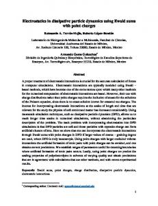
rl a2 /|r - r | k l

(7)

FIG. 1. The overlap region between two Voronoi cells is shown in grey. The sampling function fk (r) is shown in the top graph and the overlap function fkl (r) = (2/a2 )fk (r)fl (r) in the bottom graph. The width of the overlap region is a2 /|rk − rl | and its length is denoted by l.

(8)

These two functions are shown in Fig.1. Note that the scale of the overlap region is not a but a2 /|rk − rl |. Dissipative particle interactions only take place where the overlap function is non-zero. This happens along the dividing line which is equally far from the two particles. The contours of non-zero fkl thus define a Voronoi lattice with lattice segments of length lkl . This Voronoi construction is shown in Fig. 2 in which MD particles in the overlap region defined by fkl > 0.1, are shown, though presently not actually simulated as dynamic entities. The volume of the Voronoi cells will in general vary under the dynamics. However, even with arbitrary dissipative particle motion the cell volumes will approach zero only exceptionally, and even then the identities of the DP particles will be preserved so that they subsequently re-emerge.

The Gaussian form of s implies that s(x) ˙ = −(2/a2 )x˙ · xs(x). This makes it possible to write (9)

where the overlap function fkl is defined as fkl (x) ≡ (2/a2 )fk (x)fl (x), rkl ≡ (rk − rl ) and Ukl ≡ (Uk − Ul ), and we have rearranged terms so as to get them in terms of the centered variables (Uk + Ul ) 2 (r + rl ) k x′i = xi − . 2

rl

fkl(r)

where d/dt is the substantial derivative and Fi = mv˙ i is the force on particle i.

f˙k (xi ) = fkl (xi )(vi′ · rkl + x′i · Ukl )

rk

vi′ = vi −

(10) 1. Mass equation

Before we proceed with the derivation of the equations of motion it is instructive to work out the actual forms of fk (x) and fkl (x) in the case of only two particles k and l. Using the Gaussian choice of s we immediately get

The mass equation (6) takes the form X dMk ≡ M˙ kl dt

(13)

l

fk (x) =

1 1 + [exp ((x − (rk + rl )/2) · (rkl )/(a2 ))]2

. (11)

where M˙ kl =

i

The overlap function similarly follows: 1 fkl (x) = 2 cosh−2 2a

X

fkl (xi )m(vi′ · rkl + x′i · Ukl ) .

(14)

The vi′ term will be shown to be negligible within our approximations. The x′i ·Ukl -term however describes the geometric effect that the Voronoi cells do not conserve their

    rk + rl rkl · x− . (12) 2 a2 4

X

volume: The relative motion of the DP centers causes the cell boundaries to change their orientation. We will return to give this ‘boundary twisting’ term a quantitative content when the equations of motion are averaged–an effect which was overlooked in our first publication of this theory [21] where it was stated that hM˙ kl i = 0.

ij

fk (xi )Fij = − =− ≈−

X

fk (xi )Fji

ij

X

fk (xj + ∆xij )Fji

ij

X ij

fk (xj )Fji −

X ij

(∆xij · ∇fk (xi )) Fji

1X (∆xij · ∇fk (xi )) Fji 2 ij    X X 1 = fkl (xi )Fij ∆xij · rkl   2 ij

=−

Uk rk

(17)

l

where ∆xij = xi − xj , we have Taylor expanded fk (x) around xj and used a result similar to Eq. (9) to evaluate ∇fk (x). In passing from the third to the fourth line in the above equations we have moved the first term on the right hand side to the left hand side and divided by two. Now, if we group the last term above with the rkl term in Eq. (15), make use of Eq. (10), and do some rearranging of terms we get X dPk Uk + Ul = Mk g + M˙ kl dt 2 l X + fkl (xi )Π′i · rkl li

+

X li

(18)

P where we have used the relation M˙ k = l M˙ kl and defined the general momentum-flux tensor 1X Fij ∆xij . (19) Πi = mvi vi + 2 j

FIG. 2. The Voronoi lattice defined by the dissipative particle positions rk . The grey dots which represent the underlying MD particles are drawn only in the overlap region.

This tensor is the momentum analogue of the mass-flux vector mvi . The prime indicates that the velocities on the right hand side are those defined in Eq. (10). The tensor Πi describes both the momentum that the particle carries around through its own motion and the momentum exchanged by inter-particle forces. It may be arrived at by considering the momentum transport across imaginary cross sections of the volume in which the particle is located.

2. Momentum equation

The momentum equation (7) takes the form X dPk = fkl (xi )mvi (vi′ · rkl + x′i · Ukl ) dt li X + fk (xi )Fi

fkl (xi )mvi′ x′i · Ukl

(15)

li

3. Energy equation

P We can write the force as Fi = mg + j Fij where the first term is an external force and the second term is the internal force caused by all the other particles. Newton’s third law then takes the form Fij = −Fji . The last term in Eq. (15) may then be rewritten as X i

fk (xi )Fi = Mk g +

X

fk (xi )Fij

In order to get the microscopic energy equation of motion we proceed as with the mass and momentum equations and the two terms that appear on the right hand side of Eq. (8). Taking VMD to be a central potential and using ′ the relations ∇VMD (rij ) = VMD (rij )eij = −Fij and ′ V˙ MD (rij ) = VMD (rij )eij · vij = −Fij · vij where vij = vi − vj we get the time rate of change of the particle energy

(16)

ij

where 5

ǫ˙i = mg · vi +

1X Fij · (vi + vj ) . 2

Jǫi = ǫi vi +

(20)

j6=i

i

fk (xi )ǫ˙ = Pk · g +

Again the prime denotes that the velocities are vi′ rather than vi . To get the internal energy E˙ k instead of E˙ ktot we ˙ k − (1/2)M ˙ k U2 . Using note that d(P2k /2Mk )/dt = Uk · P k this relation, the momentum equation Eq. (18), as well as the substitution (Uk + Ul )/2 = Uk − Ukl /2 in Eq. (25), followed by some rearrangement of the M˙ kl terms we find that   d 1 2 tot ˙ Mk Uk Ek = dt 2  2 X   X1 Ukl Ukl + · rkl + M˙ kl fkl (xi ) J′ǫi − Π′i · 2 2 2 l li   X Ukl + fkl (xi ) ǫ′i − mvi′ · x′i · Ukl . (27) 2

1X fk (xi )Fij · (vi + vj ) . (21) 2 i6=j

The last term of this equation is odd under the exchange i ↔ j and exactly the same manipulations as in Eq. (17) may be used to give X fk (xi )ǫ˙ = Pk · g i

1 fkl (xi ) Fij · (vi + vj )∆xij · rkl 4 l,i6=j  X 1 = Pk · g + fkl (xi ) Fij · (vi′ + vj′ ) 4 l,i6=j  Uk + Ul 1 ∆xij · rkl (22) + Fij · 2 2

+

(26)

i6=j

This gives the first term of Eq. (8) in the form X

1X Fij · (vi + vj )∆xij . 4

X

li

This equation has a natural physical interpretation. The first term represents the translational kinetic energy of the DP as a whole. The remaining terms represent where for later purposes we have used Eqs. (10) to get the the internal energy Ek . This is a purely thermodynamic last equation. The last term of Eq. (8) is easily written quantity which cannot depend on the overall velocity of down using Eq. (9). This gives the DP, i.e. it must be Galilean invariant. This is easX X ′ ′ ily checked as the relevant terms all depend on velocity ˙ fk (xi )ǫi = fkl (xi )(vi · rkl + xi · Ukl )ǫi . (23) differences only. i li The M˙ kl term represents the kinetic energy received As previously we write the particle velocities in terms of through mass exchange with neighboring DPs. As will vi′ . The corresponding expression for the particle energy become evident when we turn to the averaged descripis ǫi = ǫ′i + mvi′ · (Uk + Ul )/2 + (1/2)m((Uk + Ul )/2)2 tion, the term involving the momentum and energy fluxes where the prime in ǫ′i denotes that the particle velocity represents the work done on the DP by its neighbors and is vi′ rather than vi . Equation (23) may then be written the heat conducted from them. The ǫ′i -term represents the energy received by the DP due to the same ‘bound 2 X1 X Uk + Ul ary twisting’ effect that was found in the mass equation. ˙ ˙ Mkl fk (xi )ǫi = 2 2 Upon averaging, the last term proportional to vi′ will be i l   shown to be relatively small since hvi′ i = 0 in our approxX ′ ′ ′ ′ Uk + Ul + fkl (xi ) ǫi vi + mvi vi · · rkl imations. This is true also in the mass and momentum 2 li equations. Equations (14), (18) and (27) have the coarse X ′ + fkl (xi )ǫi xi · Ukl . (24) grained form that will remain in the final DPD equations. Note, however, that they retain the full microscopic inli formation about the MD system, and for that reason they Combining this equation with Eq. (22) we obtain are time-reversible. Equation (18) for instance contains   only terms of even order in the velocity. In the next secX Uk + Ul tion terms of odd order will appear when this equation · rkl E˙ ktot = fkl (xi ) J′ǫi + Π′i · 2 is averaged. li  2 X1 It can be seen that the rate of change of momentum Uk + Ul + Mk Uk · g + M˙ kl in Eq. (18) is given as a sum of separate pairwise con2 2 l tributions from the other particles, and that these terms    X U + U k l are all odd under the exchange l ↔ k. Thus the partix′i · Ukl . (25) + fkl (xi ) ǫ′i + mvi′ · 2 cles interact in a pairwise fashion and individually fulfill li Newton’s third law; in other words, momentum conserwhere the momentum-flux tensor is defined in Eq. (19) vation is again explicitly upheld. The same symmetries and we have identified the energy-flux vector associated hold for the mass conservation equation (14) and energy with a particle i equation (25). 6

fluctuating part. In the end of our development approximate distributions for Uk ’s and Ek ’s will follow from the derived Fokker-Planck equations. These distributions refer to the larger equilibrium ensemble that contains all fluctuations in {rk , Mk , Uk , Ek }.

III. DERIVATION OF DISSIPATIVE PARTICLE DYNAMICS: AVERAGE AND FLUCTUATING FORCES

We can now investigate the average and fluctuating parts of Eqs. (27), (18) and (14). In so doing we shall need to draw on a hydrodynamic description of the underlying molecular dynamics and construct a statistical mechanical description of our dissipative particle dynamics. For concreteness we shall take the hydrodynamic description of the MD system in question to be that of a simple Newtonian fluid [1]. This is known to be a good description for MD fluids based on Lennard-Jones or hard sphere potentials, particularly in three dimensions [3]. Here we shall carry out the analysis for systems in two spatial dimensions; the generalization to three dimensions is straight forward, the main difference being of a practical nature as the Voronoi construction becomes more involved. We shall begin by specifying a scale separation between the dissipative particles and the molecular dynamics particles by assuming that |xi − xj |