lar in spirit to the well-known Nosé-Hoover thermostat. Further, we show that conservative interactions can play a significant role in describing the transport ...
Integration Schemes for Dissipative Particle Dynamics Simulations: From Softly Interacting Systems Towards Hybrid Models I. Vattulainen
arXiv:cond-mat/0211332v1 [cond-mat.soft] 15 Nov 2002
Laboratory of Physics and Helsinki Institute of Physics, Helsinki University of Technology, P.O. Box 1100, FIN–02015 HUT, Finland
M. Karttunen Biophysics and Statistical Mechanics Group, Laboratory of Computational Engineering and Research Center for Computational Science and Engineering, Helsinki University of Technology, P.O. Box 9400, FIN–02015 HUT, Finland
G. Besold Max Planck Institute for Polymer Research, Theory Group, P.O. Box 3148, D–55021 Mainz, Germany
J. M. Polson Department of Physics, University of Prince Edward Island, 550 University Avenue, Charlottetown, PEI, Canada C1A 4P3 We examine the performance of various commonly used integration schemes in dissipative particle dynamics simulations. We consider this issue using three different model systems, which characterize a variety of different conditions often studied in simulations. Specifically we clarify the performance of integration schemes in hybrid models, which combine microscopic and meso-scale descriptions of different particles using both soft and hard interactions. We find that in all three model systems many commonly used integrators may give rise to surprisingly pronounced artifacts in physical observables such as the radial distribution function, the compressibility, and the tracer diffusion coefficient. The artifacts are found to be strongest in systems, where interparticle interactions are soft and predominated by random and dissipative forces, while in systems governed by conservative interactions the artifacts are weaker. Our results suggest that the quality of any integration scheme employed is crucial in all cases where the role of random and dissipative forces is important, including hybrid models where the solvent is described in terms of soft potentials. Regarding the integration schemes, the best overall performance is found for integrators in which the velocity dependence of dissipative forces is taken into account, and particularly good performance is found for an approach in which velocities and dissipative forces are determined self-consistently. Remaining temperature deviations from the desired limit can be corrected by carrying out the self-consistent integration in conjunction with an auxiliary thermostat, in a manner that is similar in spirit to the well-known Nos´e-Hoover thermostat. Further, we show that conservative interactions can play a significant role in describing the transport properties of simple fluids, in contrast to approximations often made in deriving analytical theories. In general, our results illustrate the main problems associated with simulation methods in which dissipative forces are velocity dependent, and point to the need to develop new techniques to resolve these issues. I.
INTRODUCTION
One of the greatest challenges in theoretical physics is to understand the basic principles that govern soft condensed matter systems, such as polymer solutions and melts, colloidal suspensions, and various biological processes. Experimental studies of these complex systems are often complemented by numerical simulations of model systems, which can provide a great deal of information not easily accessible by experiment. In this regard, molecular dynamics [1] (MD) is often the method of choice, and indeed it can elucidate various physical phenomena on a microscopic level. In general, however, such an atomistic approach is problematic since many intriguing processes in soft matter systems are not dictated by microscopic details but rather take place at mesoscopic length and time scales (roughly 1–1000 nm and 1–1000 ns) which are beyond the practical limits of MD. In such cases, it is necessary to model soft matter systems by viewing them from a larger perspective than from a microscopic point of view. In practical
terms, this means that one has to design ways to simplify the underlying systems as much as possible, while still retaining the key properties which are expected to govern the processes of interest. Recently, this approach has attracted wider attention as various “coarse-grained” simulation techniques have been developed [2, 3, 4, 5, 6, 7, 8] with the purpose of studying mesoscopic physical properties of model systems. Dissipative particle dynamics [5, 6, 7, 8] (DPD) is particularly well suited for this purpose. DPD is characterized by coarse-graining in particle representation, which allows studies of systems at mesoscopic length scales and a simplified description of inter-particle interactions [8] allowing for studies at mesoscopic time scales. Since DPD preserves hydrodynamic modes, one may characterize DPD as momentum conserving Brownian dynamics. For these reasons, DPD is a very promising method for mesoscopic studies of soft systems and recently has attracted considerable interest in studies of polymers, [8] microphase separation, [9] and lipid bilayers, [10] among others. Despite its advantages, DPD has certain practical problems
2 that have to be resolved before extensive use in large-scale simulations. Many of them are related to the idea of coarse graining which can be done by simplifying molecular representations, and then replacing the “fast” variables related to the coarse-grained degrees of freedom by random noise. The random noise mimics thermal fluctuations and hence drives the system. In DPD, this idea is implemented by a special “DPD thermostat” [6, 7, 8] in terms of dissipative as well as random pairwise forces such that the momentum is conserved. This is a prerequisite for the emergence of hydrodynamic flow effects on a macroscopic scale. However, due to the DPD thermostat and the resulting stochastic nature of the equations of motion, the quest for a suitable integration scheme in DPD is a non-trivial task. It has been recently observed that various integration schemes commonly used in classical MD lead to distinct deviations from the true equilibrium behavior, including deviations from the temperature predicted by the fluctuationdissipation theorem, and artificial structures observed in the radial distribution function. [7, 11, 12, 13, 14] These findings demonstrate the serious practical problems associated with the use of DPD and raise concerns regarding its future application to large-scale simulations of soft systems. A related problem regards hybrid models, where the aim is to combine microscopic models of biomolecules with a mesoscale modeling of the solvent. [15, 16] In this promising approach, one can examine microscopic properties of complex biological molecules in an explicit solvent but with a reduced computational cost. While biomolecules are described by hard conservative interactions such as Lennard-Jones and Coulombic forces, the solvent can be described by DPD as a softly interacting fluid. The drawback is that the integration schemes may again lead to deviations from the true equilibrium behavior. To our knowledge, the role of integration schemes in these cases, where both soft and hard interactions are used within a meso-scale DPD simulation, has not been studied yet. These examples clearly highlight the current need to examine the relative performance of different integration schemes in DPD under various conditions, and develop new integration techniques where the special features of DPD are properly accounted for. In this work, we study the performance of a number of commonly used integration schemes in DPD simulations. They all are based on the velocity–Verlet scheme but differ in how the velocity dependence of dissipative forces in DPD is taken into account. We test the integrators by studying a number of physical observables such as the temperature, the compressibility and the tracer diffusion coefficient, and evaluate their performance in three different model systems. We first examine how the integrators perform in the absence of conservative forces. This case was partly discussed in our previous work, [17] which is here extended by a thorough discussion of the results and the details of self-consistent integration schemes suggested in Ref. 17. Then, by increasing the relative importance of conservative forces, we eventually obtain a model which is used to assess the performance of integration schemes in a hybrid approach. We find that various commonly used integration schemes in MD and DPD indeed lead to pronounced artifacts in actual
physical quantities. These artifacts are found to be strongest in weakly interacting systems, where interactions are soft and dominated by random and dissipative forces. In the opposite limit, where hard conservative interactions govern the system under study, the artifacts due to integration schemes are less pronounced. We conclude that the quality of an integration scheme employed is crucial in all cases where the role of random and dissipative forces is important, including hybrid models where the solvent is described in terms of soft potentials. Regarding the integration schemes, best overall performance is found for an integration scheme which involves the self-consistent determination of particle velocities and dissipative forces. For cases where precise temperature control is crucial, we further suggest and analyze in detail an additional auxiliary thermostat which corrects for the residual temperature deviations. The outline of the paper is as follows. In Sect. II, we first review the essential background of DPD and then introduce the three model systems studied in this work. The integrators which are tested are described in Sect. III, after which, in Sect. IV, we present and discuss the test results. In Sect. V we discuss the special case of tracer diffusion behavior of DPD particles and compare our findings to previous theoretical descriptions. Finally, we close this paper with a short summary and discussion in Sect. VI.
II. METHODS AND MODELS
Below we give a short summary of DPD and describe the model systems used in this study. For more thorough accounts on DPD, see Refs. 7 and 8.
A. Dissipative Particle Dynamics
In the present work, we study a simple model fluid system described by N identical particles each with mass m, and which have coordinates ~ri , and velocities ~vi . Interparticle interactions are characterized by the pairwise conservative, dissipative, and random forces exerted on particle “i” by particle “j”, respectively, and are given by F~ijC = α ω C (rij )~eij ,
(1)
F~ijD = −γ ω D (rij )(~vij · ~eij ) ~eij , F~ijR = σω R (rij )ξij ~eij ,
(2) (3)
where ~rij ≡ ~ri − ~rj , rij ≡ |~rij |, ~eij ≡ ~rij /rij , and ~vij ≡ ~vi − ~vj . The ξij are symmetric random variables with zero mean and unit variance, and are independent for different pairs of particles and different times. The pairwise conservative force of Eq. (1) is written in terms of a weight function ω C (rij ), whose choice is dictated by the system under study. In principle, ω C (rij ) can include various kinds of forces due to e.g. electrostatic interactions, as well as descriptions of detailed intermolecular interactions
3 such as van der Waals forces. However, since DPD has been designed to model molecular systems on a mesoscopic level, a detailed atomistic description of interactions is, in many cases, not necessary. Instead, it is often preferable to use soft-repulsive interactions of a relatively simple form. This approach is justified by observations by Forrest and Suter that coarse graining of a molecular representation tends to soften interactions. [18] Recent work by Flekkøy et al. [19] also supports this view. We will return to this issue in Sect. II B, where the actual form of ω C (rij ) will be discussed in more detail. Unlike the conservative force, the weight functions ω D (rij ) and ω R (rij ) of the dissipative and random forces cannot be chosen independently. Physically, F~ijD and F~ijR have to be coupled, since thermal heat generated by the random force must be balanced by dissipation. The precise relationship between these two forces is determined by the fluctuation-dissipative theorem, which sets conditions for both the weight functions ω D (rij ) = [ω R (rij )]2
(4)
and the amplitudes of these forces σ 2 = 2γkB T ∗ ,
(5)
∗
where T is the canonical temperature of the system. DPD samples phase space according to the canonical ensemble with a potential energy determined by the conservative force described by Eq. (1). Consequently, static properties such as the pair correlation function and the specific heat could be calculated equally well using any stochastic technique (such as the off-lattice Monte Carlo method). On the other hand, as in molecular dynamics, DPD also provides a means to calculate dynamical properties of the system. Consequently, a method is required to evolve the system in time, which in DPD is usually done by integrating Newton’s equations of motion. Unlike the case in standard molecular dynamics, the presence of a stochastic contribution to the force in DPD implies that the equations of motion are now given by the set of stochastic differential equations d~ri = ~vi dt , (6) � √ 1 �~C (7) Fi dt + F~iD dt + F~iR dt , d~vi = mi P where F~iR = j6=i F~ijR is the total random force acting on particle “i”, and F~iC and F~iD are defined correspondingly. The velocity increment due to the random force in Eq. (7) is written in a form which can be given a precise meaning by identifying it as the infinitesimal increment of a Wiener process. [20] In practice, finite time increments are used in the simulations, and the equations of motion [Eqs. (6) and (7)] have to be solved by some integration procedure. As will be seen in Sect. IV, this may lead to serious artifacts if the special features of DPD are not taken into account. B. Model systems
In this study, we investigate the performance of various integration schemes using three different model systems. They
all are based on a 3D simple model fluid system with a fixed number of similar spherical particles. The differences between the model systems arise from interaction effects, which are varied step by step from an ideal gas to a more realistic description of an interacting fluid system. The models studied here are described below. 1.
Model A
We first consider the case characterized by the absence of conservative forces (α = 0). This choice corresponds to an ideal gas (sometimes termed “ideal DPD fluid” within the framework of DPD), which provides us with some exact theoretical results to be compared with those of model simulations. Here, the dynamics of the system arise only from random noise and the dissipative coupling between pairs of particles. The random force strength is chosen as σ = 3 in units of kB T ∗ , and the strength of the dissipative force γ is then determined by the fluctuation-dissipation relation in Eq. (5). The weight function ω R (rij ) was chosen as in various previous works, [7, 8, 9, 11] � 1 − rij /rc , for rij ≤ rc R ω (rij ) = (8) 0 , for rij > rc where rc is a cut-off distance. The weight function ω D (rij ) is defined via Eq. (4). Therefore, the dissipative and random forces are just soft pairwise repulsions acting along the line of centers of two DPD particles, and γ and σ are the amplitudes which define the maxima of these forces. In our simulations we use a 3D box of size 10 × 10 × 10 with periodic boundary conditions, where the length scale is defined by rc = 1, and a particle number density ρ = 4. 2.
Model B
Model B is a simple interacting DPD fluid. Its main difference with respect to model A is the presence of a conservative force, which we choose to have a strength α = 25 and a weight function ω C (rij ) of the same form as the random force in Eq. (8). In all other respects, this model system is identical to model A. 3. Model C
Model C is a variation of model B. Instead of soft potentials, we now use hard conservative interactions. The conservative potential between particles “i” and “j” is described by the truncated and shifted Lennard-Jones potential � �� � � �6 12 1 ℓ ℓ − rij + 4 , rij ≤ rc 4 ǫ rij UijC (rij ) = 0 , rij > rc (9) such that the potential is purely repulsive and decays smoothly to zero at rc . We choose ℓ = 2−1/6 and ǫ = kB T ∗ , and
4 therefore rc = ℓ 21/6 = 1. For rij ≥ rc , UijC (rij ) = 0. The pairwise conservative force follows directly from F~ijC = −∇UijC . The dissipative and random forces are described by Eq. (8). Simulations were carried out in a 3D box of size 16×16×16 with periodic boundary conditions, with σ ranging from 1 to 200, and with particle densities ρ = 0.1 and ρ = 0.7. Finally, let us briefly justify the choice of these model systems. In model A, the idea is to study integrator-induced artifacts in a case, where the role of random noise with respect to conservative interactions is as pronounced as possible. Model B corresponds to a typical situation where large-scale processes such as microphase separation and morphological properties of complex systems are studied in terms of coarsegrained particles. In that case, details of molecular representation are no longer accounted for, and all interactions are described in terms of soft potentials. Finally, model C aims to gauge integrator-induced effects in a hybrid approach, where both hard and soft interactions are present. One likely scenario of this idea is to model solute molecules with realistic atomic force fields, while the solvent is described in a coarse grained fashion. In the present work we restrict our test simulations to simple spherical particles which interact via Lennard-Jones type interactions, since that should already allow a reliable assessment of integrator-induced artifacts in hybrid models.
C.
Practical details
One of most important practical aspects within DPD is the stochastic nature of the interactions. This is built in to the random force of Eq. (3) via ξij , which are independent random variables with zero mean and unit variance. In the present work, we have described them by uniformly distributed random numbers u ∈ U (0, 1) such that, for every pair of particles√at any moment, we generate a different stochastic term ξ = 3(2u − 1). This approach is very efficient and yields results that are indistinguishable from those generated by Gaussian random numbers. [21] In generating the random numbers, we used a pseudorandom number generator RAN2, which is based on the 32-bit combination generator first proposed by L’Ecuyer [22] and later published in Numerical Recipes [23] using shuffling. In a recent study, [24] where several pseudorandom number generators were tested in DPD model simulations, it was demonstrated that RAN2 performs very well in simulations of simple fluids. The length scale in the simulationsp is defined by rc = 1 and the time scale is given in units of rc m/kB T ∗ . The energy scale is defined by setting the desired thermal energy to unity via kB T ∗ = 1. The simulations were carried out with particle numbers of the order of a few thousand (4000 in models A and B, and roughly 2800 in model C for ρ = 0.7). The number of time steps varied depending on the size of the time increment ∆t such that the p total simulation time was about 5000 – 10000 (in units of rc m/kB T ∗ ).
III. INTEGRATORS
One of the central issues in molecular dynamics calculations is the integration of the equations of motion. In the context of MD, the present understanding of this issue is rather clear and comprehensive. [25] However, in the case of DPD simulations the situation is more problematic. To clarify this, let us consider the equations of motion in detail. Using Eq. (7) for the velocity term we obtain X 1 d~vi = α dt ω C (rij ) ~eij + mi j6=i X − γ dt ω D (rij )(~vij · ~eij ) ~eij + j6=i
√ X R ω (rij ) ξij ~eij , + σ dt j6=i
which immediately reveals two potential problems. First, due to the stochastic nature of interactions, the time reversibility is no longer guaranteed. Another serious problem arises from the dissipative forces, which depend on the pairwise velocities of all pairs of particles. This seemingly minor detail is absent from classical MD simulations but leads to significant problems in DPD simulations, including artifacts in various physical quantities measured from simulation studies. [7, 11, 12, 13] In principle, this problem could be solved by finding a self-consistent solution for both dissipative forces and particle velocities by inverting an appropriate interaction matrix of size N × N at every time step. However, it is obvious that this approach is generally not feasible, and thus one must search for more practical solutions.
A. Simple velocity-Verlet based integration schemes
We use the velocity-Verlet scheme [26] as a starting point and consider various previously used integrators based on this approach. These are summarized in Table I, where the acronym “MD–VV” corresponds to the standard velocityVerlet algorithm used in classical MD simulations. The MD– VV scheme is (in the case of solely conservative forces) a time-reversible and symplectic second-order integration scheme, which has been shown to be relatively accurate in typical MD simulations especially at large time steps. [27] Although some higher-order algorithms are more accurate than the MD–VV, [28] the simplicity of MD–VV makes it a good starting point for further development. Unlike in molecular dynamics, the forces in DPD depend on the velocities. This fact is not accounted for within the MD–VV scheme. In an attempt to deal with this complication, Groot and Warren subsequently proposed [7] a modified velocity-Verlet integrator [“GW(λ)” in Table I]. In this approach, the forces are still updated only once per integration step, but the dissipative forces are evaluated based on intermediate “predicted” velocities ~vi◦ . The underlying idea of ~vi◦
5 is to use a phenomenological tuning parameter λ, which mimics higher-order corrections in the integration procedure. The case λ = 1/2 corresponds to the usual MD–VV, while other suggested choices range from zero to one. The problem is that the relative merits of different numerical values for λ are poorly understood. Groot and Warren studied the temperature control in an interacting fluid and found that λ = 0.65 works better than λ = 1/2. [7] In a different study, Novik and Coveney concluded that λ = 1/2 gives a more accurate temperature than λ = 1. [11] Thus, it is evident that the optimal value of λ, which minimizes the temperature shift and other artifacts, depends on model parameters and has to be determined empirically. Recently, Gibson et al. proposed [13] a slightly modified version of the GW integrator. This “GCC(λ)” integrator updates the dissipative forces [step (5) in Table I] for a second time at the end of each integration step. This approach suffers from the same problem as the GW integration scheme, i.e., it uses a phenomenological parameter whose optimization depends on the system and the conditions that are being modeled. Based on a few model studies by Gibson et al., values of λ between 1/2 and 1 may be preferable to smaller values. [13] Despite the use of a phenomenological parameter, the GCC scheme is a promising approach for DPD simulations. A rational starting point is to fix λ to a value of 1/2, which leads to an integrator equivalent to the MD–VV scheme supplemented by the second update of the dissipative forces. This Verlet-type integrator, here termed “DPD–VV”, is particularly appealing because it does not involve any tuning parameters, yet it takes the velocity-dependence of the dissipative forces at least approximately into account. In addition, it is computationally very efficient since the additional update of dissipative forces is an easy task compared to the time-consuming part of updating neighbor tables. In this work, we consider besides the schemes GW(λ = 1/2) = MD–VV and GCC(λ = 1/2) = DPD–VV also GW(λ = 0.65) and GCC(λ = 0.65).
stantaneous temperature kB T . In the second approach, which we call SC–Th, we couple the system to an auxiliary thermostat and obtain an “extendedsystem” method in the spirit of Nos´e-Hoover. [29] The idea behind this approach is that whenever hkB T i deviates from kB T ∗ , the dissipation rate is on average not balanced by the excitation rate (due to the stochastic forces) in the system. Here we attempt to correct this imbalance by “fine-tuning” the dissipation rate by an auxiliary thermostat. In order to preserve the pairwise conservation of momentum in DPD, this auxiliary thermostat is implemented by employing a fluctuating dissipation strength, defined by γ(t) =
Unfortunately, as will be shown in Sect. IV, all of the above integrators display pronounced unphysical artifacts in the radial distribution function g(r), and thus do not produce the correct equilibrium properties (see results and discussion below). This highlights the need for an approach in which the velocity-dependence of dissipative forces is fully taken into account. In principle this problem can be easily addressed by solving the velocities and dissipative forces in a selfconsistent fashion. In practice, however, there is no unique way to do this. In this work, we present in Table II the update schemes for two self-consistent schemes which are variants of DPD–VV. The basic variant SC–VV, which is similar in spirit to the self-consistent leap-frog scheme introduced by Pagonabarraga et al., [12] determines the velocities and dissipative forces self-consistently through functional iteration, and the convergence of the iteration process is monitored by the in-
(10)
where η is the thermostat variable. The rate of change of η is proportional to the instantaneous temperature deviation η˙ = C(kB T − kB T ∗ ) where C is a coupling constant, step (i) in Table II. This first-order differential equation must be integrated [step (ii)] simultaneously with the equations of motion. In this respect our thermostat resembles the Nos´eHoover thermostat familiar from MD simulations. [29] Equation (10) can be interpreted as an expansion of the optimal γ in terms of ∆t up to the linear order. This ansatz ensures that the correct continuum version of DPD is regained for ∆t → 0. Also note that the coupling constant C has to be chosen with care. Very small values of C require considerably longer simulation times, while too high values may bias the temperature distribution as well as the transport coefficients. For the simulations reported here, we optimized C by studying the characteristic decay time of hγ(t)γ(0)i. In this manner, we ensured that the chosen time scale of the dissipation strength fluctuations did not interfere with the underlying dynamics of the system (in the absence of auxiliary thermostat). IV.
PERFORMANCE OF INTEGRATORS A.
B. Self-consistent velocity-Verlet integrators
σ2 (1 + η(t) ∆t), 2kB T ∗
Physical quantities studied
We characterize the integrators by studying a number of physical observables. After equilibrating the system, we first calculate the average kinetic temperature hkB T i, whose conservation is one of the main conditions for reliable simulations in the canonical ensemble. Next, we consider the radial distribution function g(r), [30] which is one of the most central observables in studies of liquids and solid systems. For the ideal gas (model A), the radial distribution function provides an excellent test for the integrators, since then g(r) ≡ 1 in the continuum limit. Therefore, any deviation from unity has to be interpreted as an artifact due to the integration scheme employed. For the other models there are no such straightforward theoretical predictions. Consequently, we test each model by comparing the results of different integrators to one another. Artifacts in g(r) are also reflected in the relative isothermal compressibility κT ≡ κT /κideal e , T
(11)
6 where κideal = (ρ kB T ∗ )−1 denotes the compressibility of T the ideal gas in the continuum limit. For an arbitrary fluid, κ eT is related to g(r) by Z ∞ κ eT = 1 + 4πρ dr r2 [g(r) − 1], (12) 0
and thus any deviation from κ eT = 1 for the ideal gas (model A) indicates an integrator-induced artifact. For models B and C, κ eT serves as a measure of integrator-induced artifacts after a thorough comparison of results of different integrators relative to each other. To gauge the underlying problems in the dynamics of the system, we consider the tracer diffusion coefficient N
1 X DT = lim h[~ri (t) − ~ri (0)]2 i, t→∞ 6N t i=1
(13)
in which the mean-square displacement h[~ri (t) − ~ri (0)]2 i is the average squared distance that the tagged particle travels during a time interval t. In the long-time limit one obtains the tracer diffusion √ coefficient DT , which characterizes the distance ℓD ∼ DT δt travelled by a particle during a long time period δt. Another way to gauge the effects of the numerical integration methods on dynamical quantities is to monitor the velocity-correlation function φ(t) =
N 1 X h~vi (t + t′ ) · ~vi (t′ )i, N i=1
(14)
which defines the tracer diffusion coefficient through the Green-Kubo formula [30] Z 1 ∞ DT = dt φ(t). (15) 3 0 We note that Eqs. (13) and (14) are complementary approaches for testing the integrators. First, the tracer diffusion coefficient can easily be measured from simulations via Eq. (13), and it provides a way to characterize how possible deviations from the true dynamical behavior accumulate together. On the other hand, the velocity correlation function φ(t) provides relevant information of the short-time dynamics of the tagged particle, prior to the region where Eq. (13) becomes well defined. As an example, the leading term φ(0) provides information about temperature conservation, since for fluid systems φ(0) = hkB T i/3m. In addition, since the definition of DT requires φ(t) to decay to zero at long times, the decay of φ(t) can be used to characterize possible shortcomings in the dynamics of the system.
B. Results for model A
First, we discuss the deviations of the observed kinetic temperature hkB T i from the DPD-thermostat temperature kB T ∗ . For MD–VV this temperature shift, shown in Fig. 1, is always
positive and increases monotonically with ∆t. For DPD– VV, hkB T i first decreases with increasing ∆t, then exhibits a minimum at ∆t ≈ 0.25, and eventually becomes larger than kB T ∗ . The self-consistent approach SC–VV exhibits a negative, monotonically increasing temperature shift up to ∆t ≈ 0.13, where this scheme becomes unstable at the employed particle density. Most importantly, and perhaps most surprisingly, we find that the modulus of the temperature deviation is even larger than for DPD–VV. This finding contrasts with the findings of a recent study by Pagonabarraga et al., [12] who studied the 2D ideal gas using a self-consistent version of the leap-frog algorithm, and found good temperature control for ∆t = 0.06 at ρ = 0.5. This discrepancy can be explained by our observation for the 3D ideal gas that the temperature shift is in general more pronounced at higher densities. A similar effect is found, if the strength of the interactions is increased. This suggests that temperature deviations and other related problems due to large time steps become more pronounced when the role of interparticle interactions is enhanced. In cases where temperature preservation is crucial in calculating equilibrium quantities, the self-consistent scheme with an auxiliary thermostat, SC-Th, is clearly the method of choice, as is evident from the results shown in Fig. 1. For this extended-system method, we find that the temperature deviations diminish by over two orders of magnitude, with a modulus typically of the order of 10−5 to 10−4 . The auxiliary thermostat thus performs very well as long as the iteration procedure within the self-consistent scheme remains stable. Results for g(r) are shown in Fig. 2. We find that the deviations from the ideal gas limit g(r) = 1 are very pronounced for MD–VV, indicating that even for small time steps this integration scheme gives rise to unphysical correlations. The performance of DPD–VV is clearly better, while the selfconsistent scheme SC–VV leads to even smaller deviations. For the self-consistent scheme with an auxiliary thermostat SC–Th, we found virtually the same results for g(r) as for the self-consistent scheme without the thermostat. The results for GW and GCC (for a few values of λ) integrators were approximately the same as those of MD–VV and DPD–VV, respectively. For all integrators, the artificial structure in g(r) typically becomes more pronounced with increasing time increment ∆t. It is noteworthy that the bias introduced by the self-consistent integrators for ∆t = 0.10 is comparable to that introduced by MD–VV already for ∆t = 0.01. The relative isothermal compressibilities κ eT evaluated from g(r) are shown in Fig. 3(a). The best performance is found for the self-consistent integrators SC–VV and SC–Th, whose behavior is essentially similar, and for the DPD–VV whose results are almost equally good. In general, the qualitative behavior of κ eT reflects our findings for g(r). [31] The magnitude of deviations from κ eT = 1 is astounding, however, and raises serious concern for studies of response functions such as the compressibility for interacting fluids close to phase boundaries. Similarly, the results for tracer diffusion in Fig. 3(b) indicate that DPD–VV and the self-consistent approach SC–VV work well up to reasonably large time steps, while the other integrators were found to perform less well.
7 Further studies regarding the decay of the velocity correlation function φ(t) gave similar conclusions, although the size of the artifacts in tracer diffusion are best demonstrated by DT . Nevertheless, the decay of velocity correlations in tracer diffusion is sensitive to the choice of the integrator. We now discuss some more general aspects concerning the performance of the self-consistent integrator SC–Th. Based on our results for hkB T i, g(r), and e κT , the auxiliary thermostat performs very well. This provides clearcut evidence that the SC–Th scheme is useful for studies of equilibrium quantities such as the specific heat, which are determined by the conservative forces and which are not influenced by the details of the dynamics. However, it is less clear whether the SC–Th scheme is useful for studies of dynamical quantities. To illustrate this point, let us consider the motion of a Brownian particle as an example. It is characterized by the Langevin equation M
d~v (t) = −M η ~v (t) + F~ (t), dt
(16)
where M is the mass of the Brownian particle and η is the friction coefficient which reflects dissipative forces. The remaining random term F~ (t) is the driving force due to collisions with the solvent particles, whose mass is negligible compared to M . In this case, one finds that [32] DT =
kB T 1 ∼ , Mη η
(17)
which serves to demonstrate that the tracer diffusion of a Brownian particle is clearly affected by the dissipation rate. Although the motion of DPD particles is not equivalent to Brownian motion, the two cases are related. This example highlights how any change in the dissipation properties may affect diffusion behavior. This problem could arise within the SC–Th scheme, since there the strength of dissipation is not fixed but it fluctuates in time. Clearly, the significance of this issue has to be examined in detail. In Fig. 4(a) we show the tracer diffusion coefficient for the SC–Th integrator versus the size of the time step ∆t. In the inset is shown the average strength of the dissipative force hγ(t)i as a function of ∆t. The results reveal that DT converges to the correct limit at small ∆t, which is expected since hγ(t)i → σ 2 /2kB T ∗ as ∆t → 0. For larger time steps, DT clearly deviates from the correct behavior. This is due to temperature deviations (hkB T i < kB T ∗ ) within the original SC– VV scheme (without an auxiliary thermostat). These deviations are corrected by the auxiliary thermostat by decreasing the average dissipation rate, which in turn increases the diffusion rate. From the discussion above, it is clear that the dissipation rate within SC–Th depends on ∆t. Consequently, the transport properties may not be properly described if temperature deviations due to the self-consistent iteration procedure are too large. In the present model, this implies that a direct comparison of diffusion properties between SC–Th and other integrators is not meaningful. For the purpose of completeness, however, let us compare their properties in a slightly modified
fashion. Instead of comparing the diffusion coefficients themselves, we compare their scaled counterparts DT γ x /hkB T i. This idea is based on an ansatz that tracer diffusion within DPD can be written as � �x DT 1 . (18) ∼ hkB T i γ In Brownian motion, with γ substituted for η in Eq. (17), we find the exponent x = 1. For DPD, the situation is different and one finds the behavior of x to be more complex (see Sect. V and Fig. 9 for further discussion). Detailed studies under present conditions with the DPD–VV scheme (with small ∆t) gave DT /hkB T i ∼ 1/γ 0.72 . When this dependence on the dissipation strength is taken into account, we obtain the results shown in Fig. 4(b). Obviously the SC–Th scheme now works better, but is nevertheless still less accurate than DPD– VV, for example. This finding simply demonstrates that any change in dissipation may lead to further changes in the dynamic behavior and should be taken into account in the use of auxiliary thermostats. For this reason, we feel that the SC– Th scheme is not an ideal approach for studies of dynamical quantities by DPD. Problems of a similar nature are faced in MD studies with the Nos´e-Hoover thermostat, in which the temperature of the system is controlled by a “thermodynamic friction coefficient” which is allowed to evolve in time. [1] Thus the present problem with SC–Th is not specific to DPD simulations. Furthermore, as will be seen in Sect. IV C, the SC–Th scheme works quite well even for dynamical quantities, when conservative interparticle interactions are included in the model.
C. Results for model B
We next consider model B, which describes a fluid with relatively strong but soft conservative interactions. This situation is often met in DPD simulations of polymer dynamics and phase separation, among others. Clearly, it is important to understand the effects of the integrators on the results in these cases. As a first and demonstrative topic, we again start by considering the deviations of the observed actual temperature hkB T i from the desired temperature kB T ∗ . Results shown in Fig. 5 for model B reveal that the behavior of the integrators is very similar to that found for model A in Sect. IV B. The largest temperature deviations are found for MD–VV and SC–VV, and the artifacts due to GCC are almost equally pronounced. The performances of DPD–VV and GW are better, while the SC–Th scheme is found to be superior to all of them. Results for the radial distribution function g(r) resemble those for any simple interacting fluid, in this case with a minor peak at r ≈ 0.86 rc, and another smaller one around r ≈ 1.55 rc . The radial distribution functions of different integrators were essentially similar (data not shown). Thus, it is not too surprising that the compressibility data shown in Fig. 6(a) do not reveal major differences between different integrators. The results of all integrators are the same to
8 within ±1% for ∆t ≤ 0.01. The differences between different integrators are very clear only at relatively large time steps, where the MD–VV is found to be the poorest and the SC–VV the best integration scheme of the ones considered here. The results for tracer diffusion in Fig. 6(b) support these conclusions. The performance of the self-consistent integrator SC–Th warrants further attention. We have found that the SC–Th provides full temperature conservation for model B. Furthermore, its results for g(r) and κ eT are equally good to those given by the other integrators, and, finally, even the tracer diffusion results by the SC–Th are in agreement with results of other integration schemes. Thus, for time steps that are not too large (say ∆t ≤ 0.01), the self-consistent integrator SC– Th seems to provide a promising approach for studies of DPD model simulations. These findings contrast with those presented in Sect. IV B for the ideal gas. In the present case, the differentiating factor is the presence of conservative interactions. In model B the role of conservative forces is comparable to the random and dissipative contributions, suggesting that the problems in model B due to velocity-dependent dissipative forces are less pronounced than in model A. Our results support this idea. As demonstrated in the inset of Fig. 6(b), hγ(t)i deviates only slightly (less than 1%) from the desired value σ 2 /2kB T ∗ at time steps ∆t ≤ 0.01. For larger time increments, the deviations increase but remain rather small and are about 2.5% around ∆t = 0.05. In summary, these results demonstrate that, for systems where the role of random and dissipative terms is not dominant, the auxiliary thermostat not only minimizes temperature deviations, but also provides a reasonable approach for calculating dynamical quantities.
D. Results for model C
In the preceding models, we have dealt with systems with soft interactions. This approach is very suitable for processes where the microscopic degrees of freedom do not matter, and where one is interested in phenomena at the mesoscopic level. However, there are many systems where both microscopic and mesoscopic properties are of interest. For example, the dynamics of a single polymer chain may be studied using a model in which the polymer chain is described in terms of Lennard-Jones interactions, while the solvent is treated on a mesoscopic level. In this case, the role of DPD would be to act as a thermostat and to mediate hydrodynamic interactions, while the actual interatomic interactions within a polymer would be described by hard potentials. This approach has already proven successful in simulations of a system of small amphiphilic molecules, modeled by Lennard-Jones type interactions in conjunction with the DPD thermostat, [33] although no comparison of the performance of integration schemes was reported in that study. To clarify the role of integrators in such cases, we examine this problem using model C. As described in Sect. II B 3, this model uses identical spherical particles, whose pairwise conservative interactions are described by a hard repulsive Lennard-Jones potential, while the random and dissipative in-
teractions are soft. Despite its apparent simplicity, this approach incorporates the essential aspects required to shed light on this issue. We focus on two integrators. The MD–VV integrator is chosen to represent an approach commonly used in molecular dynamics simulations. The performance of MD–VV is then compared to that of DPD–VV, which serves as an example of integrators designed particularly for DPD. We first consider the regime predominated by conservative interactions. This is the case for the limit of small σ, where the role of random and dissipative forces is weak compared to that of conservative interactions. The results shown in Fig. 7 for the radial distribution function g(r) with σ = 1 demonstrate that the system is indeed a fluid, and behaves in the expected manner. The radial distribution functions for MD–VV and DPD–VV are practically indistuingishable, and the same holds for the compressibilities extracted from the g(r) data. Further studies in this regime revealed that the two integration schemes yielded rather similar results for both hkB T i and DT (see results in Fig. 8) as well. Differences between MD–VV and DPD–VV are minor at small time steps, but become more pronounced as ∆t is increased; around ∆t ≈ 0.01 the deviations are already significant. The temperature conservation shows that the artifacts due to MD–VV are stronger than those due to DPD–VV. We conclude that in this regime DPD–VV performs slightly better than MD–VV. The situation becomes more interesting when the random and dissipative forces begin to compete with conservative interactions. The crossover from the regime dominated by conservative Lennard-Jones interactions to the regime dominated by dissipative forces takes place around σ ≈ 60, as is illustrated in the inset of Fig. 8(b). Right above this threshold, it is evident from Fig. 8(a) that hkB T i starts to deviate from the desired value. In addition, as Fig. 8(b) reveals, the tracer diffusion coefficient begins to decrease as soon as σ exceeds 60. The decrease of DT simply reflects the fact that the dynamics are now governed by random and dissipative forces rather than conservative interactions, and thus dissipation slows down the motion of DPD particles. Evidently there are similarities with Brownian motion, in which DT ∼ 1/γ. The fact that the dynamics in the large–σ regime is controlled by random and dissipative forces leads us to expect significant quantitative differences between MD–VV and DPD– VV, as indeed is observed. First, in this regime the MD–VV scheme is less stable than the DPD–VV. Second, temperature deviations in the case of DPD–VV are in general less pronounced as compared to MD–VV, and the results for the tracer diffusion behavior lead to similar conclusions. Thus, we conclude that, although the differences between MD–VV and DPD–VV are rather small, the DPD–VV method is more reliable for simulations in the large-σ regime.
E. Computational efficiency
In practice, the choice of an integrator is always a compromise between accuracy and efficiency, which in turn are related. Here, we briefly discuss how their mutual outcome
9 can be optimized. Based on Tables I and II, it is clear that the efficiency of MD–VV, GW, GCC, and DPD–VV is very similar. The schemes GCC and DPD–VV require an additional update of dissipative forces, but the time it takes is negligible compared to the time that is required to update neighbor tables. Therefore, these integration schemes are approximately equally efficient. The self-consistent approaches, on the other hand, are more computer intensive. They are based on an iterative process to find a convergence for dissipative forces and particle velocities, an effort which depends on the size of the time step. Thus, we focus on a comparison of the efficiency of the selfconsistent integration schemes to that of DPD–VV. Using model A as a test case, we first consider SC–VV. As shown in Fig. 9, we find that the SC–VV method requires three iterations per integration step to obtain hkB T i with a relative accuracy of 10−6 at ∆t = 0.01, while 20 iterations were necessary at ∆t = 0.10 for the same accuracy. Compared to DPD–VV, the CPU time per integration step was increased by a factor of 1.5 for ∆t = 0.10, while it was only negligibly higher for the three iterations at ∆t = 0.01. (The DPD–VV scheme corresponds to the SC–VV with “zero iterations”.) Fig. 9 also shows that the number of iterations needed to obtain hkB T i with a fixed accuracy increases with ∆t, and diverges at ∆t ≈ 0.13 where the algorithm becomes unstable for the density used here. In the case of SC–Th, the CPU time increases by a factor of 3 to 5 due to the extended simulation times needed to obtain the necessary accuracy of hkB T i with a fluctuating γ. These results serve to estimate the computational efficiency of the self-consistent integrators in systems where the conservative force component is very weak. In cases where the role of the conservative forces is more pronounced, we expect the computational efficiency of the self-consistent schemes to improve. This is due to the finding that, in models B and C, we have seen how temperature deviations in interacting systems are smaller than in the ideal gas, and thus a smaller number of iteration steps is expected. We conclude that the DPD–VV is almost as fast as the MD– VV scheme, and the SC–VV scheme is almost as efficient as these simple integrators. The SC–Th scheme that includes an auxiliary thermostat requires considerably more time. Then it is a matter of taste whether the gain in temperature control is sufficient to justify the excess in computational effort.
V.
HOW TRACER DIFFUSION RELATES TO THE STRENGTH OF THE DISSIPATIVE FORCE
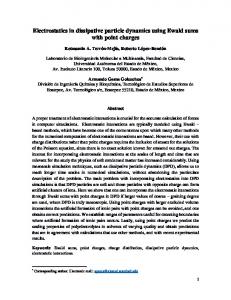
The tracer diffusion of DPD particles has been the subject of various analytical studies. [7, 34, 35, 36] Since this topic is in part related to the present work (see Sect. IV B), we wish to discuss briefly the relevance of usual approximations made in describing the diffusion of DPD particles. The descriptions for tracer diffusion of DPD particles are usually based on a few reasonable approximations. Most importantly, the conservative interactions are typically ignored and the dynamical correlations between particle displace-
ments are neglected. Under these circumstances, the system is described by the Langevin equation (within the Markovian approximation), which yields the tracer diffusion coefficient DT ∼
kB T ∗ . Mγ
(19)
In practice, this expression describes the diffusion of a Brownian particle suspended in liquid. In this context, the absence of conservative interactions is justified since Brownian motion is driven by random forces due to collisions of the Brownian particle with the surrounding fluid particles. Neglecting dynamical correlations is also justified, since Brownian motion is characterized by a random walk in which case the velocity correlation function φ(t) decays exponentially in time, reflecting the lack of memory effects. In models often studied by DPD, the case is rather different, however. First, DPD particles move in the presence of similar particles, and thus consecutive displacements of the tagged particle are likely to be correlated. Second, the conservative interactions are not irrelevant. To clarify this issue, i.e., how well Eq. (19) describes the tracer diffusion of DPD particles, we studied the dependence of DT on the strength of the dissipative force γ. To this end, we investigated models A and B using DPD–VV with a small ∆t (values ranging between 1 × 10⁻³ − 5 × 10⁻³ ). The results are presented in Fig. 9. We find that the behavior of DT in the two models is very different [Fig. 9(a)]. In both cases the power-law dependence DT /hkB T i ∼ (1/γ)x is locally valid, but the exponent x strongly depends on γ and the strength of the conservative force α [see Fig. 9(b)]. In the ideal gas (α = 0) the motion of the DPD particles is fully governed by the random and dissipative forces, and so the exponent x is approximately one at small γ. This behavior is expected, since then the dynamical correlations are very weak, as is confirmed by the exponential decay of φ(t) in this regime (data not shown). This is in agreement with recent results [35, 36] where φ(t) was found to decay exponentially for small friction. At intermediate values of γ, the power-law form of DT is less clear. The exponent x has a minimum around γ = 10, and the velocity correlation function φ(t) decays algebraically rather than exponentially. Finally in the limit of large γ, x tends towards one, which can be understood in terms of a large friction force proportional to M γ, and therefore this regime mimics the diffusion of DPD particles with a large mass. In any case, the decay of φ(t) is not exponential, in agreement with analytical predictions by Espa˜nol and Serrano. [36] In model B with finite conservative interactions, the diffusion at small γ is governed by conservative interactions. This is best demonstrated in Fig. 9(a), where DT is only weakly dependent on γ in the limit of small friction. At intermediate values of γ, there is a crossover regime in which conservative and random forces compete, while at large γ the diffusion behavior becomes dominated by random and dissipative forces. The exponent x varies accordingly, reaching unity only in the limit of large γ. Our aim in this work is not to focus on the diffusion properties of DPD model systems in detail and, thus, we do not con-
10 sider this issue further. Nevertheless, we hope that the present results serve to demonstrate that the dynamics in DPD model systems are not similar to Brownian motion, and this dissimilarity is further enhanced by conservative interactions whose role can be significant. As regards future studies of transport properties of DPD fluid particles, various assumptions made in deriving analytical theories should therefore not be taken for granted.
VI.
SUMMARY AND DISCUSSION
Dissipative particle dynamics (DPD) is a very promising tool for future large-scale simulations of soft systems. Thus far, it has been applied with success to a variety of different problems, including studies of pressure profiles inside lipid bilayers, [10] phase behavior in surfactant solutions, [37] and dynamics of polymer chains. [38] Despite its promising nature, DPD has certain practical problems that have to be accounted for before extensive use in future applications. Many of them are related to the coarse-grained nature of the systems studied. As described by Espa˜nol and Warren, [6] the theoretical framework used in DPD leads to interparticle interactions that include a dissipative term, which depends on the pairwise velocities of DPD particles. This implies that for a proper description of the system in time, the dissipative forces and the particle velocities should be determined hand in hand in a truly self-consistent fashion. As shown in the present work, this issue contains various subtle details, but the key point is that the integration schemes often used in molecular dynamics simulations cannot be used in DPD simulations as such. In this work, we have considered this problem through studies of three different model systems for a number of integration schemes based on the traditional velocity-Verlet approach. We have shown that the traditional velocity-Verlet scheme gives rise to pronounced artifacts in actual physical quantities such as the compressibility and the tracer diffusion coefficient. Further studies presented in this work revealed that the scale of these artifacts can be greatly reduced by accounting for the velocity dependence of dissipative forces. The simplest approach in this regard is to calculate the dissipative forces twice during a single time step, and further improvements can be obtained if the dissipative forces and particle velocities are determined together in a self-consistent fashion through a functional iteration process. For cases where the remaining temperature deviations need to be corrected, we have proposed a self-consistent integrator that is coupled to an auxiliary thermostat. We have discussed its properties through a detailed analysis in two model systems. We have found that this approach works well in the case of equilibrium quantities, whose behavior does not depend on the details of the dynamics. For studies of dynamical quantities such as diffusion, however, care must be taken to avoid misleading interpretations of the data. Problems may appear if hγ(t)i, extracted from simulations with the auxiliary thermostat, deviates significantly from the dissipation strength γ determined by the fluctuation-dissipation theorem. In prac-
tice, this situation is realized if the time step ∆t is relatively large and the role of conservative interactions is weak as compared to random and dissipative forces. However, if care is taken and the auxiliary thermostat is used within proper limits, our results show that it provides an accurate method to study DPD models within the NVT ensemble. The self-consistent integrator with an auxiliary thermostat is an example of a scheme in which the coefficient of the dissipative force is not constant but fluctuates in time. Consequently, the average dissipative force strength hγ(t)i depends on the time increment ∆t. Very recently, den Otter and Clarke suggested another approach, [14, 39] in which the coefficients of the random and dissipative forces depend on the size of the time increment ∆t. The results presented in Ref. 14 indicate that this approach leads to good temperature control [40] compared to the GW scheme, for example, but it remains to be shown through thorough tests if this approach is indeed more successful in minimizing integrator-induced artifacts than the many other schemes suggested previously. As noted in the Introduction, DPD can be thought of as Brownian dynamics with momentum conservation. Both methods are based on coarse graining the underlying microscopic systems, and in both cases the coarse-grained variables are replaced by random noise which is coupled to a dissipative friction term. Consequently, one may question whether similar integrator-induced problems could be faced in Brownian dynamics simulations. While we lack direct evidence, we feel that the problems in Brownian dynamics (if any) are likely less prominent compared to those in DPD. This idea is justified by the fact that in Brownian (Langevin) dynamics, the velocities of tagged particles are coupled to the dissipative force (d~vi / dt ∝ −η ~vi ) individually for every particle. This situation is much easier to deal with compared to that for DPD simulations, where the dissipative term includes contributions from all pairs of particles. A thorough study of this topic would be useful. In the present work we have examined the performance of integration schemes in the well-established description of dissipative particle dynamics, first suggested by Hoogerbrugge and Koelman [5] and later refined by Espa˜nol and Warren. [6] More recently, a number of related schemes have been suggested to shed more light on the underlying structure of DPD, [19] as well as to generalize the framework of DPD for a number of other hydrodynamic cases. [41] These approaches are numerically more complicated than the DPD considered in this work. Studies of the related practical issues would be very interesting, although they are beyond the scope of the present study. We close this work with a brief discussion of the situations, in which DPD-specific artifacts due to integration schemes are expected. To this end, we first summarize our main findings. We have noticed in all three model systems that various integrators lead to pronounced artifacts in DPD model systems, if random and dissipative interactions are strong compared to conservative interactions. On the other hand, if the system is governed by conservative interactions, then the artifacts have been found to be weaker. This suggests that one should use conservative interactions that are sufficiently strong to dom-
11 inate the behavior of the model system, and let random and dissipative forces act only as a thermostat. Although this arrangement with dominating conservative forces is feasible in a number of cases, [42, 43] there are also many systems studied by DPD where random and dissipative forces are rather weak but comparable to conservative interactions. Furthermore there are processes governed by collective effects at large particle densities in the high friction limit, which based on our work can lead to integrator-induced artifacts. Moreover, future aims to examine soft systems of biological molecules in an explicit solvent lead naturally to studies of hybrid models, where a microscopic description for biomolecules is combined with a coarse-grained description for the solvent. In these cases there are both strong conservative interactions and relatively weak soft interactions, where soft interactions for the solvent are still subject to integrator-
induced artifacts, and may affect the behavior of the system as whole. The overall picture of the role of integration schemes in specific model systems is therefore still incomplete, and more work is required to resolve these issues. [44] Meanwhile, we emphasize that the artifacts are related to the dissipative force term, and therefore care should be taken in all cases where this term plays an important role.
[1] D. Frenkel and B. Smit, Understanding Molecular Simulation: From Algorithms to Applications (Academic Press, San Diego, 1996). [2] A. J. C. Ladd, Phys. Rev. Lett. 70, 1339 (1993); J. Fluid Mech. 271, 285 (1994); J. Fluid Mech. 271, 311 (1994). [3] M. Murat and K. Kremer, J. Chem. Phys. 108, 4340 (1998). [4] A. Malevanets and R. Kapral, J. Chem. Phys. 110, 8605 (1999); J. Chem. Phys. 112, 7260 (2000). [5] P. J. Hoogerbrugge and J. M. V. A. Koelman, Europhys. Lett. 19, 155 (1992). [6] P. Espa˜nol and P. Warren, Europhys. Lett. 30, 191 (1995). [7] R. D. Groot and P. B. Warren, J. Chem. Phys. 107, 4423 (1997). [8] P. B. Warren, Curr. Opin. Colloid. Interf. Sci. 3, 620 (1998). [9] R. D. Groot, T. J. Madden, and D. J. Tildesley, J. Chem. Phys. 110, 9739 (1999). [10] M. Venturoli and B. Smit, PhysChemComm 10 (article 10) (1999). [11] K. E. Novik and P. V. Coveney, J. Chem. Phys. 109, 7667 (1998). [12] I. Pagonabarraga, M. H. J. Hagen, and D. Frenkel, Europhys. Lett. 42, 377 (1998). [13] J. B. Gibson, K. Chen, and S. Chynoweth, Int. J. Mod. Phys. C 10, 241 (1999). [14] W. K. den Otter and J. H. R. Clarke, Europhys. Lett. 53, 426 (2001). [15] P. Ahlrichs and B. D¨unweg, J. Chem. Phys. 111, 8225 (1999). [16] A. Malevanets and J. Yeomans, Europhys. Lett. 52, 231 (2000). [17] G. Besold, I. Vattulainen, M. Karttunen, and J. M. Polson, Phys. Rev. E 62, R7611 (2000). [18] B. M. Forrest and U. W. Suter, J. Chem. Phys. 102, 7256 (1995). [19] E. G. Flekkøy and P. V. Coveney, Phys. Rev. Lett. 83, 1775 (1999); E. G. Flekkøy, P. V. Coveney, and G. De Fabritiis, Phys. Rev. E 62, 2140 (2000). [20] C. W. Gardiner, Handbook of Stochastic Methods (SpringerVerlag, Berlin, 1983). [21] B. D¨unweg and W. Paul, Int. J. Mod. Phys. C, 2, 817 (1991). [22] P. L’Ecuyer, Commun. ACM 31, 742 (1988). [23] W. H. Press, S. A. Teukolsky, W. T. Vetterling, B. P. Flannery, Numerical Recipes in Fortran, The Art of Scientific Computing, 2nd Edition (Cambridge University Press, Cambridge, 1992) pp. 271–273. [24] I. Vattulainen, submitted (2001).
[25] M. E. Tuckerman and G. J. Martyna, J. Phys. Chem. B 104, 159 (2000). [26] L. Verlet, Phys. Rev. 159, 98 (1967). [27] M. P. Allen and D. J. Tildesley, Computer Simulation of Liquids (Oxford University Press, Oxford, 1993). [28] G. J. Martyna and M. E. Tuckerman, J. Chem. Phys. 102, 8071 (1995). [29] J. M. Thijssen, Computational Physics (Cambridge University Press, Cambridge, 1999). [30] J. P. Boon and S. Yip, Molecular Hydrodynamics (Dover, New York, 1980). [31] For ∆t > ∼ 0.1, the positive and negative deviations from g(r) = 1 accidentally almost cancel each other. [32] J.-P. Hansen and I. R. McDonald, Theory of Simple Liquids, 2nd edition (Academic Press, San Diego, 1986). [33] Th. Soddemann, B. D¨unweg, and K. Kremer (unpublished). [34] C. A. Marsh, G. Backx, and M. H. Ernst, Europhys. Lett. 38, 411 (1997); Phys. Rev. E 56, 1676 (1997). [35] A. J. Masters and P. B. Warren, Europhys. Lett. 48, 1 (1999). [36] P. Espa˜nol and M. Serrano, Phys. Rev. E 59, 6340 (1999). [37] J. C. Shelley and M. Y. Shelley, Curr. Opin. Colloid Interface Sci. 5, 101 (2000). [38] N. A. Spenley, Europhys. Lett. 49, 534 (2000). [39] W. K. den Otter and J. H. R. Clarke, Int. J. Mod. Phys. C 11, 1179 (2000). [40] Den Otter and Clarke have pointed out that there is no unique way to define the temperature of the system, [14, 39] and that the different definitions (in terms of the kinetic energy or the configurational temperature, for example) may not be completely consistent in the context of DPD. ¨ [41] P. Espa˜nol, M. Serrano, and H. C. Ottinger, Phys. Rev. Lett. 83, 4542 (1999); M. Serrano and P. Espa˜nol, Phys. Rev. E 64, 046115 (2001). [42] W. Dzwinel and D. A. Yuen, J. Colloid Interface Sci. 225, 179 (2000). [43] W. Dzwinel and D. A. Yuen, Int. J. Mod. Phys. C 11, 1 (2000). [44] P. Nikunen, M. Karttunen, and I. Vattulainen (unpublished).
Acknowledgements — This work has, in part, been supported by the Academy of Finland through its Centre of Excellence Program (I.V. and M.K.), and by a grant from the European Union (I.V.). Further support from the Alfred Kordelin Foundation and the Jenny and Antti Wihuri Foundation is greatly acknowledged (I.V.).
12
F~iC {~rj },
(4) ~vi ←− ~vi + (5) Calculate b
(s) Calculate a with
step [calculation of temperature kB T , g(r), . . . ]
MD-VV GW SC-Th DPD-VV GCC SC-VV
1.20 1.10 1.00 0.90
(2) ~ri ←− ~ri + ~vi ∆t (3) Calculate
b Sampling
< kB T >
TABLE I: Update scheme for a single integration step (time increment ∆t) for various integration schemes in DPD (for acronyms see text). For positions and velocities at time t, the updated positions and velocities at time t + ∆t are given by the corresponding variables on the right-hand side of steps (2) and (4) below, respectively. GW(λ) : steps (0)–(4), (s) MD–VV ≡ GW(λ = 1/2) : steps (1)–(4), (s) a GCC(λ) : steps (0)–(5), (s) DPD–VV ≡ GCC(λ = 1/2) : steps (1)–(5), (s) a √ � 1 � ~C ~iD ∆t + F ~iR ∆t (0) ~vi◦ ←− ~vi + λ Fi ∆t + F m √ � 1 1 �~C ~iD ∆t + F~iR ∆t Fi ∆t + F (1) ~vi ←− ~vi + 2 m
F~iD {~rj , ~vj◦ },
~iR {~rj } F
√ � 1 1 �~C ~iD ∆t + F~iR ∆t Fi ∆t + F 2 m
F~iD {~rj , ~vj }
N m X 2 kB T = ~v , 3N −3 i=1 i
substitution of ~vj for ~ vj◦ in step (3).
...
10
-2
10
-1
t FIG. 1: Results for the deviations of the observed temperature hkB T i from the desired temperature kB T ∗ ≡ 1 vs. the size of the time step ∆t in model A. Results of GW and GCC are for λ = 0.65.
13 TABLE II: Update scheme for the two self-consistent integrators without (SC–VV) and with (SC–Th) the auxiliary thermostat [steps (i)–(iii)]. The self-consistency loop is over steps (4b) and (5) as indicated. For positions and velocities at time t, the updated positions and velocities at time t + ∆t are given by the corresponding variables on the right-hand side of steps (2) and (4b) below (after the last iteration of the self-consistency loop), respectively. The desired temperature is kB T ∗ . Initialization: η = 0, γ = σ 2 /(2kB T ∗ ), and kB T is calculated from the initial velocity distribution. (i)
η˙
(ii) η
←− C (kB T − kB T ∗ ) ←− η + η˙ ∆t
σ2 (1 + η ∆t) 2 kB T ∗ √ � 1 1 �~C ~iD ∆t + F~iR ∆t Fi ∆t + F (1) ~vi ←− ~vi + 2 m (iii) γ ←−
(2) ~ri ←− ~ri + ~vi ∆t (3) Calculate
F~iC {~rj },
F~iD {~rj , ~vj },
~iR {~rj } F √ o 1 n~C ~iR ∆t Fi ∆t + F m 1 ~D F ∆t m i
1 b (4a) ~ v i ←− ~vi + 2 - (4b) ~vi ←− ~bv i + 1 2 D (5) Calculate F~i {~rj , ~vj } (s)
Calculate
kB T =
N m X 2 ~v , 3N −3 i=1 i
...
1.15 MD-VV DPD-VV SC-VV
g(r)
1.10 1.05
t = 0.010
t = 0.050
t = 0.100
t = 0.200
1.00 0.95 1.15
g(r)
1.10 1.05 1.00 0.95 0.0
0.5
r / rc
1.0 0.0
0.5
1.0
r / rc
FIG. 2: Radial distribution functions g(r) vs. ∆t in model A for the integration schemes MD–VV, DPD–VV, and SC–VV. Results of GW and GCC are almost similar to MD–VV and DPD–VV, respectively, and are therefore omitted here.
14
0.58
1.000 0.950 (a)
(b)
0.56
T
DT
0.900 0.850
0.54
0.800 SC-VV DPD-VV MD-VV
0.750
0.52 -2
10
10
-1
-2
10
t
10
-1
t
SC-VV SC-Th DPD-VV MD-VV
4.0
-2
10
t
10
1.8
-1
1.6
0.60 (a)
(b)
1.4
0.55
10
-2
-1
10
t
-2
10
10
DT
0.72
DT
0.65
4.5
< (t) >
0.70
/ < kB T >
FIG. 3: (a) The relative isothermal compressibilities e κT vs. ∆t evaluated from g(r) in model A. Ideally one would obtain κ eT = 1, and the deviations from this limit reflect artifacts due to the integration procedure. (b) Results for the tracer diffusion coefficient DT vs. the time step ∆t in model A.
-1
t
FIG. 4: (a) Results for the tracer diffusion coefficient DT vs. ∆t in model A for the SC–Th integrator, in which γ is not fixed but fluctuates in time. Results of DPD–VV are also given for the purpose of comparison. The inset illustrates the dependence of hγ(t)i on ∆t for the SC–Th integration scheme. (b) The scaled tracer diffusion coefficient DT γ x /hkB T i with x = 0.72.
15
MD-VV DPD-VV SC-Th GW GCC SC-VV
< kB T >
1.04 1.02 1.00 0.98
-2
-1
10
10
t FIG. 5: Results for the deviations of the observed temperature hkB T i from the desired temperature kB T ∗ = 1 vs. the size of the time step ∆t in model B. Results of GW and GCC are for λ = 0.65.
0.30
< (t) >
4.65 4.50 4.35
-2
10
0.06
0.29
-1
t
10
DT
T
0.07
4.80
MD-VV SC-Th DPD-VV GW GCC SC-VV
0.28 0.05 (a) -2
10
10
t
0.27
(b) -1
-2
-1
10
10
t
FIG. 6: (a) The relative isothermal compressibilities κ eT evaluated from g(r) in model B. (b) Results for the tracer diffusion coefficient DT vs. ∆t in model B. Results of GW and GCC are for λ = 0.65. The inset illustrates the dependence of hγ(t)i on ∆t for the SC– Th integration scheme as compared to γ = 4.5 determined by the fluctuation-dissipation theorem.
16
2.5
= 0.7 = 0.1
g(r)
2.0 1.5 1.0 0.5 0.0
0.0 0.5 1.0 1.5 2.0 2.5
r / rc FIG. 7: Results for g(r) in model C with σ = 1 using the integrators MD–VV and DPD–VV. Results are shown for the density ρ = 0.1 with ∆t = 0.01, and for the density ρ = 0.7 with ∆t = 0.001. The results of DPD–VV and MD–VV are essentially identical.
MD-VV DPD-VV MD-VV DPD-VV
0.14
(a)
1.02
0.13
(b)
0.12
100
1.00
D
F
F(r)
< kB T >
1.03
0.99
F
C
0.11
R
F
0.98
0 0.0 0.4 0.8 1.2
t = 0.01 t = 0.001
0
100
0.10
r / rc
200 0
DT
1.04
100
200
FIG. 8: Results for (a) the temperature hkB T i and (b) the tracer diffusion coefficient DT vs. the strength of the random force σ in model C with ρ = 0.7. Results are shown for the integration schemes MD–VV and DPD–VV with two different time steps. For ∆t = 0.01 with MD–VV, the system no longer remained stable beyond σ = 50. To clarify the crossover from the regime dominated by conservative interactions to the regime dominated by random and dissipative forces, we have shown in the inset of (b) the interactions F R (dot-dashed), F D (dashed), and F C (full line) for σ = 60. For σ > 60, the dissipative force is steeper than the conservative one.
17
no. of iterations nit
50
2.5 2.0
-4
| ∆T/T | < 10
-6
1.5
| ∆T/T | < 10
tCPU(nit) tCPU(0)
10 5
0.11 0.12
1.0
1 0.01
∆t
0.05
0.10
FIG. 9: Computational efficiency of the self-consistent integration scheme SC–VV via functional iteration. Shown here is the average number of iterations nit as a function of the employed time step ∆t to obtain the desired accuracy. The accuracy is described by the Figure 9 by Vattulainen et al. modulus of ∆T /T of the instantaneous temperature, and results are shown for ∆T /T < 10−6 (solid diamonds) and ∆T /T < 10−4 (solid circles). The corresponding CPU time relative to the CPU time for plain DPD–VV (“0 iterations”) is also shown.
1.0 (a)
(b)
DT / < kBT >
0.8
10
0
0.6
x
10
0.4 0.2
-1 =0 = 25
0.0 10
0
10
1
10
2
10
0
1
10
10
2
FIG. 10: (a) Diffusion results for DT /hkB T i vs. the strength of the dissipative force γ in DPD simulations for models A (α = 0) and B (α = 25). (b) Based on the results in (a) and using the ansatz DT /hkB T i ∼ γ −x , here is shown the resulting exponent x as a function of γ. The results shown here have been calculated by DPD– VV with small ∆t (ranging from 1 × 10⁻³ to 5 × 10⁻³ ) such that temperature deviations in all cases are very minor.