Jun 9, 2005 - well advanced in years, by no means out-dated. ... theoretical predictions for the ideal dissipative fluid, I have applied ..... The solutions of the Navier-Stokes equation (2.38) have to be ...... An if-instruction around the whole warm-up checks whether this ..... fα = hkâr2 ...... #package require math::constants.
Dissipative Particle Dynamics A Study of the Methodological Background
Ulf Daniel Schiller
9th June 2005
Diploma Thesis
Supervised by Prof. Dr. Friederike Schmid Condensed Matter Theory Group Faculty of Physics University of Bielefeld
Thus natural science appears completely to lose from sight the large and general questions; but all the more splendid is the success when, groping in the thicket of special questions, we suddenly find a small opening that allows a hitherto undreamt of outlook on the whole. L UDWIG B OLTZMANN
Contents
1 Introduction 2 Theoretical Foundations 2.1 Classical Mechanics . . . . . . . . . . . . . . . . . . . . . . . 2.1.1 Liouville Formulation of Classical Mechanics . . . . . 2.2 Statistical Mechanics and Thermodynamics . . . . . . . . . . 2.2.1 Ensembles, Ergodicity, Averages, Partition Function . 2.2.2 Thermodynamics . . . . . . . . . . . . . . . . . . . . 2.3 Hydrodynamics . . . . . . . . . . . . . . . . . . . . . . . . . 2.3.1 Continuum Mechanics . . . . . . . . . . . . . . . . . 2.3.2 Kinetic Theory . . . . . . . . . . . . . . . . . . . . . 2.4 Computer Simulations . . . . . . . . . . . . . . . . . . . . . 2.4.1 Molecular Dynamics . . . . . . . . . . . . . . . . . . 2.4.2 Liouville Formulation of the Velocity-Verlet Algorithm 2.4.3 Langevin Dynamics . . . . . . . . . . . . . . . . . . 2.5 Measurements in Computer Simulations . . . . . . . . . . . . 2.5.1 Averages and Errors . . . . . . . . . . . . . . . . . . 2.5.2 Thermodynamic Properties . . . . . . . . . . . . . . . 2.5.3 Structural Properties . . . . . . . . . . . . . . . . . . 2.5.4 Correlation Functions . . . . . . . . . . . . . . . . . 2.5.5 Transport Coefficients . . . . . . . . . . . . . . . . . 2.5.6 Local Observables . . . . . . . . . . . . . . . . . . . 2.6 Coarse-Graining . . . . . . . . . . . . . . . . . . . . . . . . . 2.6.1 Levels of Description . . . . . . . . . . . . . . . . . . 2.6.2 Theory of Coarse Graining . . . . . . . . . . . . . . . 2.6.3 The GENERIC Structure . . . . . . . . . . . . . . . .
1
. . . . . . . . . . . . . . . . . . . . . . .
. . . . . . . . . . . . . . . . . . . . . . .
. . . . . . . . . . . . . . . . . . . . . . .
. . . . . . . . . . . . . . . . . . . . . . .
. . . . . . . . . . . . . . . . . . . . . . .
3 Dissipative Particle Dynamics 3.1 A Short History of Dissipative Particle Dynamics . . . . . . . . . . . . 3.2 Dissipative Particle Dynamics . . . . . . . . . . . . . . . . . . . . . . 3.3 Stochastic Differential Equations and Fokker-Planck Equations for DPD 3.4 H-Theorems for DPD . . . . . . . . . . . . . . . . . . . . . . . . . . . 3.5 Hydrodynamics for DPD . . . . . . . . . . . . . . . . . . . . . . . . . 3.6 DPD with Finite Time Step . . . . . . . . . . . . . . . . . . . . . . . . 3.7 Energy Conserving DPD . . . . . . . . . . . . . . . . . . . . . . . . . 3.8 Microscopic Foundations of DPD . . . . . . . . . . . . . . . . . . . . 3.8.1 Voronoi Fluid Particles . . . . . . . . . . . . . . . . . . . . . . 3.8.2 Soft Fluid Particles . . . . . . . . . . . . . . . . . . . . . . . .
. . . . . . . . . . . . . . . . . . . . . . .
. . . . . . . . . .
. . . . . . . . . . . . . . . . . . . . . . .
. . . . . . . . . .
. . . . . . . . . . . . . . . . . . . . . . .
. . . . . . . . . .
. . . . . . . . . . . . . . . . . . . . . . .
. . . . . . . . . .
. . . . . . . . . . . . . . . . . . . . . . .
4 4 5 6 6 7 8 8 12 16 17 20 21 24 24 25 26 27 27 28 31 31 32 36
. . . . . . . . . .
39 41 45 48 51 53 56 59 62 63 70
iii
Contents 3.9 The Theory of Marsh, Backx and Ernst . . . . . . . . . . . . . . . . . . . . . . . 3.10 Boltzmann Theory for Dissipative Particle Dynamics . . . . . . . . . . . . . . .
74 80
4 The ESPResSo-Package and Extensions 4.1 ESPResSo - Extensible Software Package for Research on Soft Matter 4.1.1 General Parameters . . . . . . . . . . . . . . . . . . . . . . . . 4.1.2 Particles . . . . . . . . . . . . . . . . . . . . . . . . . . . . . . 4.1.3 Interactions . . . . . . . . . . . . . . . . . . . . . . . . . . . . 4.1.4 Force Calculation . . . . . . . . . . . . . . . . . . . . . . . . . 4.1.5 Integration . . . . . . . . . . . . . . . . . . . . . . . . . . . . 4.1.6 Constraints . . . . . . . . . . . . . . . . . . . . . . . . . . . . 4.1.7 Thermostats . . . . . . . . . . . . . . . . . . . . . . . . . . . . 4.1.8 Periodic Boundary Conditions . . . . . . . . . . . . . . . . . . 4.1.9 Verlet Lists and Cell Lists . . . . . . . . . . . . . . . . . . . . 4.1.10 Parallelization . . . . . . . . . . . . . . . . . . . . . . . . . . 4.1.11 Reentering the Integrator . . . . . . . . . . . . . . . . . . . . . 4.2 How to Set Up a Simulation with ESPResSo . . . . . . . . . . . . . . 4.2.1 Setting Parameters . . . . . . . . . . . . . . . . . . . . . . . . 4.2.2 System Setup . . . . . . . . . . . . . . . . . . . . . . . . . . . 4.2.3 Warm-Up Integration and Equilibration . . . . . . . . . . . . . 4.2.4 Integration and Measurements . . . . . . . . . . . . . . . . . . 4.3 Extensions to ESPResSo . . . . . . . . . . . . . . . . . . . . . . . . 4.3.1 Local Observables . . . . . . . . . . . . . . . . . . . . . . . . 4.3.2 Local Volume of Global Constraints . . . . . . . . . . . . . . .
. . . . . . . . . . . . . . . . . . . .
. . . . . . . . . . . . . . . . . . . .
. . . . . . . . . . . . . . . . . . . .
. . . . . . . . . . . . . . . . . . . .
. . . . . . . . . . . . . . . . . . . .
84 85 86 86 87 89 91 92 94 95 96 98 100 102 102 103 104 105 108 108 111
5 Case Studies with Dissipative Particle Dynamics 5.1 Simulation of an Ideal Dissipative Fluid . . . . . . 5.1.1 Simulation Setup . . . . . . . . . . . . . . 5.1.2 Simulation Results . . . . . . . . . . . . . 5.1.3 Discussion of Results . . . . . . . . . . . . 5.2 Simulation of Stokes Flow around a Sphere . . . . 5.2.1 Simulation Setup . . . . . . . . . . . . . . 5.2.2 Simulation Results . . . . . . . . . . . . . 5.2.3 Summary and Discussion of Results . . . .
. . . . . . . .
. . . . . . . .
. . . . . . . .
. . . . . . . .
. . . . . . . .
114 114 115 116 125 129 129 129 139
. . . . . . . .
. . . . . . . .
. . . . . . . .
. . . . . . . .
. . . . . . . .
. . . . . . . .
. . . . . . . .
. . . . . . . .
. . . . . . . .
. . . . . . . .
. . . . . . . .
6 Summary and Outlook
142
Acknowledgments
145
A Source Code A.1 Simulation of the Ideal Dissipative Fluid . . . A.2 Simulation of Stokes Flow around a Sphere . A.3 Monte-Carlo Integration of Collision Integrals A.4 Pressure Correlation Function . . . . . . . . A.5 Local Observables in ESPResSo . . . . . . A.6 Local Subvolumes of a Sphere . . . . . . . .
147 148 153 159 163 165 172
Bibliography
iv
. . . . . .
. . . . . .
. . . . . .
. . . . . .
. . . . . .
. . . . . .
. . . . . .
. . . . . .
. . . . . .
. . . . . .
. . . . . .
. . . . . .
. . . . . .
. . . . . .
. . . . . .
. . . . . .
. . . . . .
. . . . . .
. . . . . .
175
1 Introduction Computer simulations have beyond doubt become one of the most important research tools in modern physics. The reason for this is the fact that our theoretical description of nature is expressed in mathematical equations, which only in a few exceptional cases can be solved exactly. This holds true even for relatively simple theories, such as Newtonian mechanics, where already the motion of three interacting bodies cannot be predicted in terms of an analytical solution. Hence in the majority of non-trivial cases, we have to resort to approximations in order to obtain predictions from the theoretical models. Such approximations may be either analytical or numerical in nature. While theories are the basis for comprehending nature, experiments provide the observations that are to be comprehended. Therefore, it is essential to compare the theoretical predictions against the experimental results in order to verify the validity of the theoretical models. At this point, approximate theories impose difficulties: The concrete effects of the approximation are often uncontrollable, such that in case of significant deviations between theory and experiment it is difficult to assess whether they are caused by the approximations or not. This means that the verification of approximate theories against the experimental observations is rather unreliable. Computer simulations serve as a bridge between theory and experiment. With the advent of digital computers it became possible to solve complex problems without having to rely on approximations. This is achieved by the powerful calculational capabilities of the computer, which enable us to obtain solutions that are – apart from numerical and discretization errors – exact results. These exact results can be compared with the predictions of approximate theories and thus serve as a test of theories. The other way round, results of a computer simulation can be compared with experimental measurements and thus serve as a test of models. In this way, the comparison of theory and experiment becomes more conclusive because the origin of discrepancies can now explicitly be assigned to the approximations or to the model itself. Another aspect of simulations, which maybe is more pronounced today, is to view them as computer experiments. A computer simulation provides the connection between the microscopic details of a model and the macroscopic properties of interest, that is, the observables being measured in an according experiment. Sometimes it may be difficult or even impossible to obtain measurements from an experimental setup, for example under extreme conditions like high temperature or high pressure. Then the computer can function as a virtual ‘laboratory’, where perfect control of all parameters is possible and accurate ‘measurements’ can be acquired. It is hence possible to probe the properties of interest for a theoretical model in great detail, which in turn can lead to a better understanding of the theory. Moreover, a computer simulation allows to explore how the microscopic structure is related to the bulk properties. This is possible by switching on or off the different features of the model and study the effects separately. In doing so, one can identify the contributing factors that are responsible for the emergence of collective phenomena. There are many examples where computer simulations have helped in elucidating the physical mechanisms of a complex system, and the construction of new hypothetical models is today inextricably linked
1
1 Introduction to their exploration by means of computer simulation. To summarize the role of computer simulation, I adopt the view of Landau and Binder [2000] here, where theory, experiment and simulation are depicted as three vertices of a triangle surrounding our understanding of nature. There is a vast number of application fields for computer simulations. Generally, they can be used to study the equilibrium and non-equilibrium properties of solids, fluids and gases. More concrete examples, where computer simulations are applied, are phase-transitions and critical phenomena, the properties of liquid crystals and the study of biomolecules like proteins or DNA. Maybe the most challenging application of computer simulations are fluid systems, as the structure and dynamics of complex fluids still comprises many phenomena which are not well understood. This ranges from colloidal systems over fluid dynamics and rheology to biological systems like membranes and finally living cells. Today a variety of simulation methods exists, and strictly speaking, the term computer simulation is ambiguous. The first simulation method came up over 50 years ago, when in March 1952 the Los Alamos computer MANIAC was put into operation. It is the famous Monte Carlo (MC) method, which uses random numbers to sample the phase space of a given system in order to evaluate statistical observables in terms of phase-space integrals. Since in the Monte Carlo method, the momentum part of the phase space has been integrated out, no ‘real’ dynamics can be simulated. However, MC is very successful in simulating systems at equilibrium and the method is, though well advanced in years, by no means out-dated. A method to simulate the dynamic properties of a system was first used in the late 1950s. The Molecular Dynamics (MD) method solves Newton’s equations of motion and obtains the trajectory of the system in discrete time steps. Many refinements to the MD method have been developed over the years, but as with MC, the basic MD algorithm is today still effectively used. Monte Carlo and Molecular Dynamics are only the two most basic simulation techniques. Many sophisticated refinements and extensions have been developed for various contexts. Although computer facilities have been subject to rapid improvement since the pioneering simulations, machine performance still sets limitations in terms of CPU time and memory requirements. This primarily restricts the size of the system that can be simulated, e.g. the number of particles that can be handled with the given resources. In this sense, fluid systems are especially demanding because the solvent has to be represented by a large number of molecules. Furthermore, the interesting phenomena in complex fluids appear on time scales much larger than the motion of the individual solvent particles. Therefore in a conventional MD simulation, a great deal of computing time is used for rather uninteresting behavior. As a consequence, there still are problems for which a simulation turns out to be inefficient or even intractable. Fortunately, there exist strategies to overcome these limitations. They aim at reducing the number of degrees of freedom by representing the system through a set of relevant variables that evolve on a more suitable time scale. The general procedure to remove ‘uninteresting’ degrees of freedom is called coarse-graining. One such approach is known as Brownian dynamics and is based on the Langevin equations. Like MD, it is a continuum-dynamical method, but the forces have a stochastic part that models a fluctuating environment, e.g. a solvent. The attempt to reduce computational costs also led to the invention of lattice-based algorithms, many of which are based on cellular automata. These methods, such as the lattice gas (LG) or lattice Boltzmann (LB) approach, rely on a spatial discretization of the system. They are quite efficient but also introduce some conceptual difficulties. The stochastic forces of Brownian dynamics are not momentum conserving, and the lattice-based
2
methods violate Galilean invariance. Consequently one may argue that these methods are not the best choice for the simulation of fluid dynamics. In this thesis, I study Dissipative Particle Dynamics (DPD), a method invented for carrying out particle based simulations of hydrodynamic behavior. DPD combines ideas from Langevin dynamics and lattice gas algorithms. The according equations are constructed such that Galilean invariance and momentum conservation are fulfilled. Hence the method is expected to produce correct hydrodynamic behavior. The aim of this thesis is to give a survey of the DPD method, to review the theoretical background and to explore its practical applicability. The itinerary of this work is organized as follows: In chapter 2, I provide the theoretical foundations that are used in this work. The material is meant to give a self-contained introduction of the necessary concepts and shall make the reader familiar with the notation. The Dissipative Particle Dynamics method is introduced in chapter 3. I give a review of the basic technique and a survey of important theoretical aspects. Further, I present the extension to energy conserving DPD, and I discuss the microscopic foundations with respect to the theory of coarse-graining. The chapter is closed with a presentation of two different theories for deriving the transport properties of the ideal DPD fluid. Chapter 4 contains the part of this work that deals with programming. I sketch the basic techniques for implementing a computer simulation considering as example the ESPResSo software package. I also explain how a concrete simulation can be carried out with ESPResSo. In addition, I describe the new extensions that have been implemented during this work. In chapter 5, I carry out two case studies with dissipative particle dynamics. These shall demonstrate how the method works and how the results can be interpreted. Besides having tested some theoretical predictions for the ideal dissipative fluid, I have applied the method to a concrete hydrodynamic problem, namely Stokes flow around a sphere. I give a summary of the different aspects of DPD in chapter 6 and sketch some perspectives for future research with the dissipative particle dynamics method.
3
2 Theoretical Foundations This chapter gives a brief introduction into the theoretical concepts that are used in this work. Due to the broad range of aspects that are related to the topic it is not possible to cover all of them exhaustively. However, I try to present an overview of the foundations that is as much selfcontained as possible in the present scope. At first, I review the foundations of classical mechanics, hydrodynamics and thermodynamics. Then I outline the basics of computer simulation techniques, particularly Molecular Dynamics and Langevin Dynamics. I close the chapter with a sketch of the theory of coarse-graining.
2.1 Classical Mechanics The methodology of this work is based on the laws of ‘classical’ physics, i.e. neither relativistic nor quantum effects will be taken into account. For the systems under consideration this means that the velocity of particles is assumed to be small compared to the speed of light, and the frequency ν is assumed to satisfy hν < kB T . These assumptions are very well justified for many materials [cf. Frenkel and Smit, 1996]. In classical (Hamiltonian) mechanics, the time evolution of a system of particles is given by the Lagrangian equation of motion1 � � ∂L d ∂L − = 0, (2.1) dt ∂ q˙i ∂qi where qi and q˙i are generalized coordinates and velocities, respectively [Goldstein, 1991]. The ˙ given in terms of the kinetic energy K and the potential V : Lagrangian L is a function of (q, q), L = K − V.
(2.2)
Using Cartesian coordinates ri and the usual definition of the kinetic energy K=
1X mi r˙ 2i 2
(2.3)
i
and forces fi fi = ∇ri L = −∇ri V,
(2.4)
the Euler-Lagrange equation (2.1) yields Newton’s equation of motion mi ¨ri − fi = 0. 1
4
(2.5)
There exist several equivalent formalisms in classical mechanics, and it is a matter of taste which one prefers. The Lagrangian formulation is perhaps more suited for extensions to field theories, where a corresponding Euler-Lagrange equation can be formulated in terms of a Lagrangian density L.
2.1 Classical Mechanics Introducing generalized momenta p i conjugate to the coordinates pi =
∂L , ∂ q˙i
we can define the Hamiltonian for the system X H= q˙i pi − L.
(2.6)
(2.7)
i
If the potential does not depend on the velocities q˙ i and the time t, the Hamiltonian resembles the energy [Goldstein, 1991]. The Hamiltonian equations of motion are ∂H , ∂pi ∂H p˙ i = − . ∂qi
(2.8)
pi , mi p˙ i = fi .
(2.9)
q˙i =
For cartesian coordinates we get r˙ i =
While (2.5) is a system of 3N second-order differential equations, (2.9) is a system of 6N first order differential equations. Both systems are equivalent but they can lead to different discrete algorithms for their solution. The Euler algorithm introduced in section (2.4.1) uses the first order system while the Verlet algorithm uses the second order system.
2.1.1 Liouville Formulation of Classical Mechanics All positions and momenta together form the phase-space Γ = {r i , pi }, which contains all information about the microscopic state of the system. A trajectory in this phase-space is denoted by Γ(t), and the density distribution in phase-space is denoted by ρ(Γ; t). For an arbitrary function A(Γ) in phase-space (e.g. an observable), the time evolution can be derived from the equations of motion (2.9) � X � ∂A ∂A d (2.10) r˙ i + p˙ i = iLA(Γ), A(Γ) = dt ∂ri ∂pi i
where we have introduced the Liouville operator � X� ∂ ∂ + p˙ i r˙ i iL = . ∂ri ∂pi
(2.11)
i
From the equations of motion follows Liouville’s theorem: ∇Γ Γ˙ = 0. It implies the continuity equation for the phase-space density � � ∂ρ + ∇Γ ρΓ˙ = 0. ∂t
(2.12)
(2.13)
5
2 Theoretical Foundations As a consequence, the phase-space density along a trajectory is conserved d ρ(Γ; t) = 0, dt
(2.14)
and application of the chain rule yields Liouville’s equation ∂ ρ(Γ; t) + iLρ(Γ; t) = 0 ∂t
(2.15)
The Liouville formulation can be used to derive symplectic algorithms for Molecular Dynamics.
2.2 Statistical Mechanics and Thermodynamics In complex systems there are usually very many particles. Such systems are better described by their macroscopic properties like temperature, pressure etc., than by every single trajectory of the constituting particles. The description of systems in terms of macroscopic parameters is the field of thermodynamics. Historically, thermodynamics is a phenomenological theory, which is directly based on experimental observations. It is founded on intuitive postulates and many concepts have been developed, for example the equations of state, thermodynamic transformations, etc. [Huang, 1987]. The First Law of Thermodynamics was formulated by ROBERT M AYER in 1842. The Second Law of Thermodynamics was stated in 1850 by W. T HOMSON, later known as L ORD K ELVIN. Statistical Mechanics puts thermodynamics on a microscopic basis and explains the macroscopic observations by the molecular motion of the system. In this sense, the macroscopic parameters are statistical averages of microscopic properties. In this section, I will sketch the basics of statistical mechanics and thermodynamics.
2.2.1 Ensembles, Ergodicity, Averages, Partition Function A system is described by the positions and momenta of all particles in the 6N -dimensional phase space Γ = (rN , pN ). These microscopic degrees of freedom evolve according to the equations of classical mechanics (cf. section 2.1). However, since we are interested in macroscopic parameters only, it does not matter in which microscopic state the system is, as long as it gives rise to the correct macroscopic values. This will usually be a whole set of systems, which is called an ensemble. The distribution of the systems in phase space is given by the phase space density ρ(Γ; t). Usually, one makes the (quasi-)ergodic assumption, which states that the system will come arbitrarily close to any point in the accessible phase space, i.e. almost every trajectory will cover almost the entire accessible phase space. If a system is (quasi-)ergodic, time averages can be replaced by ensemble averages: Z Z 1 T dΓ ρ(Γ) A(Γ). (2.16) dt A(Γ) = lim T →∞ T 0 Ω To obtain the phase-space densities ρ(Γ; t), one often makes another postulate 2 : The postulate of equal a priori probability or maximal ignorance. With the phase-space densities, one can finally 2
6
Strictly speaking, this postulate is not necessary. However, it simplifies the treatment considerably.
2.2 Statistical Mechanics and Thermodynamics write down the ensemble average of an observable A(Γ): Z dΓ ρ(Γ) A(Γ). hAi =
(2.17)
Ω
It is convenient to introduce the partition function that contains all necessary information about the system. In the canonical ensemble it is Z 1 ZK = dΓ exp (−βH(Γ)) , (2.18) N ! h3N Ω where H(Γ) is the Hamiltonian of the System, h is a constant to make Z dimensionless, and the inverse temperature β is (kB is the Boltzmann constant) β=
1 . kB T
With the partition function we can rewrite the average of equation (2.17): Z 1 hAi = dΓ A(Γ) exp (−βH(Γ)) . ZK Ω
(2.19)
(2.20)
2.2.2 Thermodynamics From the point of view of thermodynamics, all information about the system is contained in the thermodynamic potential. The thermodynamic potentials for different ensembles are related to each other by Legendre transformations. The canonical ensemble, for example, is described by the Helmholtz free energy F : F (T, V, N ) = −
1 ln ZK (T, V, N ). β
(2.21)
It is a function of the temperature T , the volume V and the number of particles N . The differential of the free energy is dF = −S dT − P dV + µ dN (2.22) From this follows that macroscopic quantities can be obtained by taking derivatives of the thermodynamic potential: � � � � � � ∂F ∂F ∂F S=− P =− µ= , (2.23) ∂T V,N ∂V T,N ∂N T,V where S is the entropy, P is the pressure, and µ is the chemical potential. The internal energy of the system can also be obtained from the free energy E = −T 2
∂(F/T ) . ∂T
(2.24)
From these, we can derive the thermodynamic coefficients, for example the coefficient of thermal expansion � � 1 ∂V , (2.25) α= V ∂T P,N
7
2 Theoretical Foundations the specific heat cV =
T N
�
∂S ∂T
�
,
(2.26)
V,N
and the isothermal compressibility 1 κT = − V
�
∂V ∂P
�
.
(2.27)
T,N
Fluctuations The thermodynamic coefficients can be related to fluctuations in the extensive variables. The specific heat is for example given by the fluctuations in the total energy kB T 2 cV = hE 2 i − hEi2 = h(∆E)2 i.
(2.28)
The fluctuations of a quantity are also related to the response of the quantity to an external field. Consider a quantity A that is coupled to an external field. The susceptibility χ A is then given by � χA = −β hA2 i − hAi2 = h(∆A)2 i. (2.29) Equation (2.29) is called a linear response theorem. Linear response theory will be useful to derive expressions for transport coefficients in section 2.3.2.
2.3 Hydrodynamics Hydrodynamics or fluid dynamics is the theory of motion of liquids and gases. In the following, I will use the term fluids as a synonym for both liquids and gases. A typical fluid system consists of several 1023 atoms or molecules. It is hardly possible to describe the fluid by the solution of Newton’s equation for every atom or molecule. Moreover, this would not make much sense because the phenomena of interest in a fluid are collective phenomena that appear on a much larger scale than the size of a single atom or molecule. The theory of hydrodynamics therefore uses different descriptions. In this section, I briefly outline the continuum mechanical description, and I give an introduction to the kinetic theory of fluids.
2.3.1 Continuum Mechanics Since the trajectory of a single atom or molecule is well below the relevant scale for hydrodynamic phenomena, a fluid can be viewed as a continuum. In this continuum picture, the fluid consists of small volumes, so called fluid elements or fluid particles, which themselves contain still many atoms or molecules. These elements are considered to ‘move’ as point-like entities through the fluid and determine the state of the fluid. This state is described by the density ρ(r, t), the velocity v(r, t), and the pressure p(r, t) in each point r at time t. For the derivation of the basic equations that describe the evolution of these quantities, I will follow the presentation of Landau and Lifschitz [1966].
8
2.3 Hydrodynamics The equations of hydrodynamics are based on two fundamental assumptions: mass conservation and momentum conservation. From the conservation of mass follows the continuity equation ∂ρ + ∇ · j = 0, ∂t
(2.30)
where j = ρv is the mass flux density. The conservation of momentum yields the motion equation for a fluid element subject to the pressure p from the surrounding fluid elements, Euler’s equation: ∂v 1 + (v∇) v = − ∇ p. ∂t ρ
(2.31)
This equation does not yet contain any viscous effects and no heat transport. It is therefore only valid for ‘ideal’ fluids, for which heat transport and viscous effects can be neglected. The pressure p is a function p = p(�, ρ) of the internal energy � and the density ρ and is assumed to satisfy a local equilibrium assumption, i.e. the functional dependence is the same as in equilibrium. The pressure tensor σ takes the form σij = p δij .
(2.32)
Using the pressure tensor, equation (2.31) can be written in the form X ∂vi 1 X ∂σij ∂vi + vj =− ∂t ∂xj ρ ∂xj
(2.33)
j
j
To incorporate friction and heat transport, we have to substitute equation (2.32) with the stress tensor for a viscous fluid. It has the general form 0 σij = p δij + σij
with 0 σij
=η
∂vj 2 X ∂vk ∂vi + − δij ∂xj ∂xi 3 ∂xk k
(2.34) !
+ ζδij
X ∂vk . ∂xk
(2.35)
k
Here, η is the shear viscosity and ζ is the bulk viscosity, both of which are functions of the pressure and the temperature and may vary through the liquid. Introducing this pressure tensor into the right-hand side of Euler’s equation we get the general motion equation for a viscous fluid: 0 X ∂σij X ∂v ∂v ∂p i i ρ =− + . (2.36) + vj ∂t ∂xj ∂xi ∂xj j
j
If the variation of the viscosities in the fluid can be neglected, the motion equation can be brought into vectorial form � � � ∂v η� ρ grad div v. (2.37) + (v∇) v = −∇p + η ∆v + ζ + ∂t 3
In an incompressible fluid, div v = 0, and the last term of (2.37) vanishes. We finally arrive at the Navier-Stokes equation ∂v 1 + (v∇) v = − ∇p + ν ∆v, (2.38) ∂t ρ
9
2 Theoretical Foundations where we have introduced the kinematic viscosity ν ν=
η . ρ
The stress tensor for an incompressible fluid has the simple form � � ∂vk ∂vi , σik = −p δik + η + ∂xk ∂xi
(2.39)
(2.40)
which contains the shear viscosity η. The solutions of the Navier-Stokes equation (2.38) have to be determined with respect to initial and boundary conditions. The flow of a viscous fluid can be very complex, ranging from laminar flow to turbulent flow. Similarity and Dimension Theory Similarity and dimensional considerations can help in constructing the solutions of the hydrodynamic equations. We consider for example a flow solution of the Navier-Stokes equation with certain boundary conditions. These might be walls with a certain geometry or a geometric body in the fluid. If the flow is stationary, the velocity u of the fluid flowing against the body will be constant. The geometrical boundary conditions have a characteristic length L. Together with the dynamic viscosity ν of the fluid, we have three independent parameters that describe the flow. Any other quantity is a function of these parameters. We can further construct a dimensionless quantity from the three parameters ν, L and u, the so called Reynolds number: Re =
ρLu Lu = . ν η
(2.41)
If we use the dimensionless quantities r/L and v/u, the solution of the Navier-Stokes equation can be written in the form:3 �r � v =f , Re , (2.42) u L where f (· , ·) denotes a vector-valued function of two dimensionless parameters. This holds for every flow with the same Reynolds number, that is, the functional dependence of the dimensionless flow velocity v/u of the dimensionless position r/L is equal for every flow of this type with equal Reynolds number. Such flows are called ‘similar’ flows, and the respective solution can be obtained by simple rescaling. Stokes Flow around a Sphere As an example we consider the flow around a sphere of radius R for low Reynolds number. For the stationary flow, the Navier-Stokes equation becomes 1 (v∇) v = − ∇p + ν∆v. ρ 3
(2.43)
This is a consequence of the Pi theorem [cf. Kiselev et al., 1999]. It states that for every physical process described by n independent parameters among which k have independent dimensions, every relation between n + 1 dimensional quantities can be written as a relation between n + 1 − k dimensionless quantities.
10
2.3 Hydrodynamics For low Reynolds number, the term (v∇) v can be neglected compared to the term ν∆v. Hence we get the linear equation −∇p + η∆v = 0. (2.44) The solution of this equation is v=−
3R u∞ + ˆ r(u∞ˆ r) R3 u∞ − 3ˆ r(u∞ˆ r) − + u∞ , 3 4 r 4 r
(2.45)
where u∞ is the velocity of the fluid at infinity, and ˆ r is the unit vector in the direction of the position vector. The pressure is given by p = p∞ −
r 3η u∞ˆ R, 2 2 r
(2.46)
and the force exerted by the flow on the sphere is F = 6πηRu∞ .
(2.47)
This is the well known Stokes formula. Diffusion We now turn to a mixture of fluids. The parameter describing the mixture is the concentration c. It is defined as the fraction of the total mass of the fluid in a certain volume. The continuity equation and the Navier-Stokes equation remain valid. There is, however, another form of transport in the medium, namely diffusion. The diffusive flux j D and the concentration c can be related via another ‘continuity’ equation for the mixture: ∂ (ρc) = −∇ (ρcv) − ∇ jD . ∂t
(2.48)
The diffusive flux jD is driven not only by the concentration gradient, but also by the temperature and the pressure gradients. This is described by the equation � � kT kp jD = −ρD ∇c + ∇T + ∇p . (2.49) T p D is the diffusion coefficient which relates the diffusive flux to the concentration gradient. The coefficients kT and kp determine the ratio of driving from the temperature and pressure gradients, respectively.
11
2 Theoretical Foundations
2.3.2 Kinetic Theory Kinetic theory provides the link between the microscopic dynamics of Newton’s equations and the description of the macroscopic properties in continuum mechanics [R´esibois and De Leener, 1977; Hansen and McDonald, 2000]. The kinetic theory was first developed by Boltzmann for dilute gases. Boltzmann’s theory describes the statistical properties of the fluid via distribution functions. The number of particles in a volume element dr around r that have a velocity in the volume dv around v is at time t given by f (1) (r, v; t) dr dv, (2.50) were f (1) (r, v; t) is the one particle distribution function. The macroscopic quantities can be derived from this distribution function as average values: The local number density Z n(r; t) = dv f (1) (r, v; t), (2.51) the local velocity 1 u(r; t) = n(r; t) or in general A(r; t) =
1 n(r; t)
Z
Z
dv v f (1) (r, v; t),
(2.52)
dv A(v) f (1) (r, v; t).
(2.53)
The distribution in the whole phase space of the system is given by the N-particle distribution function f (N ) (rN , pN ; t), which resembles the phase space density ρ(Γ; t). The motion equation for f (N ) is the Liouville equation (2.15). The BBGKY Hierarchy If we are only interested in simple observables of the type of equations (2.51) to (2.53), we do not need the full phase-space density. Therefore, we define reduced distribution functions by integrating out a number of degrees of freedom Z Z N! (n) n n f (r , v ; t) = dr(N −n) dv(N −n) f (N ) (rN , vN ; t). (2.54) (N − n)! For n = 2 we get the pair distribution function f (2) (r1 , r2 , v1 , v2 ; t). The Liouville equation yields a relation for the reduced distribution function " !# P n X Xi + nj=1 Fij ∂ ∂ ∂ vi · + f (n) (rn , vn ; t) + · ∂t ∂ri m ∂vi i=1 n Z Z X Fi,n+1 ∂ (n+1) n+1 n+1 · f (r ,v ; t), (2.55) =− drn+1 dvn+1 m ∂vi i=1
where Xi is the external force on particle i, and F ij is the pair force between particles i and j. For n = 1, 2, . . . this is the BBGKY hierarchy, which is named after Born, Bogolyubov, Green, Kirkwood and Yvon. It relates the one particle distribution function to the pair distribution function, which in turn is related to the three particle distribution function, and so on.
12
2.3 Hydrodynamics The Boltzmann Equation Setting n = 1 in equation (2.55) we get the famous Boltzmann equation: ! ∂f (1) F ∂f (1) (1) (1) , + v · ∇r f + · ∇v f = ∂t m ∂t
(2.56)
coll
where we have used a short hand notation for the right hand side. To obtain a closed form for this equation, Boltzmann made the two fundamental assumptions that only binary collisions between the particles take place and that the collisions are uncorrelated. Both of these assumptions are very well justified for dilute gases, and Boltzmann’s description is also very successful for many other cases. Boltzmann’s assumptions lead to the Stosszahlansatz or molecular chaos assumption: f (2) (r1 , r2 , v1 , v2 ; t) = f (1) (r1 , v1 ; t)f (1) (r2 , v2 ; t).
(2.57)
The collision term on the right hand side of equation (2.56), which basically describes scattering collisions, then becomes ! Z Z ∂f (1) = dv2 dΩ σ(θ, v12 ) v12 ∂t coll h i × f (1) (r, v10 , t)f (1) (r, v20 , t) − f (1) (r, v1 , t)f (1) (r, v2 , t) . (2.58) Here, σ(θ, v12 ) is the scattering cross section and v 12 = kv1 −v2 k. With this expression, the Boltzmann equation yields a closed equation for the one particle distribution function. The Boltzmann equation is a nonlinear integro-differential equation which is in general complicated to solve. In most situations, one is only interested in the linear response behavior of the system, and the deviations from equilibrium are assumed to be small. The one-particle distribution function can then be written as f (1) (r, v; t) = f0 (v) + δf (r, v; t) = f0 (v) (1 + φ(r, v; t)) ,
(2.59)
where φ(r, v; t) describes a small perturbation δf of the equilibrium state φ(r, v; t) =
δf (r, v; t) . f0 (v)
(2.60)
With these definitions, the Boltzmann equation reduces to the linear Boltzmann equation in the absence of external forces F = 0 ∂δf + v · ∇δf = Cδf, ∂t
(2.61)
where the collision operator C is given by Cδf (r, v1 ; t) =
Z
dv2
Z
dΩ σ(θ, v12 ) v12 f0 (v1 )f0 (v2 ) � � × φ(r, v10 ; t) + φ(r, v20 ; t) − φ(r, v1 ; t) − φ(r, v2 ; t) . (2.62)
Terms of order (δf )2 have been neglected.
13
2 Theoretical Foundations The collision operator on the right hand side of the linear Boltzmann equation is also linear, and therefore it is much easier to treat than the full nonlinear case. The properties of the solutions can be described to a considerable degree, and it is possible to give explicit expressions for the transport coefficients by analyzing the hydrodynamic modes. With the scalar product hg|hi =
Z
dv
1 ∗ g (v)h(v) f0 (v)
(2.63)
C becomes a Hermitian operator in an abstract Hilbert space. We consider the eigenvalue problem C|φ0i i = λ0i |φ0i i
(2.64)
for the linear Boltzmann collision operator. It can be shown that λ0i =
hφ0i | C |φ0i i ≤ 0, hφ0i |φ0i i
(2.65)
and the operator C has five zero eigenvalues that correspond to the collision invariants. The explicit form of the eigenfunctions is φ01 (v) = f0 (v), r m φ0i (v) = vi f0 (v), kB T r � � 2 mv 2 3 0 φ5 (v) = f0 (v). − 3 2kB T 2
(2.66)
In a spatially uniform system, the solution of the linear Boltzmann equation can be written as 4
δf (v; t) =
X i
ci φi (v) exp(λi t) =
t→∞
5 X
cα φα (v).
(2.67)
α=1
This equation shows that the new equilibrium state is completely determined by the collision invariants of the system. Since the operator C is isotropic in velocity space, the eigenfunctions can be expanded in spherical harmonics φ0j (v) = φrl (v)Ylm (θv , Φv ).
(2.68)
However, the explicit form of the functions φ rl is only known for Maxwell molecules, i.e. for an r −4 potential. In this case, the eigenfunctions can be expressed in terms the of Sonine polynomials. We will use this below to approximate the general solution by an expansion in Sonine polynomials. 4
We assume that the spectrum is discrete and that the eigenfunctions form a basis of the Hilbert space.
14
2.3 Hydrodynamics Hydrodynamic modes In order to calculate the transport coefficients from the Boltzmann theory, we first identify them phenomenologically as coefficients of the hydrodynamic modes. We transform into Fourier space, where we can substitute ∇ → iq in the hydrodynamic flow equations. For example, the momentum flow equation takes the form (cf. equation 2.38) � � � � � ∂p ∂p η� ρ ∂t uq (t) = −i q ρq − i q T q − η q 2 uq − ζ + q(q · v). (2.69) ∂ρ T ∂T ρ 3 The complete set of flow equations is a system of ordinary differential equations and can be expressed in the form ∂t Ψq (t) = Mq Ψq (t), (2.70) where Ψq (t) is a five-vector of the hydrodynamic variables, and M q is a five-dimensional matrix which is non-Hermitian. The eigenvalue problem for M q has five independent solutions, and the left-eigenfunctions are biorthonormal to the right-eigenfunctions. Therefore, we can write the solution for the hydrodynamic modes as Ψq (t) =
5 X
c0α exp(λqα t)φqα ,
(2.71)
α=1
where λqα are the eigenvalues and φqα the eigenfunctions of Mq . The solution of the eigenvalue problem for Mq yields explicit expressions for the transport coefficients in terms of the eigenvalues λqi . In the limit q → 0 they are λq1,2 = ∓ i cs q − Γs q 2 , η q2 , ρ κ 2 q , λq5 = − ρCp
λq3,4 = −
(2.72)
where cs is the speed of sound, Γs the sound-absorption coefficient, κ the thermal conductivity and Cp the specific heat at constant pressure. Transport coefficients To derive microscopic expressions in terms of the one-particle distribution function, we transform the linear Boltzmann equation into Fourier space ∂t fq + iqvx fq = Cfq .
(2.73)
We have chosen the x-axis in the direction of q, i.e. q = qˆ e x . The hydrodynamic variables are then given by Z ρq (t) = m dvfq (v; t), Z nuq (t) = dvfq (v; t)v, (2.74) Z mv 2 . �q (t) = dvfq (v; t) 2 15
2 Theoretical Foundations The solutions can be obtained by solving the eigenvalue problem (C − iqvx ) |φqi i = λqi |φqi i .
(2.75)
We assume that we can expand the eigenvalues in powers of q. In the hydrodynamic limit q → 0, t → ∞, five of the eigenvalues will tend to zero with q such that the solution of equation (2.73) can be written 5 X fq (v; t) = cqα (0) exp(λqα t)φqα (v). (2.76) t→∞,q→0
α=1
By inserting this expression for fq in the definition of the hydrodynamic variables (2.74) and comparing it with equation (2.71) we can identify the eigenvalues λ qα with the hydrodynamic modes and hence with the transport coefficients (see equation 2.72).
2.4 Computer Simulations Although the equations of classical mechanics are relatively simple, they can be solved for very few systems only. Already for a system of three interacting bodies no analytical solution of Newton’s equations can be obtained. Most systems of interest in condensed matter physics or materials science consist of many particles. For such systems, we have to rely on approximations or numerical solutions, the latter of which nowadays are mostly obtained with computer simulations [Allen and Tildesley, 1987, 1993; Frenkel and Smit, 1996]. Computer simulations enable us to explore the solutions of theoretical models which otherwise could only be treated in terms of approximate models. These solutions can then be compared to experimental data in order to verify the theory. Moreover, computer simulations can provide a better understanding of the theoretical models and their parameters because the effects of changes of the model or the parameters can be tested immediately. From another point of view, computer simulations can also serve as a kind of experiment. This is especially useful in areas where not enough experimental data is available. The data generated by the computer simulation can be used as a test for theoretical predictions. The role of computer simulations is thus twofold: on the one hand, they are used to explore theoretical models and their parameters, and on the other hand, they serve as ‘computer experiments’ for testing a certain theory. This relationship to theory and experiment is nicely depicted by Landau and Binder [2000], which view theory, experiment and simulation as the three vertices of a triangle surrounding our understanding of nature. Mathematically speaking, a computer simulation is used to solve high dimensional integrals like the one in equation (2.20). The two most important techniques to tackle this are Monte Carlo and Molecular Dynamics. The Monte Carlo method performs the integration by stochastic sampling of the phase space, that is, configurations are generated randomly and used as supporting points for a numerical integration. The challenge in developing a Monte Carlo simulation is to generate the random configurations in a clever way. While simple sampling draws the configurations just randomly, importance sampling uses a Markov chain to generate the configurations according to a prescribed distribution. A key condition in importance sampling is the detailed balance condition. The most famous algorithm for importance sampling is the Metropolis algorithm, which is mostly used to generate a Boltzmann distribution. Many other sampling methods have been developed, for example ‘Rosenbluth sampling’ for polymers and ‘umbrella sampling’ for estimating free energy differences. For details on Monte Carlo simulation, I refer to the book of Landau and Binder
16
2.4 Computer Simulations [2000]. Since Monte Carlo simulations perform a stochastic sampling of the phase space, they do not generate a real trajectory of the system. Therefore, they are unsuitable for evaluating dynamic and transport properties of the system. For this purpose, Molecular Dynamics simulations are more appropriate because they perform a numerical integration of the real trajectory of the system. The problem is to find an exact and efficient integration scheme. In the remainder of this section, I give an introduction to Molecular Dynamics.
2.4.1 Molecular Dynamics In Molecular Dynamics, the time evolution of a system is simulated by numerically integrating Newton’s equations of motion (2.9). An algorithm for this purpose should meet several requirements [Allen and Tildesley, 1987]: • it should produce the exact trajectory as close as possible, • it should satisfy the conservation laws and the symmetries of the system, • it should be computationally efficient (fast execution, low memory requirements), and • it should be easy to implement. These points should be discussed a little further [cf. Frenkel and Smit, 1996]. It can be expected that the first two points are in conflict with the latter two. The integration schemes will be derived from a series expansion. The more terms are incorporated, the more exact will the algorithm be, but it will also be more complicated and probably less efficient. Moreover, there are two aspects for the exactness of an algorithm: short-term and long-term stability. Since we deal with complex systems, the real trajectories are likely to be in the regime of Lyapunov instability. That is, two trajectories that are initially close will diverge exponentially. Therefore in a simulation, where numerical deviations always will occur, the simulated trajectory will always diverge exponentially from the real trajectory. However, since we want to predict the average behavior of the system, this is not a problem as long as the second point is fulfilled. An important property of Newton’s equations is time reversibility, hence an algorithm for Molecular Dynamics should also be time reversible. It is even more important to avoid an energy drift which typically appears in naive integration methods. One therefore uses symplectic algorithms whose dynamics preserve the volume in phase space. 5 While a non volume-preserving algorithm will expand the volume in phase-space and thus break energy conservation, a symplectic algorithm produces a flow close to the exact Hamiltonian of the system and the energy error is bounded. It can be that an algorithm which has very good short-term stability shows up with a disastrous long-term energy drift. Hence it is preferable to accept moderate short-term errors to gain better long-term energy conservation. Short-term errors will actually always occur due to the finite precision of the computer. The speed of the algorithm is at the second glance not so important as it first seems. It turns out that the most time consuming part of a computer simulation is the calculation of all the forces in the system. Therefore, the efficiency of the integration scheme is of minor importance. It is rather desirable to be able to use the algorithm with a large time step in order to have a minimum of force calculations for a certain simulation time. On the other hand, a large time step increases 5
This is formally expressed by Liouville’s theorem, cf. section 2.1.1.
17
2 Theoretical Foundations the errors introduced by the discretization of the equations of motion. Moreover, there are algorithms that produce the correct equilibrium distribution only in the limit of infinitely small time step. In practice, the time step therefore represents a trade off between speed and stability of the simulation.6 The last point in the above list is of a more meta-level character. The ease of implementation has no direct consequence on the simulation performance and does not directly influence the results. However, sophisticated algorithms that are complicated to implement bear the risk of introducing programming errors. Such errors can lead to spurious effects in the results. Often these effects are quite subtle and the errors leading to them are hard to find. The history of computer simulations is certainly full of examples (as a matter of fact, most programming errors will never be known by many people since they do not get published, of course). The difficulties with implementing correct algorithms can in some degree be reduced by the use of software engineering techniques. The development of readily available software libraries and tools for computer simulations will also help to relocate future efforts from implementation of algorithms to investigation of results. While the first might be interesting for a software engineer, the latter is by far more interesting for the physicist. Molecular Dynamics algorithms basically fall into two classes: Verlet-like algorithms and Gear predictor-corrector algorithms [Allen and Tildesley, 1987]. While in the predictor-corrector algorithms also higher moments are calculated, Verlet-like algorithms only use the positions r, the velocities v and the forces f to determine their respective new values. Here, we will focus on Verlet-like algorithms. A discretization of the equations of motion is given in terms of the Taylor expansion of (2.9): ∆t3 ... ∆t2 r i (t) + O(∆t4 ) fi (t) + 2mi 3! ∆t2 ∆t3 ... ∆t v i (t) + O(∆t4 ). ¨ i (t) + fi (t) + v vi (t + ∆t) = vi (t) + mi 2 3!
ri (t + ∆t) = ri (t) + ∆t vi (t) +
(2.77) (2.78)
Euler Algorithm Perhaps the most simple integration scheme based on equations (2.77) and (2.78) is realized by the Euler algorithm. The trajectory is calculated according to ri (t + ∆t) = ri (t) + ∆t vi (t) +
∆t2 fi (t) + O(∆t3 ) 2mi
∆t vi (t + ∆t) = vi (t) + fi (t) + O(∆t2 ) mi
(2.79)
The short-term stability of the Euler algorithm is of the order ∆t. It is neither time reversible nor phase-space preserving, hence long-term stability cannot be guaranteed [cf. Frenkel and Smit, 1996]. The Euler algorithm is therefore rather unfavorable. 6
The size of the time step is usually also dependent on the interaction potentials that are present. While hard potentials require a small time step, it can be larger for soft potentials. Moreover the time step has to be chosen with respect to the average speed of the particles in the system.
18
2.4 Computer Simulations Verlet Algorithm An integration scheme that is both simple and accurate is used in the Verlet algorithm. It solves the second order system (2.5) based on the current positions r i (t) and forces fi (t) and the previous positions ri (t − ∆t). For the derivation we consider the Taylor expansion for r i (t − ∆t) similar to (2.77): ri (t − ∆t) = ri (t) − ∆t vi (t) +
∆t2 ∆t3 ... r i (t) + O(∆t4 ). fi (t) − 2mi 3!
(2.80)
The updating equation for the positions is obtained by adding (2.77) and (2.80), and for the velocities by subtracting them, respectively: ∆t2 fi (t) + O(∆t4 ), mi (2.81) ri (t + ∆t) − ri (t − ∆t) 2 vi (t) = + O(∆t ). 2∆t The velocities are actually not needed to compute the trajectories, but they are useful for calculating observables like the kinetic energy. However, in the Verlet scheme the velocities v(t) are only available once r(t + ∆t) has been calculated, i.e. one time step later. Moreover, the updating of positions according to (2.81) gives rise to numerical imprecision because a small term of order ∆t2 is added to a difference of O(1)-terms. ri (t + ∆t) = 2ri (t) − r(t − ∆t) +
Leap-frog Algorithm It is possible to modify the Verlet algorithm in order to circumvent the deficiencies mentioned above. One approach is the leap-frog algorithm. The updating equations are: ∆t ∆t ∆t ) = vi (t − )+ fi (t), 2 2 mi (2.82) ∆t ). ri (t + ∆t) = ri (t) + ∆t vi (t + 2 The velocities are updated first. Since they are evaluated at half time steps, they ‘leap’ ahead the positions. The current velocities can be obtained from vi (t +
+ vi (∆t + ∆t 2 ) vi (t) = . (2.83) 2 Numerical imprecision is minimized in the leap-frog scheme. However, the velocities are still not accessible in an ad-hoc manner. vi (t −
∆t 2 )
Velocity-Verlet Algorithm An algorithm that yields the positions, velocities and forces at the same time is given by the Velocity-Verlet scheme. The positions and velocities are updated according to ri (t + ∆t) = ri (t) + ∆t vi (t) + vi (t + ∆t) = v(t) +
∆t2 fi (t) + O(∆t3 ), mi
∆t (fi (t) + fi (t + ∆t)) + O(∆t3 ). 2mi
(2.84)
19
2 Theoretical Foundations The Velocity-Verlet scheme is algebraically equivalent to the original Verlet algorithm. Equations (2.81) can be derived from (2.84) by elimination of the velocities in the position update. Despite its simplicity the Velocity-Verlet algorithm is very stable and has become the perhaps most widely used Molecular Dynamics algorithm. While the short-term precision is only moderate, it exhibits little long-term energy drift. The reason for the stability of the Velocity-Verlet algorithm is that it is a symplectic algorithm, i.e. it preserves the volume in phase-space. The properties of the Velocity-Verlet algorithm are considered in more detail in the next section.
2.4.2 Liouville Formulation of the Velocity-Verlet Algorithm As stated in the beginning of this section, important conditions for an exact and stable Molecular Dynamics algorithm are time reversibility and phase-space conservation. Phase-space conservation is formally expressed in Liouville’s theorem. We have seen that in the Liouville formulation of classical mechanics the time evolution of an arbitrary function of positions and momenta can be written as d A(Γ) = iLA(Γ), (2.85) dt where L is the Liouville operator defined in (2.11). We can formally integrate to obtain A(t) = exp (iLt) A(0).
(2.86)
The Liouville operator can be split into a position part and a momentum part: iL = iLr + iLp , where iLr =
X
r˙ i
i
∂ ∂ri
(2.87)
iLp =
X
p˙ i
i
∂ . ∂pi
(2.88)
It can be shown [see Frenkel and Smit, 1996] that these operators yield shifts of coordinates and momenta, respectively . To use iLr and iLp in equation (2.85) we write the Trotter expansion of the Liouville operator ei(Lr +Lp )∆t = ei
∆t Lp 2
ei∆tLr ei
∆t Lp 2
+ O(∆t3 ).
(2.89)
If we apply the single terms of this expansion to the positions and momenta, we get ei
∆t Lp 2
ei
ri = r i
ei∆tLr ri = ri + ∆t r˙ i
∆t Lp 2
pi = p i +
∆t p˙ i 2
(2.90)
ei∆tLr pi = pi .
Altogether we obtain ei
∆t Lp 2
ei∆tLr ei
∆t Lp 2
ri (t) = ri (t) + ∆t r˙ (
∆t ) 2
= ri (t) + ∆t vi (t) + e
20
i ∆t Lp 2
e
i∆tLr
e
i ∆t Lp 2
∆t2 fi (t) 2mi
∆t pi (t) = pi (t) + (p˙ i (t) + p˙ i (t + ∆t)) 2 ∆t (fi (t) + fi (t + ∆t)) . = pi (t) + 2
(2.91)
2.4 Computer Simulations This yields exactly the updating equations (2.84) of the Velocity-Verlet algorithm. The operators ∆t ∆t Lr and Lp are hermitian, thus ei 2 Lp ei∆tLr ei 2 Lp is a unitary operator, which implies that the volume in phase-space is preserved. Time-reversibility is satisfied because the equations are symmetric with respect to future and past coordinates. The Trotter expansion (2.89) is correct up to terms of order ∆t3 . Due to the deviations, the true Hamiltonian H of the system is not strictly conserved. However, under certain conditions it can be shown that a pseudo-Hamiltonian H pseudo is conserved [Frenkel and Smit, 1996]. Since this conservation is rigorous, it explains the absence of energy drift. This is the reason for the very good long-term stability of the Velocity-Verlet algorithm. The decomposition of the Liouville operator into L r and Lp is arbitrary. One could also use other decompositions which would lead to different algorithms. It is further possible to apply the decomposition repeatedly which leads to multiple-time-step algorithms. All these algorithms are time reversible and phase-space preserving by construction.
2.4.3 Langevin Dynamics To this end, the simulation methods considered deal with all microscopic degrees of freedom explicitly, i.e. the equations of motion are solved for every particle in the system. There are situations where this is not appropriate, for example in systems where the dynamics shows timescale separation, that is, some degrees of freedom evolve fast while others are slow. In many cases, the motion of the fast degrees of freedom is not interesting themselves, but rather their effect on the slow phenomena shall be studied. The most prominent example for such a system is a Brownian particle in a solvent. Many other systems with a solvent environment fall into this class, e.g. colloidal systems, polymer solutions and biological systems such as membranes and the like. Since there is usually a large number of solvent particles in these systems, it is rather inefficient to simulate the fast degrees of freedom explicitly. Therefore (approximate) techniques that reduce the degrees of freedom are desirable. One approach to do this are Langevin methods [D¨unweg, 2003], where the fast degrees of freedom are substituted by stochastic terms in the equation of motion. In this section I will briefly sketch the basics of Langevin Dynamics. The reduction of degrees of freedom is motivated by the ‘projection operator technique’ introduced by Mori and Zwanzig [cf. Allen and Tildesley, 1987]. For a single momentum, we can write down the classical Langevin equation7 : p˙ i = FC i −γ
pi + σ i. mi
(2.92)
Here, FC i is the conservative force, γ is the friction coefficient and σ i is a stochastic force with zero mean σ i (t)i = 0 hσ (2.93) and which is uncorrelated for different particles, different components and different times hσi,α (t)σj,β (t0 )i = δij δαβ δ(t − t0 ) σ ˆ2. 7
(2.94)
Actually, the Langevin equation is not directly derived from projection operators. This is because it does not include solvent mediated interactions in the interaction force. The Langevin equation is an alternative formulation of the Fokker-Planck equation, which can be derived from a Master equation by applying the Kramers-Moyal expansion [cf. D¨unweg, 2003].
21
2 Theoretical Foundations The different terms of the Langevin equation have a convenient physical interpretation: The term pi −γ m represents a dissipative force which is caused by the friction with the solvent, and the i stochastic force σ i is a kind of driving which is caused by ‘kicks’ from the surrounding solvent particles. Equation (2.92) is a stochastic differential equation, and one has to choose an interpretation to define it exactly. Since the stochastic force is additive noise here, the It oˆ interpretation and the Stratonovich interpretation have no effective difference [Gardiner, 1994]. It is straightforward to incorporate the Langevin equation in a Molecular Dynamics simulation. The force can just be supplemented by the dissipative and stochastic terms: 1 σ ˆ 2 zi (t), fi (t) = FC i (t) + γ vi (t) + √ ∆t
(2.95)
where zi (t) is a vector of random numbers drawn at time step t. This force can then be used in a Molecular Dynamics integration scheme. The factor √1∆t in (2.95) is due to the discretization and can be rigorously derived by interpreting the random force as a Wiener process [Gardiner, 1994]. Here, we will give only a heuristic argument for the factor, which is originally due to Groot and Warren [1997]. We consider the time integral of the random force and its discretized form *�Z
t
σ(t0 )dt0
0
�2 +
=
*
N X
σk
k=1
!2 �
t N
�2 +
=N σ ˆ2
t2 =σ ˆ 2 t ∆t. N2
(2.96)
The integral represents the mean diffusion in the physical process and should hence be independent of the step size ∆t. Consequently we have to substitute the amplitude of the random force in the discretization by σ ˆ σ ˆ→√ . (2.97) ∆t While the natural ensemble for Molecular Dynamics is the N V E-ensemble, this cannot be the case for Langevin Dynamics because the Langevin equation is not energy conserving. Instead, the energy will fluctuate due to the friction and stochastic forces. The ensemble describing such a situation is the canonical or N V T -ensemble. Hence the equilibrium distribution should be the Boltzmann distribution. In order to achieve this, the dissipative and random forces have to be related. To derive the correct relation, we consider the phase-space distribution ρ(Γ; t). It satisfies the equation � X � ∂ρ ∂ρ ∂ρ r˙ i + p˙ i =− ∂t ∂ri ∂pi i � X � � X � ∂ρ ∂ pi ∂ρ C σ ˆ 2 ∂ρ =− γ ρ+ r˙ i + Fi + ∂ri ∂pi ∂pi mi 2 ∂pi (2.98) i i � � � � 2 X ∂ρ ∂H X ∂ ∂ρ ∂H ∂H σ ˆ ∂ρ =− − + γ ρ+ ∂ri ∂pi ∂pi ∂ri ∂pi ∂pi 2 ∂pi i
i
= (L + LLD ) ρ,
where L is the classical Liouville operator and LLD
22
� X ∂ � ∂H σ ˆ2 ∂ γ + = ∂pi ∂pi 2 ∂pi i
(2.99)
2.4 Computer Simulations includes the friction and noise terms. Equation (2.98) is the Fokker-Planck equation for the phasespace density of Langevin dynamics. 8 Applied to the Boltzmann distribution it yields � X ∂ � ∂H σ ˆ2 ∂ (L + LLD ) exp(−βH) = LLD exp(−βH) = γ exp(−βH). + ∂pi ∂pi 2 ∂pi i (2.101) In order to obtain the Boltzmann distribution as the stationary distribution we read off the condition σ ˆ 2 = 2mγkB T.
(2.102)
This is the fluctuation dissipation relation that relates dissipative and random forces via the temperature of the system. Langevin Dynamics is thus not only a method to reduce the degrees of freedom, but it can also be used as a thermostat to control the temperature of the system [D¨unweg, 2003]. This is quite useful because often thermodynamic relations are more easily derived in the N V T -ensemble. Moreover, the thermostat may stabilize the simulation and thus allows a larger time step. This is an important aspect as was discussed in section 2.4.1. Compared with other thermostats like the Nos´e-Hoover thermostat, the Langevin thermostat has the advantage that it can in principle be derived from the microscopic dynamics of the system. The thermostat controls the temperature by removing or adding heat via the dissipative and random forces, respectively. It can also cope with energy sources and sinks. This makes it possible to apply external forces to the system, which otherwise would heat up the system. In this way it is possible to simulate non-equilibrium situations, e.g. shear flow. Thermostats are therefore widely used in non-equilibrium Molecular Dynamics. There are however also some deficiencies in using Langevin dynamics as a thermostat. For the case of non-equilibrium Molecular Dynamics, the Langevin thermostat is not well suited for the nonlinear regime. This is because there might be some kind of symmetry breaking, and it is not clear how to apply the Langevin thermostat to such situations. As pointed out by Soddemann et al. [2003], the Langevin thermostat may lead to incorrect effects like bulk driving or an apparent viscosity. Even worse is the fact that Langevin dynamics is not suited for simulating hydrodynamic effects. The reason for this is that Langevin dynamics breaks Galilean invariance as absolute velocities are thermostatted. Consequently, Langevin dynamics does not satisfy momentum conservation, which is a fundamental assumption in hydrodynamics (cf. section 2.3).p The effect is that hydrodynamic correlations are dampened on a typical screening length of l = η/(nγ), where η is the viscosity and n the particle density [D¨unweg, 2003]. In the limit of Newtonian dynamics γ → 0 the screening length diverges. D¨unweg [2003] therefore states that Langevin dynamics “is useless for studying hydrodynamic phenomena.” The Dissipative Particle Dynamics method introduced in chapter 3 will cure these drawbacks while retaining the positive issues of the Langevin thermostat. 8
The one-dimensional form of equation (2.98) is Kramer’s equation [Gardiner, 1994]: ∂ρ ∂ “ p” ∂ =− ρ + ∂t ∂x m ∂p
„ » –« ∂V p σ ˆ2 ∂2ρ ρ +γ + . ∂x m 2 ∂p2
(2.100)
23
2 Theoretical Foundations
2.5 Measurements in Computer Simulations With the simulation methods introduced in section 2.4, we can generate the trajectories of a system that contains many particles. As already stated, for such systems the positions and momenta of every single particle are not interesting, but rather the collective behavior of the system. This behavior is better described in terms of observables on some larger length scale, i.e. thermodynamic, structural and transport properties. In this section I will describe how such observables can be obtained from the microscopic degrees of freedom.
2.5.1 Averages and Errors If we assume that the simulated system is ergodic, ensemble averages are equal to time averages (cf. equation (2.16)). For an arbitrary observable A(Γ) which is a function of positions and momenta we can then make an unbiased estimate for the time average by N 1 X A (Γ(tk )) . A= N
(2.103)
k=1
The mean square deviation of this estimate is δA2
N �2 1 X 2 = A(Γ(tk )) − A = A2 − A . N
(2.104)
k=1
The expectation value of the mean square deviation is related to the variance σ of the single measurements of A: N −1 2 hδA2 i = σ . (2.105) N From this relation we can calculate the statistical error σ ∆A = √ = N
s
X �2 1 A(Γ(tk )) − A . N (N − 1)
(2.106)
k
This equation does only hold if the sampling points Γ(t k ) are uncorrelated. If this is not the case, the correlations have to be taken into account and the statistical error is given by ∆A =
r
τA � σ2 � 1+2 , N ∆t
(2.107)
where τA is the correlation time of A measured in units of ∆t [Landau and Binder, 2000]. It should be stated, that (2.106) is only a rough estimate of the statistical error. For more sophisticated techniques to estimate the error (e.g. blocking procedures like the Jackknife method) we refer to the literature [see the references in Engels, 2001].
24
2.5 Measurements in Computer Simulations
2.5.2 Thermodynamic Properties Since statistical ensembles are equivalent, thermodynamical quantities can be calculated in an arbitrary ensemble. In Molecular Dynamics, one will use the N V E-ensemble while in Langevin dynamics one will use the N V T -ensemble. There will be different characteristic thermodynamic functions dependent on the ensemble. For some variables like the instantaneous temperature or the instantaneous pressure, general expressions can be derived. Some of them are presented in the following subsections.
Internal Energy The internal energy can be calculated as the sum of kinetic and potential energies E = hHi = K + V,
(2.108)
P where K = i p2i /2mi and V is the sum of all particle potentials, including pair interactions, triplet interactions, etc. To derive the temperature and pressure, we make use of the generalized equipartition theorem [Allen and Tildesley, 1987] �
∂H pi ∂pi
�
�
= kB T,
∂H qi ∂qi
�
= kB T.
(2.109)
Temperature The temperature can be derived from the kinetic energy of the system. The first of equations (2.109) applied to the three momentum components in cartesian coordinates yields 3
�
p2i mi
�
P
2 i pi /mi i
Summing over all particles and noting that h
hKi =
= kB T. = 2hT i we get
3 N kB T. 2
This is the equipartition theorem that states that the kinetic energy of a system is degree of freedom. The temperature is thus given by T =
2hKi . 3N kB
(2.110)
(2.111) 1 2 N kB T
per
(2.112)
The evaluation of the temperature according to equation (2.112) can also be used with Langevin dynamics to check if the measured temperature and the prescribed temperature match.
25
2 Theoretical Foundations Pressure The pressure can be derived from the second of equations (2.109). From the Hamiltonian equations of motion for cartesian coordinates we get 1 1 hri · ∇ri V i = − hri fi i = kB T. (2.113) 3 3 Here fi is the total force on particle i. Summing over all particles and splitting the total force in external and intermolecular forces leads to + * 1 XX (2.114) rij fij − P V = −N kB T. 3 i
j>i
From this we get the virial theorem for the instantaneous pressure * + 1 XX N kB T + P = rij fij . V 3V
(2.115)
An analogous equation holds for the pressure tensor (note that N k B T = 2K/3) + + * * 1 XX 1 X mi vi,α vi,β + rij,α fij,β , Pαβ = V V
(2.116)
i
j>i
i
i
such that P =
1X Pαα . 3 α
j>i
(2.117)
The instantaneous pressure can be used to develop constant-pressure algorithms, where volume fluctuations are used to control the pressure of the system [see for example Kolb and D¨unweg, 1999].
2.5.3 Structural Properties To investigate the structure of fluids, one can use the distribution functions for particle positions. For example, the probability to find a particle a distance r apart from another particle, in relation to the same probability in an ideal gas, is given by the pair correlation function * + XX 1 g(r) = δ(r − rij ) . (2.118) Nρ i
j6=i
The pair correlation function can be determined from a simulation by approximating the delta function and computing a histogram of the particle pair distances in the system, i.e. g(r) =
1 2hNr,∆r i , ∆r 4πr 2 ρ
(2.119)
where Nr,∆r is the number of pairs a distance in [r, r + ∆r] apart [Schmid, 2001]. The pair correlation function can be used to determine ensemble averages of pair functions via the equation [Allen and Tildesley, 1987] + * Z ∞ XX 1 A(rij ) = N ρ hAi = 4πr 2 A(r) g(r) dr. (2.120) 2 0 i
26
j>i
2.5 Measurements in Computer Simulations
2.5.4 Correlation Functions The correlation function of two observables A and B is given by
� CAB (t, t0 ) = δA(t) δB(t0 ) ,
(2.121)
where δA(t) = A(t) − hAi and analogously for B. In the case of a stationary state, the correlation function is a function of the time difference C BA (t−t0 ). CAA is called autocorrelation function. In a simulation, correlation functions can be calculated as the discrete time average C AA (t) = hA(t)A(0)i =
N 1 X A(tk )A(tk + t). N
(2.122)
k=1
It is clear that a simulation run provides better statistics for small t. The error in C AA can be estimated via 2t0A CAA (0)2 , (2.123) σ 2 (C AA ) ≈ N ∆t where the correlation time t0A is defined by [Allen and Tildesley, 1987] t0A = 2
Z
∞ 0
dt
hδA(t)δAi 2 hδA2 i2
.
The Fourier transform of the autocorrelation function is Z 1 ˜ CAB (ω) = dt exp(iωt) CAB (t) 2π
(2.124)
(2.125)
and it can often be compared to experimental measurements of spectra. The correlation functions are related to the dynamical susceptibility via the fluctuation dissipation theorem E β D ˙ δA(0)δ B(t) θ(t), (2.126) χAB (t) = − 2i where χAB describes the response of B to an external perturbation that couples to A [Schmid, 2001]. Correlation functions are very useful to describe the dynamics of the system. Moreover, they are directly related to transport coefficients, as described in the following.
2.5.5 Transport Coefficients The response of the system to a perturbation is often expressed as a transport coefficient. In general, the transport coefficient κ A for a constant perturbation can be written in terms of a GreenKubo formula [Allen and Tildesley, 1987] Z ∞ D E ˙ A(t) ˙ κA = dt A(0) . (2.127) 0
Integration by parts leads to the corresponding Einstein relation D E (A(t) − A(0))2 . κA = lim t→∞ 2t
(2.128)
27
2 Theoretical Foundations Prominent examples for transport coefficients are the diffusion coefficient D describing the particle flux due to a concentration gradient (cf. section 2.3.1) Z 1 ∞ D= dt hvi (t)vi (0)i . (2.129) 3 0 The shear viscosity describes the response to a velocity gradient and is given by the correlations of the pressure tensor Z V X ∞ η= dt hPαβ (t)Pαβ (0)i . (2.130) 6kB T 0 α6=β
The analogous expression for the diagonal components of the pressure tensor gives the bulk viscosity Z V X ∞ dt hδPαα (t)δPββ (0)i . (2.131) ζ= 9kB T 0 α,β
The shear and bulk viscosity are related by the equation Z ∞ V 4 dt hδPαα (t)δPαα (0)i , ζ+ η= 3 kB T 0
(2.132)
which follows from rotational invariance. Further transport coefficients are the thermal and electrical conductivities [see Allen and Tildesley, 1987, for details]. The transport coefficients provide a description of the system on hydrodynamic scales. Therefore, if one is interested in transport coefficients, one should use a simulation method that produces correct hydrodynamic behavior. Since Langevin dynamics is useless for this purpose, this is one of the main reasons that has led to the development of Dissipative Particle Dynamics.
2.5.6 Local Observables The quantities in the previous subsections are calculated for the system as a whole. It is sometimes desirable to calculate local quantities, for example to investigate inhomogeneous systems or equilibration processes. Phenomena on a local length scale are in particular involved in the study of phase transitions, defect formation or turbulence. In all these situations the system is not uniform, and therefore it is necessary to consider quantities such as density, temperature and pressure in local subsystems. Furthermore, in non equilibrium situations there will be gradients of the (hydrodynamic) quantities, and even in the steady state there may be mass flow, heat flow etc. [Ikeshoji, 2005]. A quantity A that can be computed from corresponding atomic properties A i can be evaluated straightforward in a local volume V l . It involves simply the sum over all particles located in that volume 1 X Ai . (2.133) A(Vl ) = Vl i∈Vl
For example, the local density can be computed from the masses of the single particles in the volume 1 X mi . (2.134) ρ(Vl ) = Vl i∈Vl
28
2.5 Measurements in Computer Simulations Under the ergodic assumption, the ensemble average of such a quantity can be obtained by timeaveraging over the simulation run of length n t ∆t nt X 1 1 X hA(Vl )i = ai (tk ) nt Vl
(2.135)
k=1 i∈Vl
The local temperature can be obtained from the local velocities in terms of + * X 1 mi (vi − v0 )2 , T (Vl ) = 3kB NVl
(2.136)
i∈Vl
where we have subtracted the peculiar velocity v 0 in the volume Vl , which is given by * + nt X X 1 X v0 = M= mi vi , mi . M i∈Vl
(2.137)
k=1 i∈Vl
If we consider the limit Vl → 0, we get the local quantity at a point r. Using the delta function with units [length]−3 , we can write X A(r) = ai δ(ri − r). (2.138) i
The local density at r then is given by ρ(r) =
X i
mi δ(ri − r),
(2.139)
which resembles the way one would define a coarse grained density. The transition from the point density to the local density in a finite volume V l is performed by integration Z Z 1 X 1 X dr mi δ(ri − r) = mi . (2.140) dr ρ(r) = ρ(Vl ) = Vl Vl Vl Vl i
i∈Vl
Local Pressure The local pressure is more complicated to derive because it cannot be derived from the properties of single particles, but it also includes the interparticle forces. For simplicity, we will only consider pairwise forces here, but the treatment of multi-body forces is also possible [cf. Heinz et al., 2004]. One could try to derive the local pressure tensor from the virial theorem * + * + 1 X C 1 X mi vi,α vi,β + pij,αβ . Pαβ (Vl ) = Vl Vl i
(2.141)
i,j6=i
There is no problem with the first kinetic term, the sum simply runs over all i ∈ V l . The second configurational term, however, includes the interparticle forces and is ambiguous. It is not clear, how the non-local force between the particles contributes to the local force in the volume V l . The
29
2 Theoretical Foundations y
y
C ij C ij ri
r
rj x
x
C ij rj
C ij
r
ri R
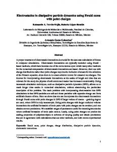
Figure 2.1: Illustration of the different integration contours in Cartesian (TOP) and spherical (BOTTOM) coordinates. The Irving-Kirkwood contour (LEFT) is the same in both cases, while the Harasima contour (RIGHT) depends on the coordinates.
ambiguity arises from the expression for p C ij,αβ , which can be obtained by comparison with the continuum mechanics expression for the momentum density [Ikeshoji, 2005] Z C pij,αβ (r) = − fij,α δ(r − l) rˆβ dl. (2.142) Cij
The integration contour Cij is in principle arbitrary, and in general f ij depends on Cij . The arbitrariness of Cij and the resulting ambiguity in the local pressure tensor has been discussed several times in the literature [Irving and Kirkwood, 1950; Harasima, 1952; Schofield and Henderson, 1982]. There are basically two choices for the contour C ij : the Irving-Kirkwood (IK) definition and the Harasima (H) definition. The IK definition is just the straight line joining the two particles i and j. The H definition of the contour C ij depends on the coordinates (spherical or cartesian) of the local sub-volume and goes parallel to its boundaries. Both contour definitions are illustrated in figure 2.1. For quantities that do not depend on the local pressure profile, both choices yield the same results. The expressions for the local pressure tensor, however, differ between the two methods. It was shown by Ikeshoji et al. [2003] that the H-contour does not give a uniform pressure in uniform liquids, and other authors also argue that the IK scheme should be favored [Varnik et al., 2000; Hafskjold and Ikeshoji, 2002; Heinz et al., 2004]. We can perform the integral in equation (2.142) with the IK-contour and finally get an expression for the pressure tensor + * * + X ∆rij 1 X 1 fij,α rij,β , (2.143) Pαβ (Vl ) = mi vi,α vi,β + Vl Vl rij i∈Vl
rij ∩Vl 6=∅
where the sum runs over all pairs of particles whose connecting line has a non-vanishing fraction ∆rij /rij that lies within the volume Vl . Note that there will also be contributions from pairs where neither of the particles lies within the volume. The length of r ij that lies in Vl is denoted by ∆rij .
30
2.6 Coarse-Graining The choice of the IK contour has removed the ambiguity and led to a definite expression for the local pressure tensor. We will adopt the Irving-Kirkwood scheme later in this work to devise an algorithm for computing the local pressure tensor in a molecular dynamics simulation.
2.6 Coarse-Graining We have already seen that it is not always appropriate to deal with all degrees of freedom explicitly. In many cases, a description on a larger length scale is completely sufficient. The transition from a description with many degrees of freedom on a small scale to a description on a larger scale with reduced degrees of freedom is called coarse-graining. 9 The limits of this process are on the one hand the microscopic description of classical mechanics, and on the other hand the macroscopic description of thermodynamics. All levels in between are termed mesoscopic. Mesoscopic scales are often important in complex fluids, where alongside the continuum behavior of some solvent, structure is present on an intermediate length scale. Examples include liquid crystals, colloidal suspensions, turbulent flows or biological systems like vesicles, micelles or membranes. Coarse-graining is an important technique if one deals with computer simulations. Despite the power of modern computers, computational resources are still limited. Coarse-grained simulation techniques provide a twofold enhancement: Firstly, computational costs are reduced because fewer degrees of freedom have to be simulated. Secondly, since the degrees of freedom represent larger time scales, a much larger time span can be simulated. A coarse-grained model is usually constructed by hand, based on more or less sound physical reasoning. Issues involved are for example conserved quantities, symmetries and invariances, and of course simplicity. The justification of a specific model is given by comparing predictions with experimental results. It is thus a rather phenomenological approach. To put it on a more rigorous basis, one has to establish the link to the microscopic theory. In the following, I will describe the microscopic foundations of coarse-graining. The presentation is along the lines of Espa˜nol [2003].
2.6.1 Levels of Description Before we go into the mathematical details, we briefly review some important levels of description. To characterize a level of description one has to specify the relevant variables whose evolution is of interest. The different levels of description form a hierarchy, in which the order is determined by the amount of information that is represented by the set of relevant variables. Table 2.1 on page 33 summarizes several common levels of description for the example of a colloidal suspension [the example is originally due to Espa˜nol, 2003]. More detailed levels have more relevant variables while coarser levels have a reduced number of variables and hence capture less information. Included in the hierarchy is also the time scale on which phenomena can be described. Due to the elimination of fast degrees of freedom in a coarse-grained level, only phenomena on larger time scales can be described correctly. The evolution of the relevant variables is described by an equation of motion. 9
This is similar in spirit to Espa˜nol [2003], who defines: “The process of representing a system with fewer degrees of freedom than those actually present in the system is called coarse-graining.”.
31
2 Theoretical Foundations The limiting cases of the hierarchy of coarse graining are the microscopic description of classical mechanics on one side and the macroscopic description of thermodynamics on the other. In classical mechanics, every degree of freedom present in the system is included in the description and the equations of motion are the Hamiltonian equations (or any equivalent formulation). In thermodynamics, the relevant variables are the dynamical invariants of the system. At this level, there is no equation of motion because the relevant variables characterize a steady state of the system. The aim of a microscopic foundation of coarse-graining is to derive the equation of motion for the coarse-grained variables from the degrees of freedom on a more detailed level. This must not necessarily be the microscopic level, but it can be every mesoscopic level as long as its relevant variables capture more information. An important issue in coarse-graining is the separation of the time scales. On a coarse-grained level, only phenomena on larger time scales can be described correctly. The time scales of the eliminated degrees of freedom are not captured explicitly, but they may be inherent in the equations of motion for the coarse-grained variables. If a clear separation of time scales exists, the evolution equations for the relevant variables are Markovian, i.e. there is no memory for past states of the relevant variables. This case is mathematically much more convenient to treat because the integrodifferential equations for non-Markovian processes are replaced by usual differential equations for Markovian processes. The process of eliminating degrees of freedom involves a loss of information. As a consequence thereof, the future state of the coarse-grained variables cannot be predicted with certainty, as many microscopic configurations may be compatible with the present coarse state. Therefore, the coarse-grained variables must have a probabilistic description and the evolution equations contain stochastic terms. The appropriate description of the coarse-grained system is thus in terms of a probability distribution for the relevant variables, and the evolution equation contains dissipative and fluctuating terms. In the Markovian case the evolution equation is a Fokker-Planck equation. The derivation of this Fokker-Planck equation is the main goal of the theory of coarse-graining. The mathematical formalism for this purpose was developed by Zwanzig [1961] using the projection operator technique [cf. Espa˜nol, 2003, and the references therein]. It can be used to derive the coefficients for the Fokker-Planck equation from the microscopic degrees of freedom or from any mesoscopic degrees of freedom containing more detail. The basics of the theory of coarse-graining are sketched in the next sections.
2.6.2 Theory of Coarse Graining Microscopic Level We will consider only the basic case of obtaining the Fokker-Planck equation at a mesoscopic level from the microscopic description of classical mechanics. The equation of motion at this level is Hamilton’s equation, which can be written in compact form � � 0 1 ˙Γ = L0 ∂H , . (2.144) L0 = −1 0 ∂Γ In classical mechanics, the evolution equation for the probability density of the degrees of freedom is the Liouville equation (2.15). Under the assumption of mixing dynamics the system will reach
32
2.6 Coarse-Graining level of description Classical Mechanics Hydrodynamics Fokker-Planck Smoluchowski Fick diffusion Thermodynamics
relevant variables {ri , pi , Ri , Pi } ρ(r), p(r), �(r) {Ri , Pi } {Ri } c(r) E, M, P, . . .
equation of motion Hamilton’s equations Navier-Stokes equations Fokker-Planck equation Smoluchowski equation Fick’s diffusion law none
Table 2.1: Different levels of description for a colloidal suspension. For each level the set of relevant variables and the respective equation of motion are listed. The example is taken from [Espa˜nol, 2003].
a stationary state where ∂t ρ(Γ; t) = 0.
(2.145)
The stationary state is a function of the dynamical invariants of the system, where a dynamical invariant is defined through d I(Γ) = 0, (2.146) dt that is, it does not change in time. Examples for dynamical invariants are the energy H(Γ) and the total momentum P(Γ). The stationary state can be written lim ρ(Γ; t) = ρ0 (Γ) = ρ˜0 (I(Γ)),
t→∞
(2.147)
where ρ0 (Γ) denotes the equilibrium ensemble of the system. Let P (I(Γ)) be the probability distribution of the dynamical invariants and P 0 (I(Γ)) its equilibrium pendant. The equilibrium ensemble is completely determined by the probability distribution P 0 (I) of the dynamical invariants in equilibrium P0 (I(Γ)) , (2.148) ρ0 (Γ) = Ω0 (I(Γ)) where Ω0 (I) is the measure of the hypersurface in phase-space on which the dynamical invariants have the prescribed values I Z Ω0 (I) =
dΓ δ (I(Γ) − I) .
(2.149)
Since it follows from the Liouville equation that P (I(Γ)) is itself invariant, the equilibrium ensemble is completely determined by the initial distribution of the dynamical invariants. So from the precise knowledge of the dynamical invariants I 0 at time t = 0 we get the equilibrium distribution δ (I(Γ) − I0 ) ρ0 (Γ) = = ρmic (Γ), (2.150) Ω0 (I0 ) which resembles the microcanonical ensemble. Coarse-grained Level We now switch to a mesoscopic level, for which the state of the system is described by certain dynamical variables X(Γ). These coarse-grained variables evolve in time as the microscopic state Γ evolves. The time derivative of the variables X(Γ) is in the Liouville formulation d X(Γ(t)) = iLX(Γ(t)), dt
(2.151)
33
2 Theoretical Foundations which has the formal solution X(Γ(t)) = exp(iLt)X(Γ(0)).
(2.152)
As pointed out in the last section, the evolution of the coarse-grained variables contains stochastic terms because many microscopic states may be compatible with the coarse state. Consider for example two microscopical configurations Γ 1 and Γ2 with X(Γ1 ) = X(Γ2 ). After some time, the corresponding coarse states may have evolved to different values X(exp(iLt)Γ 1 ) 6= X(exp(iLt)Γ2 ). Therefore, we have to describe the coarse-grained variables by a distribution function Z P (x; t) = dΓ δ (X(Γ) − x) ρ(Γ; t). (2.153)
The stochasticity in the actual values of X comes basically from missing knowledge about the initial microscopic state described by ρ(Γ; 0). Usually we have only P (x; 0), hence ρ(Γ; 0) has to be determined such that it is compatible with equation (2.153) at time t = 0. However, this does not define ρ(Γ; 0) unambiguously because many distributions can produce the desired P (x; 0). According to the principle of maximal ignorance, we choose the distribution ρ that maximizes the entropy Z ρ(Γ) . (2.154) S[ρ] = −kB dΓ ρ(Γ) ln ρ0 (Γ) The solution can be obtained by the method of Lagrange multipliers. We get ρ(Γ) =
P (X(Γ); 0) , Ω(X(Γ))
where Ω(x) is the measure of the hypersurface in phase-space that is compatible with x Z Ω(x) = dΓ δ (X(Γ) − x) ρ0 (Γ).
(2.155)
(2.156)
This resembles equation (2.153), and hence Ω(x) is the equilibrium distribution function for the coarse-grained variables. The time evolution of P (x; t) in equation (2.153) is determined by the time evolution of ρ(Γ; t). On the coarse-grained level, we want to have an equation of motion for P (x; t) that is independent of the microscopic evolution of ρ(Γ; t). This problem of finding a closed form for P (x; t) is similar to obtaining a closed form for a distribution function in the BBGKY hierarchy (cf. section 2.3.2). The solution here is Zwanzig’s projection operator technique. The projection operator P is defined by PF (Γ) = hF iX(Γ) ,
(2.157)
where the constrained average is given by 1 hF i = Ω(x) x
Z
dΓ ρ0 (Γ)Ψx (Γ)F (Γ).
(2.158)
For convenience we have introduced Ψx (Γ) = δ (X(Γ) − x) .
34
(2.159)
2.6 Coarse-Graining hF ix is the expectation value of the function F in the subspace where the relevant variables have the prescribed values x. The application of the projection operator P to a function of phase spaces yields a function of the relevant variables X(Γ). P satisfies the usual properties of a projection operator. The complementary operator is Q = 1 − P. The operators P and Q are used to introduce the operator identity Z t dt0 exp(iLt0 )PiLQ exp(iLQ(t − t0 )) + Q exp(iLQt). (2.160) exp(iLt) = exp(iLt)P + 0
With the help of this identity and the chain rule iLΨx (Γ) = iLXi
∂ Ψx (Γ) ∂xi
(2.161)
we can derive the time evolution of Ψ x (Γ), which then leads to the time evolution of P (x; t) in a closed form ∂ vi (x)P (x; t) ∂xi Z Z t ∂ ∂ P (x0 ; t0 ) 0 dt dx0 Ω(x0 ) Dij (x, x0 , t − t0 ) 0 . + ∂xi ∂xj Ω(x0 ) 0
∂t P (x; t) = −
(2.162)
In this equation, the drift vi (x) and the diffusion Dij (x, x0 , t) have been introduced. The expressions for them are vi (x) = hiLXi ix , D E x0 0 Dij (x, x0 , t) = (iLXj − hiLXj ix ) exp(iLQt)Ψx (iLXi − hiLXi ix ) .
Note that
Z
dΓ ρ(Γ; 0)Q exp(iLQt)QiLΨx (exp(iLt)Γ) = 0
(2.163) (2.164)
(2.165)
because the initial ensemble ρ(Γ, 0) is a function of the relevant variables X(Γ) only. The integro-differential equation (2.162) is exactly equivalent to the Liouville equation. It is difficult to solve, but in the current form it can be simplified by applying the Markovian assumption. That is, if a clear separation of the time scales of the microscopic and coarse-grained degrees of freedom exists, we can assume that the probability distribution P (x; t) is approximately constant in the time the diffusion tensor Dij (x, x0 , t − t0 ) needs to decay. We can then write Z t Z ∞ 0 0 0 dt D(t − t )P (t ) ≈ P (t) dt0 D(t0 ). (2.166) 0
0
This approximation is correct up to terms of second order in iLX, and we can write exp(iLQt)Ψx QiLX = Ψx exp(iLQt)QiLX + . . .
(2.167)
It is now possible to rewrite the diffusion tensor D ij (x, x0 , t) such that it becomes diagonal in x, x0 . We define Z ∞
�x dt0 (iLXj − hiLXj ix ) exp(iLQt0 )(iLXi − hiLXi ix ) (2.168) Dij (x) = 0
35
2 Theoretical Foundations and finally arrive at the equation ∂t P (x; t) = −
∂ ∂ ∂ P (x; t) vi (x)P (x; t) + Ω(x)Dij (x) . ∂xi ∂xi ∂xj Ω(x)
(2.169)
This is the Fokker-Planck equation for the probability distribution of the coarse-grained variables, which describes the time evolution of the system on the coarse-grained level. The microscopic degrees of freedom do not appear explicitly, but they are implicit in the drift v i (x) and diffusion Dij (x). It should be emphasized that only phenomena on time scales larger than the decay of the correlation in Dij (x) are described correctly. Shorter time scales are not in the scope of this description. Moreover, the coarse-grained Fokker-Planck equation is only valid if there is a clear separation of time scales (i.e. the Markovian assumption is justified). The validity of this assumption is difficult to verify in practice and can often only be tested afterwards by comparison with experimental results.10 The construction of coarse-grained descriptions thus requires a good amount of physical intuition regarding the choice of the relevant variables.
2.6.3 The GENERIC Structure The theoretical framework described in the last section is useful in deriving the Fokker-Planck equation for coarse-grained levels of description from the underlying microscopic dynamics. For a computer simulation, however, one would be more interested in an evolution equation for the relevant variables themselves. Mathematically, this boils down to writing the stochastic differential equations that are equivalent to the Fokker-Planck equation. In this section, I will describe how this can be done for the GENERIC structure. GENERIC stands for ‘General Equation for Non-Equilibrium Reversible Irreversible Coupling’. The GENERIC structure was first introduced ¨ ¨ by Grmela and Ottinger [1997]; Ottinger and Grmela [1997] in a heuristic manner. The same au¨ thors put it onto theoretical grounds by application of the projection operator technique [ Ottinger, 1998]. A system has the GENERIC structure, if the dynamical invariants on the microscopic level can be written as functions of the coarse-grained variables, i.e. ˜ I(Γ) = I(X(Γ)).
(2.170)
This is a rather strong property, but the GENERIC structure that emerges from it is in turn quite powerful. As a special case, the Hamiltonian can be written as ˜ H(Γ) = H(X(Γ)) ≡ E(X(Γ)).
(2.171)
If (2.170) holds, then the equilibrium ensemble ρ 0 (Γ) is a function of the dynamical invariants only and the equilibrium distribution of the relevant variables becomes Z ˜ Ω(x), (2.172) Ω(x) = dΓ ρ0 (Γ)Ψx (Γ) = ρ˜0 (I(x)) where Ω(x) measures the volume in phase-space where the relevant variables take the prescribed values Z Ω(x) = dΓ Ψx (Γ). (2.173) 10
For liquids, the Markovian assumption is actually not valid because memory effects can not be neglected. This is the starting point for mode coupling theory.
36
2.6 Coarse-Graining The constrained average takes the form Z 1 ˜ dΓ ρ˜0 (I(x))Ψ hF i = x (Γ)F (Γ) ˜ ρ˜0 (I(x)) Ω(x) Z 1 = dΓ Ψx (Γ)F (Γ). Ω(x) x
(2.174)
We can rewrite the time evolution of a relevant variable as ∂Xi ˙ ∂Xi Γ iLΓ = ∂Γ ∂Γ ∂Xi ∂H(Γ) = L0 ∂Γ ∂Γ ∂Xi ∂Xj ∂E(X(Γ)) = L0 , ∂Γ ∂Γ ∂xj
iLX =
(2.175)
where E(x) is the Hamiltonian expressed in terms of the relevant variables. The drift v i (x) then becomes ∂E(x) , (2.176) vi (x) = hiLXi ix = Lij (x) ∂xj where the operator L(x) is introduced as the coarse pendant of L 0 � � ∂Xi ∂Xj x L0 . Lij (x) = ∂Γ ∂Γ
(2.177)
Because of the similarity of the right hand side of (2.176) with the Hamiltonian equation (2.144), the operator L(x) is called reversible operator, and L(x) ∂E(x) ∂x is the reversible dynamics of the relevant variables X. We further introduce D(x) , kB S(x) = kB ln Ω(x),
M (x) =
(2.178) (2.179)
where S(x) is an entropy-like expression (Ω(x) counts the microstates compatible with the coarse state). We arrive at the GENERIC form of the Fokker-Planck equation � � ∂S ∂ ∂E + M (x) ∂t P (x; t) = − L(x) P (x; t) ∂x ∂x ∂x (2.180) ∂ ∂ S + kB M (x) P (x; t), ∂x ∂x where M S (x) is the symmetric part of the diffusion tensor. The stochastic differential equation equivalent to this Fokker-Planck equation is � � ∂S ∂E S + M (x) + kB ∇M (x) dt + d˜ x, (2.181) dx = L(x) ∂x ∂x where we have adopted the Itˆo interpretation. The d˜ x are linear combinations of Wiener increments and they satisfy the fluctuation-dissipation relation d˜ x(t)d˜ x T (t) = 2kB M S (x(t))dt.
(2.182)
37
2 Theoretical Foundations At this point, it is worth noting that the definition of the diffusion tensor D ij has the form of a Green-Kubo relation. It is possible to identify the term exp(iLQt)(iLX i − hiLXi ix ) with Gaussian white noise ζ(t).11 The fluctuation dissipation relation is then written in the common form hζ(t)ζ(t0 )i = 2kB M (x)δ(t − t0 ). (2.183) If we assume that the building blocks of E, S, L, M do not depend on k B , then in the limit kB → 0 the stochastic differential equation (2.181) becomes x˙ = L(x)
∂S ∂E + M (x) . ∂x ∂x
(2.184)
Here, the fluctuating term has vanished, and the dynamics is purely deterministic. L(x) ∂E ∂x is is the irreversible part. Further, we have the the reversible part of the dynamics, and M (x) ∂S ∂x GENERIC degeneracies ∂S = 0, ∂x ∂E = 0. M (x) ∂x L(x)
(2.185) (2.186)
This leads to ∂E ˙ x˙ = 0, E(x) = ∂x ∂S S ∂S ∂S ˙ x˙ = M (x) ≥ 0, S(x) = ∂x ∂x ∂x
(2.187) (2.188)
which turn out to be the first and second law of thermodynamics, basically. Thus, the GENERIC structure is consistent with thermodynamics. The terms reversible and irreversible part of the dynamics and the degeneracy properties have led to the the name General Equation for NonEquilibrium Reversible Irreversible Coupling (GENERIC). The GENERIC structure can be used to derive coarse-grained models for the simulation of complex systems. As an important advantage over ad-hoc constructions, the GENERIC structure will lead to models that include the essential stochastic parts of the coarse-grained dynamics in a thermodynamically consistent way. While we have here only considered the link between the microscopic and a mesoscopic level of descrip¨ tion, it is also possible to relate different mesoscopic levels of description [ Ottinger, 1998]. The key feature of the GENERIC structure is the separation of the dynamics into the reversible and irreversible parts. Many non-equilibrium systems can be expressed in these terms, like hydrodynamics, polymer dynamics or chemical reaction dynamics. It is therefore reasonable, despite the ˜ strong assumption I(Γ) = I(x), to use the framework to derive new coarse-grained models. An instructive example in the context of dissipative particle dynamics is the soft fluid particle model which will be discussed in section 3.8.
11
In a mathematical sense, this is not strict because ζ(t) would be the time derivative of d˜ x, which actually is not differentiable [Gardiner, 1994]. However, the introduction of Gaussian white noise is a common rule of thumb.
38
3 Dissipative Particle Dynamics Among the complex systems studied with computer simulations are soft matter systems that often consist of a liquid environment in which the objects of interest are dissolved. These objects may be colloids or polymers in solution, or even biological building blocks like micelles or membranes. Since the behavior of such systems can be much more complex than that of a simple fluid, they are also called complex fluids. The dynamics of a complex fluid is fundamentally affected by its microscopic structure. As a consequence, a complex fluid is no longer completely described by the Navier-Stokes equation. This is due to the disparate length scales which influence the dynamics, that is, the observed phenomena on the macroscopic scale are caused by the constituents that exist on the microscopic scale. The presence of these disparate length scales poses a problem for computer simulations. Numerical solvers for the Navier-Stokes equation are inadequate because the microscopic structure of the complex fluid cannot be incorporated properly. Molecular Dynamics (MD) simulations on the microscopic level are also inappropriate, as overly long simulation runs are necessary to study macroscopic phenomena. Equilibrium situations can to some extend be investigated with Monte Carlo simulations, but it is not straightforward how to interpret dynamical issues in this method. Therefore, new techniques are needed to bridge the gap between the microscopic and the macroscopic level. Mesoscopic simulation methods try to overcome the problems by using the information about the characteristic length scales of the system to devise new models for complex fluids and efficient computational techniques. They aim at modeling the fluid on some intermediate or mesoscopic length scale that captures the relevant dynamics. The formal foundation for mesoscopic simulation techniques is the theory of coarse-graining described in section 2.6. However, many mesoscopic simulation methods are not strictly derived in a mathematical sense, but they are constructed in a way that satisfies certain conservation laws or symmetries that are considered to be essential for the observable phenomena. One of the first mesoscopic approaches were the lattice gas automata (LGA) introduced by Frisch et al. in 1986 [see Raabe, 2004, for a review]. In this method, the constituent particles of the fluid move simultaneously from site to site on a regular lattice. This is schematically depicted in figure 3.1. The evolution of the system is described by a set of collision rules for the particles. The computational costs per particle are reduced considerably compared to molecular dynamics. The lattice gas approach yields correct hydrodynamics, and the time step in lattice gas simulations can be much larger than in molecular dynamics simulations. The change in the particle positions during one LGA time step is typically on the order of the mean free path. In the alternative lattice Boltzmann approach, the lattice nodes are described by distribution functions. The evolution of the system is splitted into a propagation phase, in which the particle distribution is changed according to the current motion, and a collision phase, in which the velocities are adopted according to certain collision rules. Lattice Boltzmann (LB) is originally an extension of the lattice gas, but the lattice Boltzmann equation (LBE) can also directly be derived from the continuous Boltzmann equation.
39
3 Dissipative Particle Dynamics In this sense, a lattice Boltzmann simulation provides a numerical solution of the Boltzmann equation. The introduction of a lattice in the LGA and LB approaches causes two fundamental problems: Galilean invariance and isotropy are both broken on the lattice. Although in some cases this can be cured by choosing other lattice geometries (i.e. lattices with sufficient rotational symmetry like the hexagonal lattice) or by rescaling the velocities, this remains in general a severe drawback of the method. Furthermore, the incorporation of boundary conditions in LGA and LB simulations is not an easy task, hence the extension to more complicated systems can be rather cumbersome. The computational costs increase accordingly, and the simplicity of the model is more than counterbalanced [Hoogerbrugge and Koelman, 1992]. Another technique to cope with different scales in a system is the Langevin method introduced in section 2.4.3. In this approach, the fast degrees of freedom are eliminated completely and replaced by friction and random forces. This is especially appealing for fluid systems where the structure of the solvent is uninteresting. The explicit simulation of the solvent particles in a molecular dynamics simulation is very expensive because usually the number of solvent particles is large. On the other hand, no interesting information is obtained by dealing with the solvent explicitly. Therefore, an inexpensive method to treat the solvent is in general highly desirable, and much effort is devoted to develop efficient solvent models for computer simulations [Farago, 2003; Lenz and Schmid, 2005]. An approximate approach like Langevin dynamics is very tempting, but unfortunately the Langevin method is rather useless for complex fluids because it does not produce correct hydrodynamics. The reason for this is that the random and friction forces do not conserve momentum, which is a basic requirement for hydrodynamic behavior. As a consequence, Langevin dynamics produces behavior that is diffusive but not hydrodynamic. This chapter is devoted to the introduction of dissipative particle dynamics (DPD). Dissipative particle dynamics is a particle based mesoscopic simulation method for isothermal complex fluids. It does not suffer from the drawbacks of previous methods, i.e. it satisfies Galilean invariance and isotropy, and it conserves mass and momentum. Basically, dissipative particle dynamics combines the advantages of the methods while avoiding their subtleties. This is done by introducing the LGA-like time stepping into molecular dynamics combined with Langevin-type dissipative and stochastic forces. The idea is to use continuous variables for the positions and velocities of the particles and update them in a propagation and a collision step. The collisions are determined by pairwise additive forces between the particles which are considered to be soft and finite. In this way, one gets rid of the lattice while retaining the possibility to use a large time step. The updating of the positions and momenta of the particles can be done in a standard MD fashion. In order to achieve a coarse-grained level of description, the interparticle forces contain dissipative and stochastic contributions. The important point is that the forces are constructed such that mass and momentum are conserved. Dissipative particle dynamics is – as the name suggests – a particle based method. A dissipative particle (DP), however, is not identified with a physical particle of the fluid, but represents the center of mass of a mesoscopic portion of fluid. The idea of the dissipative particle dynamics method in comparison to the lattice gas approach is illustrated in figure 3.1. Dissipative particle dynamics has a number of advantages: Firstly, the lack of a lattice yields Galilean invariance and isotropy, and in practice it is much less cumbersome to include boundaries than in the lattice approaches. Secondly, since DPD conserves mass and momentum by construction, it is expected to produce correct hydrodynamic behavior. Thirdly, being a particle based method, DPD is quite versatile with respect to addition of new model features. Complex
40
3.1 A Short History of Dissipative Particle Dynamics
rc v
Figure 3.1: Illustration of the lattice gas approach (LEFT) in comparison to the dissipative particle dynamics method (RIGHT). In the lattice gas, particles move on a lattice and change their velocities according to certain collision rules. In dissipative particle dynamics, the particles have continuous positions and interact through pairwise forces that contain a conservative, a dissipative and a random part.
fluid structures can be modeled straightforwardly by introducing different particle types with corresponding interactions. Further extension are possible by introducing internal variables for the dissipative particles, e.g. internal energies or charges. Therefore, DPD seems a very promising technique for the simulation of complex fluids and soft matter systems. The remainder of this chapter is organized as follows: I start with the history of dissipative particle dynamics before I introduce the method itself in section 3.2. From the stochastic differential equations describing the evolution of the DPD system, the equivalent Fokker-Planck equation can be deduced, which will be done in section 3.3. Then a H-theorem can be derived in section 3.4 that ensures the approach of a well-defined equilibrium distribution. In section 3.5, we derive the hydrodynamic equations for DPD. The role of the finite time step will be discussed in section 3.6. The original DPD model is isothermal, but it is possible to extend the method to obtain an energy conserving system. This extension will be presented in section 3.7. I sketch in section 3.8 the microscopic foundations of the DPD model. In particular, I will outline the Voronoi fluid particle model and the soft fluid particle model. Finally, I present two theories for the transport properties of the DPD model, namely the theory of Marsh, Backx and Ernst and the Boltzmann theory for DPD. These theories will be used in chapter 5 to compare the simulation results.
3.1 A Short History of Dissipative Particle Dynamics Dissipative particle dynamics was originally proposed by Hoogerbrugge and Koelman in 1992 as a new method for simulating hydrodynamic phenomena. It combines the best of both molecular dynamics and lattice gas approaches. It obeys Galilean invariance and isotropy and conserves mass and momentum by construction. In the original contribution, it was verified both analytically and by simulations that correct hydrodynamic behavior is produced. The coarse-grained variables satisfy the Navier-Stokes equation to lowest order in the field gradients. In a simulation, it was shown that low Reynolds number flow through an array of infinite cylinders approaches the Stokes flow limit with increasing system size. This is in accordance with generalized hydrodynamics.
41
3 Dissipative Particle Dynamics Subsequently, dissipative particle dynamics was used for simulations of hard-sphere suspensions under steady shear [Koelman and Hoogerbrugge, 1993] and polymer solutions [Madden et al., 1994; Schlijper et al., 1995]. The dissipative and stochastic forces in DPD are Langevin-like and do not conserve the energy of the system. There is no transport of energy and the model is expected to be isothermal. However, in the original algorithm there is no expression relating the model parameters to the temperature of the system. This was established by Espa˜nol and Warren [1995], who derived the correct fluctuation dissipation relation for the friction and noise terms in dissipative particle dynamics. Deriving the Fokker-Planck equation corresponding to the DPD equations of motion, they obtained the condition under which the steady-state solution is the Gibbs canonical ensemble with a well defined temperature. They also observed in simulations that discretization errors due to finite time steps lead to deviations from the prescribed equilibrium temperature. Further investigations have clarified several aspects of DPD and led to rigorous theoretical justifications of the method. Espa˜nol [1995] has derived the hydrodynamic equations for the mass and momentum density fields by applying the projection operator technique. Thereby, the connection of the speed of sound and the viscosity coefficients of the fluid to the model parameters, i.e. the friction coefficient and the noise amplitude, was clarified. It was further discussed for which temperature range a Newtonian description of the fluid is valid and when non-Newtonian responses would arise. Groot and Warren [1997] review dissipative particle dynamics and discuss how the friction coefficient, noise amplitude and time step may be chosen. They discussed the useful parameter ranges of soft conservative potentials and mapped the model parameters onto Flory-Huggins theory for polymers. They observed that the dynamics of the polymer and the fluid may couple, i.e. the time scales for particle transport and momentum diffusion overlap. Marsh [1998] analyzed several theoretical aspects of dissipative particle dynamics. An analytic expression for the dependence of the equilibrium temperature on finite time steps was obtained by Marsh and Yeomans [1997]. This was achieved by following the evolution of the one-particle distribution function under the finite time step algorithm. A stability bound for given model parameters was found. The Fokker-Planck-Boltzmann equation for dissipative particle dynamics was derived by Marsh et al. [1997a] and was shown to obey an H-theorem that guarantees existence and approach of a unique equilibrium. From the Fokker-Planck-Boltzmann equation the macroscopic evolution equations were obtained using the Chapman-Enskog method [Marsh et al., 1997b]. Thereby, explicit expressions for the thermodynamic and transport properties were obtained. Analytic results for the static and dynamic properties were compared with numerical simulations showing sizable differences between simulated and predicted results. These could partially be explained by Masters and Warren [1999], who applied the Boltzmann pair collision theory to dissipative particle dynamics. They found that the previous theory corresponds to a weak scattering limit (Vlasov limit) and observed a new scaling behavior of the transport coefficients for strong dissipation. Detailed balance and H-theorems can be extended to multicomponent fluids [Coveney and Espa˜nol, 1997; Marsh and Coveney, 1998]. Marsh [1998] also made an approach towards generalized hydrodynamics for dissipative particle dynamics, which must be used if the length scales of the system can not be separated clearly. The dynamical regimes of dissipative particle dynamics were investigated further by Serrano et al. [1999]; Espa˜nol and Serrano [1999]. By looking at the velocity autocorrelation function these authors identified two dynamical regimes: The low friction regime can be described in terms of a mean field theory, and the kinetic theory gives good predictions [see Ripoll Hernando, 2002]. For high friction, the behavior is hydrodynamic and collective effects become important.
42
3.1 A Short History of Dissipative Particle Dynamics Several extensions have been proposed for dissipative particle dynamics. As dissipative particle dynamics is an isothermal model, no energy transport and heat flux can be simulated. To overcome this limitation an energy conserving extension of DPD was developed independently by Bonet Avalos and Mackie [1997] and Espa˜nol [1997b]. The dissipative particles get an additional variable for the internal energy, and the corresponding evolution equation is derived consistently. The internal energy is coupled to the dissipative forces between the particles, and a fluctuation dissipation relation ensures the correct equilibrium distribution. The energy conserving variant of DPD was used to simulate heat conduction [Ripoll et al., 1998], and the dynamical and transport properties were analyzed [Bonet Avalos and Mackie, 1999]. Other extensions aim at modeling viscoelastic flow or chemical reactions. The additional internal variables can be coupled to the conventional hydrodynamic variables in a thermodynamically consistent way by using the GENERIC framework [see Espa˜nol, 2002, and references therein]. Another interesting extension is the combination of dissipative particle dynamics with Monte Carlo techniques [Willemsen et al., 1998]. In this way, efficient sampling schemes can be applied, like the Gibbs ensemble technique or configurational bias Monte Carlo. The technique can be used to simulate phase equilibria and for free energy calculations. The combination of DPD and Monte Carlo is in general a versatile technique to simulate ensembles other than the N V T -ensemble. For example, a DPD-MC approach has been applied to constant-tension simulations of lipid bilayers [Venturoli and Smit, 1999; Kranenburg, 2004, and the references therein]. The sizable discretization errors that lead to a dependence of the equilibrium properties on the time step have directed interest to the development of improved numerical algorithms. Instead of the conventional Euler scheme, Groot and Warren [1997] used a modified version of the VelocityVerlet algorithm, in which a tunable parameter λ is used to make a prediction of the new velocities. The original Velocity-Verlet algorithm is recovered for λ = 1/2, and actually both algorithms produce identical trajectories [den Otter and Clarke, 2000]. Another approach was put forward by Pagonabarraga et al. [1998], who introduced a self-consistent algorithm. The updating of the velocities is performed such that the final values of the forces and velocities are consistent. This is necessary because the forces acting on a particle depend on the velocities of neighboring particles. The self-consistent algorithm is not plagued by the strong ∆t-dependence of previous algorithms. Gibson et al. [1999] proposed an intermediate approach, which is basically an extension of the modified Velocity-Verlet algorithm with an additional second update of the dissipative forces at the end of the integration step. Novik and Coveney [1998] discuss finite-difference methods and their application to models with non-conservative forces. With particular reference to dissipative particle dynamics, they recommend the algorithm of Gibson et al. [1999] as a superior one. A completely different approach was formulated by Lowe [1999]. While retaining the key features of momentum and temperature conservation, it does not use dissipative and random forces at all. Instead, the system is integrated with conservative forces only and then thermalized to the prescribed temperature with an Anderson thermostat. This frees the algorithm from the requirement of a self-consistent solution and makes it possible to control the dynamical parameters of the system much easier. Another way to cope with the velocity dependence of the dissipative forces was taken by den Otter and Clarke [2001]. They exploit the analogy between DPD and stochastic dynamics to derive a modified leap-frog algorithm, in which the relative strength of the dissipative and random forces is described by parameters α, β. These parameters are determined in advance by simulating a system for which the equilibrium properties are known to be consistent. Finally, there are techniques that use the Trotter expansion to factorize the integration step. For the multivariate Langevin equation and the Kramers equation, fourth-order algorithms were developed by
43
3 Dissipative Particle Dynamics Forbert and Chin [2000]. For dissipative particle dynamics, integrators based on first and second order splitting were suggested [Shardlow, 2003]. Very recently, stochastic Trotter schemes were used to devise mathematically correct and efficient numerical integrators for different stochastic models [de Fabritiis et al., 2005]. Several of the described integration schemes for dissipative particle dynamics have been extensively tested and compared with respect to their performance [Besold et al., 2000; Vattulainen et al., 2002; Nikunen et al., 2003]. This has also shed some light on the integrator-induced effects in simulations of complex systems. The versatility of dissipative particle dynamics and its theoretically justified properties make it an appealing method for coarse-grained simulations of complex systems. However, as DPD is an ad-hoc construction, it is not a-priori clear how the concept of a dissipative particle can be related to the microscopic degrees of freedom. This deficiency has been solved through a derivation of DPD-type equations from microscopic dynamics via systematic coarse-graining (cf. section 3.8). There are basically two approaches of coarse-graining for DPD, namely Voronoi fluid particles and a variant of smoothed particle hydrodynamics. Voronoi fluid particles were introduced by Flekkøy and Coveney [1999] to define the dissipative particles as cells on a Voronoi lattice with variable sizes. The equations of motion for these particles can be derived from the microscopic dynamics and lead to equations very similar to conventional DPD [Flekkøy et al., 2000; de Fabritiis et al., 2002]. The derivation is based on the Fokker-Planck formalism for the equilibrium distribution of the set of variables. An alternative derivation is based on the GENERIC framework (cf. section 2.6.3) and thus guarantees thermodynamical consistency. The latter method is reported to yield higher numerical accuracy [Serrano et al., 2002]. The Voronoi fluid particle model can be used in multi-scale modeling of complex fluids, i.e. the size of the Voronoi particles is locally adjusted to the length scales that are present in the system [de Fabritiis et al., 2002; de Fabritiis and Coveney, 2003]. Smoothed particle hydrodynamics is a method originally developed in astrophysical contexts. The similarity to DPD was pointed out by Espa˜nol et al. [1997]; Espa˜nol [1998], and the formalism was worked out by Espa˜nol [2002]; Espa˜nol and Revenga [2003]. The smoothed particles are spherical particles defined by a bell-shaped weight function (e.g. the Lucy function), and the equations of motion are derived using the GENERIC framework. Both fluid particle models link the coarse-grained equations of motion to the microscopic dynamics. This establishes a microscopic foundation of those fluid particle models, and since the DPD-equations are very similar, this also provides a sound justification for dissipative particle dynamics. One of the original ideas of dissipative particle dynamics is to use soft potentials for the conservative interactions in order to be able to use a large time step. However, this is not strictly necessary, and actually it turned out that a large time step may be responsible for sizable discretization errors in the measured variables. As a matter of fact, there are two different aspects of DPD: soft conservative interactions on the one hand and thermostatting on the other. The latter is achieved by the dissipative and random forces. As pointed out by Soddemann et al. [2003], the two aspects are completely independent. It is no problem to use DPD with conventional interactions such as Lennard-Jones potentials, if the time step is chosen accordingly. Dissipative particle dynamics then reduces to a momentum conserving thermostat. Soddemann et al. [2003] discussed this thermostat in comparison with other thermostats (e.g. Langevin, Nos´e-Hoover) and conclude that it is a useful thermostat, especially in non-equilibrium simulations. The reason is that besides respecting Galilean invariance, isotropy and momentum conservation, DPD is also a profile unbiased thermostat. This property makes it superior compared to the Langevin thermostat.
44
3.2 Dissipative Particle Dynamics Dissipative particle dynamics has been applied to a wide range of complex systems. An interesting review is given by Warren [1998]. One of the first applications of DPD was the simulation of colloidal suspensions [Koelman and Hoogerbrugge, 1993]. Colloids can be modeled in DPD by confining the particles in a certain region such that they form a rigid body moving through the surrounding fluid. Further, DPD was used to simulate polymer systems. Polymers can be constructed by connecting particles with Hookean-springs or FENE-bonds [Schlijper et al., 1995]. Using different types of particles one can construct complex architectures of polymers, for example block copolymers [Groot and Warren, 1997; Groot and Madden, 1998]. The rheological properties of such systems have been studied and show good agreement with kinetic theory for polymers [Kong et al., 1997; Schlijper et al., 1997]. Novik and Coveney [1997, 1998] have used DPD to study phase separation in binary immiscible fluids. They could derive scaling laws for domain growth and observed a crossover from diffusive to hydrodynamic regimes. Finally, dissipative particle dynamics was used to study the self-assembly and phase behavior of lipid bilayer membranes [Venturoli and Smit, 1999; Kranenburg, 2004]. This short historical overview is certainly far from being exhaustive. The organization of the material and the selection of cited references strongly reflects this author’s view of dissipative particle dynamics. Of course, there have been many more contributions to the field, and the choice made here does not imply any rating.
3.2 Dissipative Particle Dynamics Dissipative particle dynamics was originally introduced by Hoogerbrugge and Koelman [1992]. It is a combination of molecular dynamics, lattice-gas automata and Langevin dynamics. The system consists of a set of particles with continuous positions r i and velocities vi , whose time evolution is described by Newton’s equations of motion r˙ i = vi , fi . v˙ i = mi
(3.1) (3.2)
i = 1, . . . , N labels the particles and m i is the mass of particle i. Up to here, there is no difference to conventional molecular dynamics. It is the definition of the forces that makes dissipative particle dynamics different from molecular dynamics. The force acting on a particle has three parts, each of which is a sum of pair forces fi =
X j6=i
� D R FC ij + Fij + Fij .
(3.3)
D The three contributions are a conservative force F C ij , a dissipative force Fij and a random force FR ij . They are defined as follows
FC ij = −∇rij Vij (rij ),
FD ij FR ij
= −γ wD (rij ) (ˆ rij · vij ) ˆ rij , = σ wR (rij ) ζijˆ rij ,
(3.4) (3.5) (3.6)
45
3 Dissipative Particle Dynamics where rij = ri −rj , rij = |rij |, ˆ rij = rij /rij and vij = vi −vj . γ and σ are the friction and noise strength, respectively. wD and wR are weight functions that describe the range of the dissipative and random forces and vanish for r > r c . The term ζij is Gaussian white noise which is symmetric ζij = ζji and satisfies the properties
hζij (t)i = 0, � � ζij (t)ζi0 j 0 (t0 ) = δii0 δjj 0 + δij 0 δi0 j δ(t − t0 ).
(3.7)
The dissipative and random forces are similar to those of Langevin dynamics. However, by construction they depend only on the relative quantities r ij and vij such that Galilean invariance is satisfied. The symmetry of the forces in the indices ij yields Newton’s third law F ij = −Fji and ensures that total momentum is conserved. Since the forces act in the direction of the distance vector ˆ rij , they transform as vectors under rotations such that isotropy is also fulfilled. In conventional DPD, the conservative forces are usually chosen to be a soft repulsion ( aij (1 − rij )rij rij < rc C Fij = 0 rij ≥ rc ,
(3.8)
where the cutoff radius rc is the same as for the weight functions w D and wR . The soft conservative interaction makes it possible to use a large time step in a discrete algorithm for integrating the equations of motion. The conservative interaction determines the thermodynamics of the system, i.e. the equation of state. The dissipative force FD ij is a friction force that acts on the relative velocities of particles. The term (ˆ rij · vij ) is the projection of the relative velocity on the distance unit vector. If it is positive, i.e. the particles are departing, the dissipative force drags them together in the direction of ˆ r ij . Vice versa, if (ˆ rij · vij ) is negative, the particles are approaching and the dissipative force repels them. If only the dissipative force was present, the particles would eventually slow down until they stop their relative motion. The random force FR ij compensates the loss of kinetic energy due to the dissipative force. It provides random ‘kicks’ in the radial direction ˆ r ij that keep the particles in thermal motion. Since the noise is symmetric in ij, the kicks satisfy Newton’s third law and conserve total momentum. If only the random force was present, the kinetic energy would gradually increase. Both dissipative and random forces together ensure that the collision of particles is an isothermal process. The weighting functions wD and wR are not specified by the original model. However, only one of them can be chosen arbitrarily, and the other one is then fixed by the detailed balance condition [Espa˜nol and Warren, 1995] wD (r) = [wR (r)]2 ≡ w(r). (3.9) This ensures that a well-defined equilibrium state exists. This state is described by Boltzmann statistics where the temperature is defined in terms of the fluctuation-dissipation relation σ 2 = 2γkB T,
(3.10)
that is, the friction and noise amplitudes are also not independent. A typical choice of the weight function is � ( � 2 1 − rrc r < rc w(r) = (3.11) 0 r ≥ rc .
46
3.2 Dissipative Particle Dynamics Model Parameters m mass of DPD particles rc range of DPD interactions (cutoff radius) γ friction coefficient σ noise amplitude L size of simulation box N number of particles Derived Parameters T0 equilibrium temperature n number density nc number of particles in interaction sphere tc traversal time of interaction sphere ω0 collision frequency t0 collision time l0 dynamic distance (mean free path) tγ friction time lγ dynamic friction distance Dimensionless Parameters (n[w] = 1) Ω0 dynamic overlapping Ωγ dynamic friction overlapping ΩL dimensionless box length Ωs dimensionless density
V = Ld
T0 = mv02 = mσ 2 /2γ n = N/Ld n c = n(σd rcd ) t c = rc /v0 ω0 = 1d n[w]γ ∝ nc γ t0 = 1/ω0 l 0 = v 0 t0 tγ = 1/n[w]γ = t0 /d lγ = v0 tγ = l0 /d Ω0 = rc /l0 Ωγ = drc /lγ = d/nc Ω0 ΩL = rc /L Ωs = rc /ls
Table 3.1: The model parameters of dissipative particle dynamics [see Ripoll Hernando, 2002; Ripoll et al., 2001, and references therein].
Table 3.1 summarizes the parameters of the DPD model, some derived parameters and some dimensionless combinations. The table is taken from Ripoll Hernando [2002]; Ripoll et al. [2001]. The idea behind the construction of dissipative particle dynamics is that the system is described at a coarse-grained level. The dissipative particles do not represent individual molecules but a ‘fluid package’ that contains a bunch of molecules (cf. figure 3.1). This package moves through the surrounding fluid and collisions are defined through the interaction forces. The eliminated degrees of freedom result in Langevin-like friction and stochastic forces, which are constructed to obey Galilean invariance, isotropy and momentum conservation. Although DPD is an ad-hoc construction, attempts have been made to derive the forces from the underlying microscopic dynamics. We will come back to this point in section 3.8.
47
3 Dissipative Particle Dynamics
3.3 Stochastic Differential Equations and Fokker-Planck Equations for DPD The equations of motion for dissipative particle dynamics can be written as stochastic differential equations [Gardiner, 1994]. From now on, we assume that all particles have identical mass m i = m for all i. Inserting the DPD forces (3.6) into the equations of motion we get [Espa˜nol and Warren, 1995] dri = vi dt, � 1 X� C dvi = Fij dt − γwD (rij ) (ˆ rij · vij ) ˆ rij dt + σwR (rij )ˆ rij dWij , m
(3.12)
j6=i
where dWij = dWji are independent Wiener increments. We use the Itˆo-interpretation for which we have the mnemotechnical rule � (3.13) dWij dWi0 j 0 = δii0 δjj 0 + δij 0 δi0 j dt.
It is useful to note that dWij is an infinitesimal of order 21 [Gardiner, 1994], which implies that in a discrete algorithm with finite time step the random force becomes −1/2 FR ζij ˆ rij . ij = σwR (rij )∆t
(3.14)
From the stochastic differential equations (3.12) we can derive the corresponding Fokker-Planck equation using standard procedures [Gardiner, 1994]. The differential df of an arbitrary function of phase space is expanded to second order in dr i and dvi . Substituting the expressions of the stochastic differential equation in this expansion one obtains the following Fokker-Planck equation ∂t ρ(Γ; t) = L ρ(Γ; t) = (LC + LD + LR ) ρ(Γ; t), (3.15) where the Fokker-Planck operator L = L C + LD + LR is split into three parts corresponding to the conservative, dissipative and random forces: X FC ∂ ij ∂ − , ∂ri m ∂vi i i,j6=i � � γ X ∂ LD = wD (rij ) ˆ rij · (ˆ rij · vij ) , m ∂vi i,j6=i �� � �� � σ2 X 2 ∂ ∂ ∂ LR = − ˆ rij · . wR (rij ) ˆ rij · 2m2 ∂vi ∂vi ∂vj
LC = −
X
vi
(3.16) (3.17) (3.18)
i,j6=i
The conservative part LC is just the classical Liouville operator corresponding to the Hamiltonian X mv2 1 X i Vij . (3.19) + H(Γ) = 2 2 i
i,j6=i
The operators LD and LR can be cast into the form
� � γ X kB T ∂ ∂ ∂ TD ≡ L D + L R = w(rij ) ˆ rij ˆ rij : ij vij + ij ij , 2m m i,j6=i
48
(3.20)
3.3 Stochastic Differential Equations and Fokker-Planck Equations for DPD ∂ ∂ where we have introduced ∂ ij = ∂v − ∂v and the colon denotes a double tensor contraction i j and products of vectors are tensors. Assuming that the steady-state solution of the Fokker-Planck equation is the Gibbs canonical ensemble distribution 2 X X 1 1 mvi 1 exp − + Vij ρ0 (Γ) = Zcan kB T0 2 2 i i,j6=i (3.21) � � 1 1 exp − H(Γ) = Zcan kB T0 2 ≡ w with equilibrium temperature T0 , we can read off the detailed balance condition w D = wR 2 and the fluctuation dissipation relation σ = 2γkB T0 .
For later use, we introduce the operator L˜ which governs the time evolution of averages of phase functions d ˜ i. hf i = hLf (3.22) dt The explicit form of L˜ is obtained by partial integration
C X F ∂ ij ∂ L˜ = + vi ∂ri m ∂vi i i,j6=i � � X γ ∂ − w(rij ) (ˆ rij · vij ) ˆ rij · m ∂vi i,j6=i � � � � �� γkB T X ∂ ∂ ∂ + w(rij ) ˆ rij · ˆ rij · − . m2 ∂vi ∂vi ∂vj X
(3.23)
i,j6=i
Let L˜� be the operator which is obtained from L˜ by reversing the sign of all variables that are odd under time reversal, i.e. the velocities. Then the detailed balance condition can be written in the form [Risken, 1989] Lρ0 f = ρ0 L˜� f. (3.24) The operators L˜ and L˜� are adjoint with respect to the scalar product Z (f, g) = ρ0 (Γ)f (Γ)g(Γ)dΓ.
(3.25)
The fluctuation dissipation relation for dissipative particle dynamics is very similar to that of Langevin dynamics. This similarity is also reflected by the Fokker-Planck equation which is very analogous to Kramer’s equation (cf. footnote 8 on page 23). In a mean-field approximation where the particles interact with a background distribution only, DPD reduces to Kramer’s system. In this sense, the DPD equations can be considered the simplest extension of Kramer’s equation for multi-particle interactions with momentum conservation [Marsh, 1998]. On the other hand, if the friction and random forces are switched off (γ = 0), the Fokker-Planck operator reduces to the Liouville operator LC , and we arrive at the classical Liouville equation. The Fokker-Planck equation describes the evolution of the distribution ρ(Γ; t) for all particles. In order to derive macroscopic flow equations from a kinetic theory approach, it is useful to consider
49
3 Dissipative Particle Dynamics also the one-particle distribution function. The general evolution equation for the one-particle distribution function can be derived from the Fokker-Planck equation. However, in the presence of conservative forces the results can be quite complicated [see Chapman and Cowling, 1970, for results for the conservative case]. Therefore, we make the approximation F C ij = 0, which means that the dissipative and random forces dominate as is the case in the high γ limit. Under this assumption the evolution equation for the one-particle distribution function is * X ∂ ∂t f (1) = δ(x − xi ) · vi ∂ri i + � �� � X γ kB T ∂ ∂ ∂ w(rij ) −vij + − :ˆ rij ˆ rij δ(x − xi ) , (3.26) + m m ∂vi ∂vj ∂vi i,j6=i
where xi = (ri , vi ) is the phase of particle i and the colon denotes a double tensor contraction. An integration by parts leads to * + X (1) ∂t f = − ∇ · vi δ(x − xi ) i
γ ∂ · + m ∂v
*
X
i,j6=i
γkB T ∂ 2 : + m2 ∂v∂v
δ(x − xi ) w(rij ) ˆ rij (ˆ rij · vij ) *
X
i,j6=i
+
(3.27)
+
w(rij ) ˆ rij ˆ rij δ(x − xi ) .
The left hand side and the first term on the right hand side constitute the usual streaming term. The second and third terms on the right hand side reflect two-particle interactions, and hence they can be written as an integral over the two-particle distribution function by integrating over all variables except xi and xj � Z Z γ ∂ (1) (1) 0 ˆ w(R) R ˆR ˆ : ∂t f + v · ∇f = dR dv (v − v0 ) m ∂v � kB T ∂ 2 f (2) (r, r − R, v, v0 ; t). (3.28) + m ∂v∂v
This equation is similar to the Boltzmann equation in the absence of conservative forces. The terms in the integral correspond to the dissipative and random Fokker-Planck operators. Therefore, this equation is called the Fokker-Planck-Boltzmann equation for dissipative particle dynamics [Marsh, 1998; Marsh and Coveney, 1998]. Moreover, this equation is the DPD analogue of the first equation of the BBGKY hierarchy. To obtain a closed form, we assume molecular chaos, i.e. f (2) (x, x0 ; t) ≈ f (1) (x; t)f (1) (x0 ; t). With this approximation the Fokker-Planck-Boltzmann equation can be written in the closed form Z Z γ (1) (1) 0 ˆR ˆ dR w(R) R dv ∂t f + v · ∇f = m � � ∂ kB T ∂ 2 × f (1) (r − R, v0 ; t) : (v − v0 ) + f (1) (r, v; t). (3.29) ∂v m ∂v∂v This equation describes the evolution of the one-particle distribution function under the molecular chaos approximation. It can be used in deriving transport coefficients for the macroscopic flow equations of dissipative particle dynamics.
50
3.4 H -Theorems for DPD
3.4 H-Theorems for DPD In section 3.3, the detailed balance condition for DPD was derived, which is necessary to obtain the Gibbs-Boltzmann distribution as the equilibrium solution of the Fokker-Planck equation. In this section, I present H-theorems which establish the evolution of the system towards the equilibrium solution and ensure that the equilibrium solution is unique, i.e. all initial conditions lead to this equilibrium. There are two kinds of H-theorems distinguished in the literature [cf. Marsh and Coveney, 1998]. The first is a more general one which follows directly from the master equation. It states that for any Markov chain that possesses an equilibrium distribution, a family of Lyapunov functionals exists which are monotonic in time. Any convex function of the difference between the distribution function ρ(Γ; t) and the equilibrium distribution ρ 0 (Γ) belongs to this family. In this context the detailed balance condition is important because it specifies the equilibrium distribution. The second kind is the Boltzmann H-theorem, which is formulated in terms of the one-particle distribution function. It is restricted in two aspects: Firstly, it can only be proven if the kinetic equation governing the evolution of the one-particle distribution is known. This also means that the molecular chaos approximation is required. Secondly, the choice of the functional is restricted, i.e. for the Boltzmann equation it is limited to the form −f ln f , the entropy of the system. Moreover, the detailed balance condition is essential for the proof of the theorem. The Boltzmann H-theorem allows the identification of a free-energy functional which is monotonic in time. We will first derive a H-theorem from the Fokker-Planck equation for DPD, which is a combination of both kinds. Like the first kind above, it is exact for the N -particle evolution. However, the form of the functional is of restricted type and corresponds to a free energy, like in the Boltzmann H-theorem. The DPD H-theorem for the Fokker-Planck equation was originally derived by Marsh [1998]; Marsh et al. [1997b]; Marsh and Coveney [1998]. The relevant functional for DPD is Z F[ρ] = dΓ {H(Γ) + kB T ln ρ(Γ; t)} ρ(Γ; t),
(3.30)
where H is the Hamiltonian of the associated conservative system. This functional corresponds to the Helmholtz free energy F = E − T S which is the relevant free energy for an isothermal system in equilibrium. The functional is a function of time, and its time evolution can be deduced from the Fokker-Planck equation Z ∂t F[ρ] = dΓ {H(Γ) + kB T ln ρ(Γ; t) + kB T } (LC + LD + LR ) ρ(Γ; t). (3.31) The third term in the curly brackets vanishes because Z Z dΓ kB T (LC + LD + LR )ρ = kB T ∂t dΓ ρ = 0. For the Liouville operator LC we can carry out a partial integration Z Z dΓ {H + kB T ln ρ} LC ρ = − dΓ {ρLC H + kB T LC ρ} .
(3.32)
(3.33)
51
3 Dissipative Particle Dynamics The first term vanishes due to LC H = 0, and the second term is a surface integral that also vanishes. Therefore, only the dissipative and random parts remain in the time evolution and with ∂ another partial integration for ˆ r ij ∂v we get i ∂t F[ρ] =
Z
dΓ {H(Γ) + kB T ln ρ} (LD + LR ) ρ � � � Z X� kB T ∂ ∂ 1 ln ρ ˆ rij · vij + ˆ rij · − = − γ dΓ 2 m ∂vi ∂vj i,j6=i � � �� ∂ kB T ∂ 2 × wD (rij ) ˆ rij · vij + wR (rij ) ˆ rij · − ρ m ∂vi ∂vj � � �2 � Z X ∂ ∂ 1 kB T ˆ rij · − = − γ dΓ ρ ln ρ , w(rij ) ˆ rij · vij + 2 m ∂vi ∂vj
(3.34)
i,j6=i
where we have also symmetrized over ij in the first curly brackets and used the detailed balance condition. From the last equation we can directly see that ∂ t F[ρ] ≤ 0, and the equality sign holds if and only if ρ = ρ0 is a solution of �
kB T vij + m
�
∂ ∂ − ∂vi ∂vj
��
ρ0 = 0.
(3.35)
That is, the functional F[ρ] is monotonically decreasing in time until it reaches a stationary state at ρ = ρ0 . The solution of equation (3.35) is separable in the velocities and has the general form [Marsh et al., 1997b] 1 Xm ρ0 (Γ) = A({ri }) exp − (vi − U)2 kB T 2 i
!
.
(3.36)
A({ri }) is a function of positions only, and U is a peculiar velocity independent of positions and time. Since ρ0 must also be a stationary state of the Fokker-Planck equation, we finally arrive at the Gibbs canonical ensemble distribution (3.21). Consequently, it is guaranteed that the DPD system will reach a well-defined equilibrium state for all initial conditions. The equilibrium state is the Gibbs canonical ensemble with temperature T and with a free energy given by F[ρ 0 ]. This H-theorem is exact in the limit of infinitesimal time step. For finite time step, the equilibrium distribution may deviate from the Gibbs distribution. Such deviations were observed in simulations in form of a temperature that is higher than the prescribed temperature of the DPD thermostat [Espa˜nol and Warren, 1995; Espa˜nol, 1995]. The detailed balance condition is essential for the H-theorem. If it is not satisfied, no H-theorem can be derived, and the system will not reach a well-defined equilibrium state. This explains the inconsistencies of the original algorithm of Hoogerbrugge and Koelman [1992], which did not fulfill detailed balance. It is also possible to derive a H-theorem for the one-particle distribution function from the FokkerPlanck-Boltzmann equation. The relevant functional is now F
52
(1)
[f
(1)
]=
Z
dx
�
� 1 2 (1) mv + kB T ln f (x; t) f (1) (x; t). 2
(3.37)
3.5 Hydrodynamics for DPD The derivation is along similar lines as for the Fokker-Planck equation. The equilibrium distribution for which ∂t F (1) = 0 is � � �3 � 2 mv2 m (1) f0 (r, v, t) = n0 exp − , (3.38) 2πkB T 2kB T where n0 = N/V is the number density of the system. This is basically the Maxwellian velocity distribution for an isothermal system. The H-theorem for the one-particle distribution function holds only for the approximate Fokker-Planck-Boltzmann equation where we have made the molecular chaos assumption.
3.5 Hydrodynamics for DPD In this section, I present the macroscopic equations of motion for the hydrodynamic variables that follow from the microscopic Fokker-Planck equation. The equations were derived by Espa˜nol [1995] by applying the projection operator technique. The outcome are the linearized NavierStokes equations for DPD. To this end, the formalism can be restricted to linearized hydrodynamics such that the time independent projection operator technique can be applied. It is slightly different from the one presented in section 2.6. We start with specifying the relevant variables. For hydrodynamics, these are the mass, momentum and energy density fields X δρ(r) = m δ(r − ri ) − mn0 , (3.39) i
mv(r) = m
X i
δ�(r) =
X i
vi δ(r − ri ),
2 mvi
2
+
1X 2
j6=i
(3.40)
Vij δ(r − ri ) − �0 .
(3.41)
It can be shown that the derivative of the energy density field cannot be written as the divergence of a flux. Therefore, the energy density is not a slow variable and cannot be a used as a relevant variable [Espa˜nol, 1995]. That is, the hydrodynamic transport equations for DPD are restricted to the mass and momentum density field, and we will not consider the energy density further. Now we construct the ensemble for the relevant variables. Near equilibrium it can be written as an expansion � ¯ ρ¯(Γ; t) = ρ0 (Γ) 1 + Φ(t) . (3.42) ¯ t is introduced as The deviation from equilibrium Φ Z 1 ¯ dr [λ1 (r, t)δρ(r) + λ2 (r, t)mv(r)] , (3.43) Φt = kB T where the λi (r, t) are time dependent thermodynamic parameters. The evolution equation for the deviation from equilibrium can be written in terms of the projection operators P and Q = 1 − P, which leads to Z t �¯ ¯ t0 . ¯ ˜ dt0 P L˜� exp(QL˜� (t − t0 ))QL˜� Φ (3.44) ∂t Φt = P L Φt + 0
53
3 Dissipative Particle Dynamics The operator P projects on the relevant subspace of the actual ensemble and the operator Q projects on the irrelevant part. Since the equilibrium value of the relevant variables δρ(r) and mv(r) vanishes, we can write ¯ t ), hXi (t)i = (Xi , Φ (3.45) where Xi is any of the relevant variables and the scalar product is defined as in equation (3.25). From this, we obtain the evolution equation for averages of relevant variables Z Z t � � d 0 ˜ ˜ i , QL˜� Xj λj (r, t0 ). ˜ ¯ (3.46) dr exp(LQ(t − t0 ))LX dt hXi i = (LXi , Φt ) + dt 0 Application of the operator L˜ to the mass density yields ˜ Lρ(r) = −m∇v(r).
(3.47)
Since this equation is linear in the momentum density, the evolution equation for the mass density contains no memory term and reduces to the continuity equation ∂t δρ(r, t) = −m∇v(r, t).
(3.48)
For the momentum density field mv(r), the kernel in equation (3.46) does not vanish and we get ˜ ¯ t) ∂t mv(r) = (Lmv(r), Φ Z t Z � � 1 ˜ ˜ dt0 dr0 exp(LQ(t + − t0 ))Lmv(r), QL˜� mv(r) v(r0 , t). (3.49) kB T 0 The effect of L˜ on mv(r) is � ˜ Lmv(r) = −∇ σ C (r) + σ D (r) ,
where we have introduced the local stress tensors Z rij X 1 X C C Fij ˆ rij dλ δ(r − ri − λrij ), σ (r) = mvi vi δ(r − ri ) + 2 0 i i,j6=i Z rij 1 X D dλ δ(r − ri − λrij ). Fij ˆ rij σ D (r) = 2 0
(3.50)
(3.51)
i,j6=i
In the latter definitions we have used the theorem δ(r − ri ) − δ(r − rj ) = −∇ ˆ rij
Z
0
rij
dλ δ(r − ri − λˆ rij ).
(3.52)
˜ ¯ t ) comes from (σ C (r), Φ ¯ t ). With proper It can be shown that the only contribution to ( Lmv(r), Φ local approximations one obtains ¯ t ) = c20 1δρ(r, t), (σ C (r), Φ
(3.53)
where the isothermal speed of sound c 0 does not depend on γ and can be written in the usual form � � ∂p c20 = , (3.54) ∂ρ T where p(T, ρ) is the pressure. 54
3.5 Hydrodynamics for DPD The kernel in equation (3.49) can after some manipulation be written as Z t Z � � 1 0 ˜ ˜ dt dr0 exp(LQ(t − t0 ))Lmv(r), QL˜� mv(r) v(r0 , t) kB T 0 � = ∇ ΠC + ΠD ∇v(r, t).,
(3.55)
where the shear and bulk viscosity are given by Green-Kubo formulas Z ∞ � 1 C,D 0 C,D η C,D = dt0 σµν (t ), Qσµν (0) , V kB T 0 � � Z ∞ � 1 2 C,D C,D 0 C,D C,D dt0 σµµ (t ), Qσνν (0) . = ζ − η 3 V kB T 0
(3.57)
where we have approximated ∇r0 v(r0 , t) ≈ ∇v(r, t). Because of translational invariance and isotropy of the equilibrium state the viscosity tensors Π C,D must be of the form � � � 2 C,D C,D C,D C,D δµν δµ0 ν 0 , (3.56) Πµνµ0 ν 0 = η δµµ0 δνν 0 + δµν 0 δνµ0 + ζ − η 3
The conservative and dissipative total stress tensors are given by the familiar expressions Z X X mv2 i + rij FC σ C = drσ C (r) = ij , 2 i i,j6=i Z X w(rij ) rij (ˆ rij · vij )ˆ rij . σ D = drσ D (r) = −γ
(3.58)
i,j6=i
Substitution into equation (3.49) finally yields ∂t mv(r, t) =
−c20 ∇δρ(r, t)
�
� 2 + η∆v(r, t) + ζ − η ∇ (∇v(r, t)) . 3
(3.59)
This is the (linearized) Navier-Stokes equation for dissipative particles dynamics. It is of course not surprising that the macroscopic transport equations of DPD have this form. Rather, this is just a consequence of the fact that the DPD equations, by construction, obey Galilean invariance and isotropy and conserve mass and momentum. More interesting are the microscopic expressions for the speed of sound and the viscosities. The speed of sound is given by the usual thermodynamic form and does not depend on the friction coefficient γ. This means that the propagation of sound waves is purely an effect of the conservative forces and is independent of friction. This is consistent with the canonical equilibrium state which is independent of the friction coefficient γ either. The viscosities have both a conservative and a dissipative contribution. The conservative contribution resembles that of a molecular dynamics simulation. The viscosity is given by a Green-Kubo relation in terms of the stress tensor, which can be calculated from the Virial theorem. The dissipative contribution is also given by a Green-Kubo formula and yields a dependence on the square of the friction coefficient. In the conservative limit γ → 0 this contribution vanishes. Although the approach presented here yields expressions for the transport coefficients, a quantitative evaluation of the formulas is not straightforward. Therefore, the validity of the transport equations is not easily verified, and little is known explicitly about the dynamical behavior in this model. These shortcomings are tackled by the theory of Marsh, Backx and Ernst which will be presented in section 3.9.
55
3 Dissipative Particle Dynamics
3.6 DPD with Finite Time Step The Fokker-Planck formalism that leads to the H-theorems for dissipative particle dynamics and the derivation of the Navier-Stokes equation for DPD provide a theoretical justification for the model. However, the analysis of Espa˜nol and Warren [1995] and Espa˜nol [1995] hold only in the limit of an infinitesimal small time step. This is a severe limitation, particularly in view of the idea that DPD uses soft conservative interactions in order to enable usage of a larger time step. It is therefore important to be able to estimate the effect of the finite time step used in a real simulation. In this case, it is even not obvious whether the equilibrium state is still the Gibbs canonical ensemble. An according study was carried out by Marsh and Yeomans [1997]; Marsh [1998] and is based on the evolution of the one-particle distribution function under a finite time step algorithm. Consider the following DPD updating scheme √ i 1 Xh C Fij ∆t − γwD (rij ) (ˆ rij · vij ) ˆ rij ∆t + σwR (rij )ˆ rij ξij ∆t , ∆vi = m j6=i
(3.60)
∆ri = vi ∆t,
where it is understood that the positions are updated after the velocities. The scheme is basically the Euler algorithm for a system of particles interacting with the usual DPD forces. For convenience we introduce the shorthand notations GD rij · vij )ˆ rij , ij = −γwD (rij )(ˆ GR rij . ij = σwR (rij )ˆ
(3.61)
Since there is an explicit order in the scheme for position updates and velocity updates, it will be interesting to consider the change in the distribution function for different positions ∆ρ = ρ({ri + ∆t vi }, {vi }; t + ∆t) − ρ({ri }, {vi }; t).
(3.62)
This corresponds to the change during the propagation phase of the particles, where they move to the new positions with the updated velocity. The goal is now to calculate the evolution equation for the finite time step algorithm. Therefore, we expand the distribution function in orders of ∆t and get ∆ρ = L0 ρ + ∆tL1 ρ + O(∆t2 ), (3.63) ∆t where L0 is the ordinary Fokker-Planck operator and � � 1 X ∂2 1 X ∂2 ∂ ∂ 2 D D D L1 = : (GR : Gjl Gik − − jk ) Gil 2 ∂pi ∂pj 2 ∂pi ∂pj ∂pi ∂pk ijkl ijkl � � � � (3.64) X ∂ ∂ ∂ ∂ 1 ∂ ∂ R 2 R 2 − + − : (Gkl ) (Gij ) . 8 ∂pi ∂pi ∂pj ∂pk ∂pk pl ijkl
Similarly, we consider the evolution of the one-particle distribution function. An expansion in orders of ∆t yields f (1) (r + ∆t v, v, t + ∆t) − f (1) (r, v, t) = ∆tI1 + ∆t2 I2 + O(∆t3 ),
56
(3.65)
3.6 DPD with Finite Time Step where I1 is the same collision operator as for continuous time step Z ∂ I1 = · dx0 GD (x, x0 )f (2) (x, x0 ; t) ∂p Z 1 ∂2 + : dx0 [GR (x, x0 )]2 f (2) (x, x0 ; t). 2 ∂p∂p
(3.66)
The operator I2 is more complicated and involves also the three-particle distribution function f (3) . We omit the explicit form here [see Marsh, 1998]. If we expand the left hand side of equation (3.65) in orders of ∆t, we obtain f (1) (r + ∆t v, v, t + ∆t) − f (1) (r, v, t) = ∆t (∂t + v · ∇) f (1) + ∆t2 Rf (1) + O(∆t3 ), (3.67) where R is the second order propagator of the system R=
� 1 2 ∂t + 2∂t v · ∇ + vv : ∇∇ . 2
(3.68)
Combining the momentum advancements of the collision operators and the position advancements of the propagators, we get the full evolution equation for f (1) ∂t f (1) + v · ∇f (1) + ∆tRf (1) = I1 (f (2) ) + ∆tI2 (f (2) , f (3) ) + O(∆t2 ).
(3.69)
For the finite time step algorithm, detailed balance does not hold and consequently no H-theorem exists. It is therefore not possible to determine the equilibrium state of the system. However, it is reasonable to assume that for ∆t not too large the deviations from the Gibbs distribution are small. We will therefore use the Gibbs distribution to calculate the change in the one-particle distribution function for one updating step XZ (1) ∆f = dΓ [δ(r − ri − ∆ri )δ(v − vi − ∆vi ) − δ(r − ri )δ(v − vi )] ρ0 (Γ) (3.70) i
We expand the integrand in ∆ri = ∆tvi and ∆vi to obtain ∆f (1) =
� ∂ 1 ∂2 ∂ − ∆vi · + ∆t2 vi vi : dΓ −∆t vi · ∂r ∂v 2 ∂r∂r i � 1 ∂2 ∂2 + ∆vi ∆vi : + ∆t vi ∆vi : + . . . δ(r − ri )δ(v − vi )ρ0 (Γ). (3.71) 2 ∂v∂v ∂r∂v XZ
Performing the integration over Γ yields ∂ ∂ 1 ∂2 · hvi ir,v − · h∆vi ir,v + ∆t2 : hvi vi ir,v ∂r ∂v 2 ∂r∂r 1 ∂2 ∂2 + : h∆vi ∆vi ir,v + ∆t : hvi ∆vi ir,v + . . . (3.72) 2 ∂v∂v ∂r∂v P R where we have defined hAir,v = i dΓA(Γ)δ(r − ri )δ(v − vi )ρ0 (Γ). The evolution of the one-particle distribution function can be studied in terms of its moments. Since we assume the ∆f (1) = −∆t
57
3 Dissipative Particle Dynamics distribution to be approximately Gaussian, it is sufficient to consider the first and second moments. For the first moment we get Z Z Z Z (1) ∆ dr dvf v = dr dvh∆vi ir,v = 0, (3.73) where integration by parts has removed all other terms in the first equality, and the second equality follows from momentum conservation. Likewise we can compute the second moment Z Z Z Z (1) 2 ∆ dr dvf v = dr dv∆f (1) v2 Z Z = dr dvh(2vi + ∆vi ) · ∆vi ir,v .. .
(3.74)
2 ]∆t = −2nγkB T [wD ]∆t + nσ 2 [wR � � γ 2 kB T 2 n2 [wD ]2 2 + ]+ . ∆t 2n[wD m 3
The ellipsis dots involve the explicit application of the momentum evolution algorithm and an averaging over the noise terms which then vanish. The square brackets denote an integral over the weight functions Z [w] =
drw(r).
(3.75)
In the stationary state the distribution and its momenta remain unchanged, hence the expression (3.74) must equal zero. We obtain an expression for the temperature mkB Teq =
A3 , A1 (2 − A1 n∆t) − A2 ∆t
(3.76)
where
γ 2γ 2 2 σ2 2 [wd ], A2 = [w ], A = [w ]. (3.77) 3 3m 3m2 D 3 R 2 ] = 2γk T [w ] is We observe that for ∆t → 0 the familiar detailed balance expression σ 2 [wR B 0 D recovered [Espa˜nol and Warren, 1995]. The temperature T eq increases with the time step while the other parameters are kept fixed. This effect becomes larger with increasing density, and decreases with γ. Moreover, Teq will diverge for time steps ∆t > ∆tc A1 =
2A1 nA21 + A2
(3.78)
2A1 − A2 ∆t , A21 ∆t
(3.79)
∆tc = and for densities n > nc nc =
while the respective other parameter (∆t for n and vice versa) is kept fixed. The result shows that the equilibrium temperature T eq depends on the time step ∆t. The effect has been confirmed in simulations [Marsh and Yeomans, 1997]. In practice, one should therefore carefully check the dependence of equilibrium properties on the time step. It should be noted that the analysis here makes explicit use of the Euler scheme for updating the system. The dependence
58
3.7 Energy Conserving DPD may vary if different integration schemes are applied. The influence of the integrator algorithm on the time step dependence of the equilibrium state has been subject to several investigations [Pagonabarraga et al., 1998; Besold et al., 2000; Vattulainen et al., 2002; Nikunen et al., 2003]. These studies have shown that the choice of the integrator algorithm is a crucial aspect for dissipative particle dynamics simulations. Quite a number of different integration schemes is available, reaching from simple finite-difference schemes to sophisticated operator expansion techniques [Novik and Coveney, 1998; Gibson et al., 1999; Lowe, 1999; den Otter and Clarke, 2001; Shardlow, 2003; de Fabritiis et al., 2005]. The description of all these techniques would go beyond the scope of this work.
3.7 Energy Conserving DPD The DPD model presented so far describes a system at constant temperature. This means that the total energy of the system is not conserved, but fluctuates as is characteristic for the canonical ensemble. As a consequence, the system can not sustain temperature gradients, and hence it is not possible to model energy transport and heat flow. In section 3.5, it was already mentioned that in a hydrodynamic description, the energy density can not be written as the derivative of a flux. It is not a slow variable and can not be coarse-grained with the projection operator technique [Espa˜nol, 1995]. This will become even more clear in section 3.9, where it is shown that the local equilibrium temperature of the one-particle distribution function is the constant global equilibrium temperature. The temperature of the system therefore relaxes on a fast kinetic scale, and no temperature gradients are present on the slow hydrodynamic scale, where the system is isothermal [Marsh et al., 1997b]. The reason is that the dissipative and random parts of the DPD-force are basically a heat bath that is coupled to a conservative system. In this section, I present a generalization of the DPD model that includes energy conservation. This variant has been developed independently by Bonet Avalos and Mackie [1997] and Espa˜nol [1997b]. The idea of these approaches is to introduce an additional variable that represents the internal energy of the dissipative particles. This variable is then coupled to the dissipative forces to model the viscous heating process. Moreover, the internal energies of different particles are coupled in terms of temperature differences between particles, thereby modeling thermal conduction. Along with the internal energy, it is necessary to introduce an entropy variable for the DPs. In the following, I describe in detail the model of Espa˜nol [1997b], whose derivation is considered to be more thermodynamically consistent [Marsh, 1998]. Heat conduction is modeled as pairwise exchange of internal energy due to the temperature difference of the dissipative particles. A particle i with temperature T i exchanges heat with neighboring particles j at temperature Tj according to �˙hc i
=
X j
κij w(rij )
�
1 1 − Ti T j
�
+
X
q˜ij ,
(3.80)
j
where κij = κ(�i , �j ) represents thermal conductivity, w(r) describes the interaction range, and a random part q˜ij is included to account for thermal fluctuations. While the thermal conductivity is assumed to be symmetric κij = κji , the random heat flux must be antisymmetric q˜ij = −˜ qij
59
3 Dissipative Particle Dynamics in order to conserve the total internal energy of the system. The stochastic differential equation corresponding to the Langevin-like equation (3.80) is � � X X 1 1 hc d�i = κij w(rij ) + αij w(r ˜ ij )dWij� , (3.81) − Ti Tj j
j
where w ˜ij is the range of the random interaction and α ij is the noise amplitude of the Wiener increments dWij� . The Wiener process has to be antisymmetric dW ij� = −dWij� and we adopt the Itˆo interpretation with the calculus rule � � (3.82) dWii� 0 dWjj 0 = δij δi0 j 0 − δij 0 δi0 j dt. By the standard procedure we can obtain the equivalent Fokker-Planck equation for the probability distribution of the internal energy configuration � = {� 1 , . . . , �N } � � � � X ∂ 1 1 ∂2 ∂2 1X 2 ∂t ρ(�) = − w(rij ) w ˜ (rij ) − κij − ρ(�) + α2ij ρ(�). ∂�i Ti Tj 2 ∂�i ∂�j ∂�i ∂�j ij
ij
(3.83) In analogy to section 3.3, the Fokker-Planck equation gives rise to the detailed balance conditions α2ij = 2κij , w(r) = w ˜ 2 (r). (3.84) Additionally, it is assumed that �
∂ ∂ − ∂�i ∂�j
�
κ(�i , �j ) = 0.
We have then the Fokker-Planck operator for heat conduction � � �� X 1 ∂ ∂ ∂ 1 − + − κij , Lhc = w(rij ) ∂�i T i T j ∂�i ∂�j
(3.85)
(3.86)
ij
and the unique equilibrium solution is of the form ! ! X X 1 ρ0 (�) = P �k exp s(�i ) . (3.87) Z i k P Here, P ( k �k ) is a function of the total internal energy and s(� i ) is the entropy. The equilibrium solution ρ0 (�) has the form of the Einstein formula for energy fluctuations. In equilibrium, the expectation values of the temperatures are equal h1/T i i = h1/Tj i, which is reasonable for intensive variables. In the next step, viscous heating is introduced. First, we generalize the momentum equation to the case where the friction and noise amplitudes γ and σ may vary for different particle pairs ij � 1 X� C Fij dt − γij wD (rij ) (ˆ rij · vij ) ˆ rij dt + σij wR (rij )ˆ rij dWij , (3.88) dvi = m j6=i
The dissipative and random terms in this equation lead to a change in the mechanical energy of the system � m X� 2 2 γij wD (rij )(vij · ˆ rij )2 dt − σij wR (rij )dt − σij wR (rij )(vij · ˆ rij )dWij (3.89) dE = − 2 i,j6=i
60
3.7 Energy Conserving DPD In order to achieve conservation of the total energy, the change Pof the mechanical energy must be counterbalanced by a change in the internal energy, i.e. dE = i d�vh i . This leads to the stochastic differential equation � m X� 2 2 d�vh = γij wD (rij )(vij · ˆ rij )2 dt − σij wR (rij )dt − σij wR (rij )(vij · ˆ rij )dWij . (3.90) i 2 j
From this we get the Fokker-Planck operator for viscous heating " # 2 σij 1 X rij ) + Lij wD (rij )Lij γij (vij · ˆ , Lvh = 2 2
(3.91)
i,j6=i
2 (r) and the operator L is given where we have used the detailed balance condition w D (r) = wR ij by �� � � ∂ ∂ m ∂ ∂ . (3.92) Lij = ˆ rij · − − vij + ∂vi ∂vj 2 ∂�i ∂�j
The full Fokker-Planck equation for the system can be written in the form ∂t ρ = (LC + Lvh + Lhc ) ρ,
(3.93)
where LC is the classical Liouville operator. The remaining task is to ensure a proper equilibrium distribution for the full Fokker-Planck equation and derive the necessary detailed balance conditions. If we postulate that the equilibrium distribution has the form ! X 1 P (E(r, v, �), P) exp s(�i ) (3.94) ρ0 (r, v, �) = Z i
and assume that the noise amplitude is constant for all particle pairs σ ij = σ, the detailed balance condition for γij is � � 1 1 1 − . (3.95) γij = σ 2 4 Ti Tj
Thus, the friction constant changes as the temperatures are fluctuating. The function P (E, P) is dependent on the dynamical invariants of the system, and since the distribution of the invariants is not changed under the evolution of the system, P is completely determined by the initial distribution of the dynamical invariants. If we select a system with the center of mass at rest, P will have the form P (E, P) = P (E)δ(P). The temperature T i of the particles is related to the kinetic energy of the particle by a generalized equipartition theorem. In equilibrium, it will reduce to the usual equipartition theorem because all particles have a constant temperature in the canonical ensemble. To summarize, the full set of motion equations for the DPD model with energy conservation is r˙ i = vi � 1 X� C Fij − γij wD (rij )(ˆ rij · vij )ˆ rij + σwR (rij )ξij ˆ rij v˙ i = m j6=i h X 1 2 �˙i = γij wD (rij )(ˆ rij · vij )2 − σ 2 wR (rij ) − σwR (rij )(ˆ rij · vij )ξij 2 j6=i � � i 1 1 � + κij w(rij ) − + αij w(r ˜ ij )ξij . Ti Tj
(3.96)
61
3 Dissipative Particle Dynamics In a discrete updating scheme, the heat conduction part of the algorithm will conserve energy up to machine precision, while the viscous heating part only conserves energy in the limit of infinitesimal time step [Espa˜nol, 1997b]. The energy conserving variant of dissipative particle dynamics is capable of modeling heat flows on the hydrodynamic scale. The energy is now a slow variable and thermal gradients can be sustained by the model. Therefore, DPD is no longer limited to the study of isothermal situations. The energy conserving DPD satisfies detailed balance and it is possible to derive a H-theorem which assures approach to the unique equilibrium distribution [Marsh, 1998]. It is also possible to extend the kinetic theory approach discussed below (section 3.9) to the energy conserving DPD to derive macroscopic flow equations and transport coefficients [Bonet Avalos and Mackie, 1999]. The coarse-graining approaches in the following sections naturally lead to energy evolution equations, and the resulting expressions have a similar form as the heat conduction and viscous heating terms. Dissipative particle dynamics with energy conservation hence fits into the framework of coarse-grained mesoscopic simulation techniques very well.
3.8 Microscopic Foundations of DPD The previous sections show that in the limit of infinitesimal time step, dissipative particle dynamics has a well defined equilibrium ensemble and produces correct Navier-Stokes hydrodynamic behavior. Moreover, the deviations that occur with finite time steps can be analyzed in terms of the evolution of the one-particle distribution under a finite time step algorithm. These facts constitute a good justification for the DPD algorithm and make it an appealing simulation method for complex fluids. Nevertheless, the justification is only possible a posteriori, and the algorithm itself remains an ad-hoc construction. Although the idea of DPD is that the dissipative particles represent fluid packages or ‘lumps’ of individual molecules, there is no link to the underlying microscopic dynamics, and thus the dissipative particles remain rather ill-defined entities. In this section, I present two strategies for providing a microscopic foundation for dissipative particle dynamics. The first is based on a Voronoi tessellation of a molecular dynamics system, from which the dissipative particles arise by a systematic coarse-graining procedure for the Voronoi cells. This approach was put forward by Flekkøy and Coveney [1999]; Flekkøy et al. [2000]; de Fabritiis et al. [2002]. An alternative derivation of Voronoi fluid particles was proposed by Espa˜nol [1998]; Serrano and Espa˜nol [2001] in terms of the GENERIC framework. I will not discuss the latter further here [see Serrano et al., 2002, for a comparison of both approaches]. The second approach is related to smoothed particle dynamics, a method originally developed for hydrodynamic problems in astrophysical contexts [Lucy, 1977]. The similitude to DPD was pointed out by Espa˜nol [1997a], and later the discrete hydrodynamic equations were used to construct a soft fluid particle model that resembles DPD [Espa˜nol and Revenga, 2003]. The equations can again be cast into the GENERIC framework. In contrast to Voronoi fluid particles, the latter method uses spherically symmetric interpolants such that the coarse-grained particles are spheres. No dynamic Voronoi grid is needed, and hence the method may be computationally more efficient.
62
3.8 Microscopic Foundations of DPD
3.8.1 Voronoi Fluid Particles The central idea for the Voronoi fluid particle model is to represent all microscopic (i.e. molecular dynamics) particles by the coarse-grained dissipative particles. This means that every microscopic particle is sampled by a coarse-grained dissipative particle, and the microscopic dynamics determines the properties of the coarse-grained particles. We consider a set of dissipative particles {k} which are located at positions r k . The representation of the microscopic particles is achieved by sampling all positions x in space with the function s(x − rk ) fk (x) = P , l s(x − rl )
(3.97)
where s(x) = exp(−x2 /a2 ) is a Gaussian function localized around x. We can then define the mass, momentum and energy of a dissipative particle by Mk =
X
mfk (xi ),
i
Pk =
X
mvi fk (xi ),
i
1 Mk Uk2 + Ek = 2 ≡
2 mvi
X i
X
2
1X
+
2
j6=i
�i fk (xi ).
(3.98)
Vij (rij ) fk (xi )
i
Here, xi is the position of the microscopic particle i, v i is its velocity, and Vij (rij ) is a distancedependent conservative potential between particles i and j. The motion of the dissipative particles is defined in the usual form of the kinematic condition r˙ k = Uk =
Pk . Mk
(3.99)
Equations (3.98) and (3.99) give a complete definition P of the dissipative particles and their dynamics based upon the microscopic particles. Since k fk (x) = 1 is normalized, it is guaranteed that the conservation laws for mass, momentum and energy at the MD level carry over to the DPD level by means of the equalities X
Mk = Pk =
k
X
mvi ,
(3.100)
i
k
X
m,
i
k
X
X
Ek =
X
�i .
i
The equations of motion for the dissipative particles are obtained by taking the time derivative of
63
3 Dissipative Particle Dynamics the coarse-grained quantities, i.e. X dMk = mf˙k (xi ), dt i � X� dPk ˙ = Fi fk (xi ) + mvi fk (xi ) , dt i � X� dEk = �˙i fk (xi ) + �i f˙k (xi ) . dt
(3.101)
i
To evaluate these equations further, we use the explicit form of s(x) whose time derivative is s(x) ˙ = −(2/a2 ) x˙ · x s(x). The derivative of the sampling function can then be written as X f˙k (xi ) = fkl (xi )(vi0 · rkl + x0i · Ukl ), (3.102) l
where rkl = rk − rl , Ukl = Uk − Ul and we have introduced the centered variables 1 vi0 = vi − Ukl , 2 1 x0i = xi − rkl . 2
(3.103)
fkl (x) = (2/a2 )fk (x)fl (x)
(3.104)
The overlap function fkl is defined as
and is non-small only around a line that is equally far away from r k and rl . These lines define a so called Voronoi lattice, where each point in space is assigned to the nearest coarse-grained position rk . The points belonging to one rk constitute a Voronoi cell, which is bounded by line segments l kl separating cell rk from cell rl . The overlap region around these lines defined by f kl is the region where interactions between the Voronoi dissipative particles take place. A typical Voronoi lattice is depicted in figure 3.2 . During the evolution of the system, the positions r k will move, and the volume and the shape of the Voronoi cells will change accordingly. However, the way in which we have defined the coarse-grained variables will ensure that the Voronoi dissipative particles remain well-defined quantities. The mass equation now can be written in the form X dMk = M˙ kl , dt
(3.105)
l
where we have introduced M˙ kl =
X il
mfkl (xi )(vi0 · rkl + x0i · Ukl ).
(3.106)
The term x0i · Ukl is due to the dynamical change of the Voronoi cell geometry and will lead to corresponding terms in the averaged motion equations. The momentum equation becomes X X dPk = Fi fk (xi ) + mvi fkl (xi )(vi0 · rkl + x0i · Ukl ), dt i
64
il
(3.107)
3.8 Microscopic Foundations of DPD
Figure 3.2: Two different fluid particle models: (LEFT) The Voronoi fluid particle model uses a space filling Voronoi tessellation of the simulation box to define the dissipative particles. The dissipative forces are due to the microscopic interactions at the boundaries of the Voronoi particles. (RIGHT) In the soft fluid particle model, the particles are thermodynamic subsystems whose density is defined through a bell shaped weight function. The motion equations are formulated in the GENERIC framework.
P which after writing the force as Fi = mg + j Fij , Taylor expanding around xj and some rearrangements takes the form X X Uk + U l X dPk M˙ kl = Mk g + + fkl (xi )Π0i · rkl + fkl (xi )mvi0 x0i · Ukl . (3.108) dt 2 l
il
il
The momentum-flux tensor is defined in the usual way 1X Πi = mvi vi + Fij xij , 2
(3.109)
j
and the prime denotes that the centered velocities v i0 have to be used. After some manipulation, we find the energy equation dEk d = dt dt
�
Mk U2k 2
�
+
X1 l
2
M˙ kl
�
Ukl 2
�2
�
� Ukl + fkl (xi ) − · · rkl 2 il � � X 0 0 Ukl + fkl (xi ) �i − mvi · x0i · Ukl , (3.110) 2 X
J0i
Π0i
il
where we have introduced the energy-flux vector for particle i as 1X Ji = � i vi + Fij · (vi + vj )xij . 4
(3.111)
j6=i
The energy equation has two contributions on the right hand side. The first term is the kinetic energy of the coarse-grained particle, while the other terms represent the internal energy E k of
65
3 Dissipative Particle Dynamics the particle. The M˙ kl term corresponds to the mass exchange with neighboring particles. There is again the x0i · Ukl term due to the changing boundaries of the Voronoi cells. The momentum equation (3.108) has on the right hand side a sum of contributions from the other coarse-grained particles. The separate contributions are all odd under exchange of l and k. Therefore, the interaction between the coarse-grained particles consists of pairwise forces that obey Newton’s third law. The motion equations for mass, momentum and energy contain the full information about the microscopic dynamics. In particular, they are time reversible. As in every coarse-graining procedure, the macroscopic evolution equations contain systematic and fluctuating parts. In order to investigate these further, we have to draw on a statistical description of the dissipative particles. We will assume a length scale separation between the microscopic particles and the dissipative particles that is sufficiently large, i.e. |xi − xj | � |rk − rl |.
(3.112)
For a given set of the coarse-grained variables {r k , Mk , Uk , Ek }, there are many compatible microscopic states that will evolve differently in time. Therefore, we have to average over all these compatible microstates, i.e. for given coarse-grained positions {r k } we average over all microstates that lead to the same coarse-grained variables {M k , Uk , Ek }. This averaging will give rise to the fluctuating part in the time derivatives of the macroscopic variables. Although in principle the averaging can be carried out explicitly, Flekkøy et al. [2000] suggested a ‘nearest neighbor approximation’, that is the averaged velocity hvi between two nearest dissipative particles interpolates linearly between their velocities hv0 i(x) =
x0 · rkl Ukl . 2 rkl
(3.113)
Moreover, we will approximate a slowly varying function r(x) in the overlap region by r(x) = (rk + rl )/2. With these approximations we have X i
X
fkl (xi )r(x) ≈
fkl (xi )x0i r(xi )
i
lkl ρk + ρl rk + rl rkl 2 2
lkl ρk + ρ l rk + r l ≈ Lkl ˆıkl , 2rkl 2 2
(3.114)
where lkl is the boundary length between the Voronoi particles, L kl the shift from the center of intersection between rkl and lkl , ˆıkl is the unit vector perpendicular to the interparticle vector r kl , and (ρk + ρl )/2 is the microscopic particle density. We can now average the macroscopic motion equations. For the mass equation we get the systematic part X lkl ρk + ρ l ˆıkl · Ukl . hM˙ kl i = mfkl (xi )hx0i i · Ukl = Lkl (3.115) 2rkl 2 il
The mass equation thus writes M˙ k =
X� l
66
� ˜˙ kl , hM˙ kl i + M
(3.116)
3.8 Microscopic Foundations of DPD ˜˙ kl denotes the fluctuating part of the mass evolution. The systematic part h M˙ kl i is due where M to the dynamical geometry of the Voronoi cells. During the motion of the dissipative particles they exchange mass with their neighbors because the boundaries change. This mass variation will ˜˙ kl can be neglected if the also appear in the momentum and energy fluxes. The fluctuating part M number of microscopic particles contained in a dissipative particle is large [Flekkøy et al., 2000]. We have further X dPk Uk + U l X = Mk g + hM˙ kl i + fkl (xi )hΠi i · rkl dt 2 l il X X ˜ kl , F + mfkl (xi )hvi0 x0i i · Ukl + i l (3.117) X � � � 0 0 0 0 ˜ Fkl = fkl (xi ) (Πi − hΠi i) · rkl + m vi xi − hvi xi i · Ukl i
˜˙ kl Uk + Ul . +M 2
Here, the mass fluctuations are contained in the force fluctuations. This involves the assumption that the forces are Markovian such that force fluctuations and mass fluctuations do not couple via momentum fluctuations. The averaging of the momentum flux tensor causes the equations to become time irreversible as hΠi i has a dissipative nature. If we use the usual constitutive relation for the momentum-flux tensor and assume the nearest neighbor approximation for the velocity, we finally arrive at X dPk Uk + U l = Mk g + hM˙ kl i dt 2 l � X � (3.118) X η pkl ˜ ˆ rkl + [Ukl + (Ukl · ˆ rkl ) ˆ rkl ] + − lkl Fkl , 2 rkl l
l
where the pressure pkl = pk − pl and the viscosity η appear. This equation is still odd under exchange of k and l, hence after the approximations made, Newton’s third law still holds and momentum is conserved. Along similar lines we can derive the average and fluctuating parts of the energy equation, which finally yields � X κTkl X � pk + pl η Ukl ˙ Ek = − lkl − lkl ˆ rkl − [Ukl + (Ukl · ˆ rkl )ˆ rkl ] · rkl 2 rkl 2 l l � � � � X hM˙ kl i Ukl 2 X lkl Ek El ˜ kl · Ukl + q˜kl , + − + Lklˆıkl · Ukl + F 2 2 4rkl Vk Vl 2 l l X ˜˙ kl � Ukl �2 � M 0 0 q˜kl = fkl (xi ) Ji − hJi i · rkl + 2 2 i i h X � m + fkl (xi ) �0i x0i − h�0i x0i i − Ukl · vi0 x0i · Ukl , 2 l
(3.119)
where the thermal conductivity κ is introduced via the constitutive relation for the energy flux J, Tkl = Tk − Tl is the energy difference between dissipative particles, and linear interpolation for
67
3 Dissipative Particle Dynamics � = (Ek /Vk − El /Vl )/2 is used. The last equation for the internal energy is the starting point for updating the pressure and the temperature of the dissipative particles in terms of the equations of state for the underlying molecular dynamics system. The pressure can in turn be used in the momentum equation. The evolution equations are now in a form that can be compared with conventional dissipative particle dynamics. We consider the momentum equation (3.118): The conservative force corresponds to the term lkl (pkl /2)ˆ rkl , which is central and depends on the overlap region through l kl . If there is no overlap between dissipative particles, the conservative force vanishes. This resembles the interaction range rc in conventional DPD. The dissipative force in conventional DPD is proportional to (Ukl · ˆ rkl )ˆ rkl and appears here as the second term in the square brackets of the momentum equation. The friction coefficient is η times the geometric factor l kl /rkl . The direct relation of the friction coefficient and the viscosity is due to the space filling nature of the Voronoi tessellation [Flekkøy et al., 2000]. The remaining terms in equation (3.118) are new and have the following interpretation: The term h M˙ kl i(Uk + Ul )/2 corresponds to the momentum transfer due to the mass exchange between dissipative particles. It is not present in conventional DPD because there the particles are considered to have constant mass. The first term in the square brackets of (3.118) is an additional contribution to the dissipative force, which is parallel to the relative velocity Ukl . It is due to the interactions in the overlap region and represents some kind of shear force between the dissipative particles. In conventional DPD, the absence of this kind of force can have the unphysical effect that a particle may orbit around another particle without being affected by a force. Therefore, the appearance of this force here is not conflicting. The evolution equations for mass, momentum and energy in terms of average and fluctuating parts have the form of Langevin equations. It is therefore possible to apply the Fokker-Planck formalism ˜ and q˜.1 The fluctuating force can be decomposed in parallel in order to obtain the amplitude of F and perpendicular parts with respect to ˆ r kl ˜ kl = ω k χk + ω ⊥ χ⊥ , F kl kl kl kl
(3.120)
where the χ are Gaussian random variables satisfying hχαkl (t)χβnm (t0 )i = (δkn δlm + δkm δln ) δαβ δ(t − t0 ).
(3.121)
The force correlation then takes a tensorial form ˜ kn (t)F ˜ lm (t0 )i = ω klnm (δkl δnm + δkm δln ) δ(t − t0 ), hF
(3.122)
⊥ ω kknω klm .The Fokker-Planck equation can be derived from the Langevin where ω klnm = ω ⊥ knω lm +ω motion equations in the standard way [Gardiner, 1994] and we omit the explicit form here. 2 The equilibrium solution is given by ! 1 X Pk 1 + Gk , (3.123) ρ0 = exp − Z kB T0 2Mk k
1
2
There is actually a subtlety involved in choosing a proper ensemble for the dissipative particles. The DPs exchange mass, momentum, energy and volume, and such a system will in general lose its identity in time. Even so, the DPs are well defined entities because their volume is coupled to the momentum. It is hence possible to construct a proper ˙ kl i = 0 and use the isobaric ensemble as an approximation. ensemble. For simplicity, one can assume hM In principle, the Langevin equations suffer from the Itˆo-Stratonovich dilemma. However, Flekkøy et al. [2000] showed that the differences between the two interpretations can be neglected, and commonly the Itˆo interpretation is used for DPD.
68
3.8 Microscopic Foundations of DPD where Gk = Ek − p0 Vk − T0 Sk is the Gibbs free energy of the dissipative particle k. By inserting ρ0 in the Fokker-Planck equation we obtain the fluctuation-dissipation relations for ω ω klnm . The final result is Lkl 2 ω kkl )2 = 2(ω ω⊥ , (3.124) (ω kl ) = 4ηkB θkl rkl −1 where θkl = (Tk−1 + Tl−1 )/2. Likewise, the fluctuating part of the energy equation can be written as q˜kl = Λkl χkl , (3.125)
and the fluctuation dissipation relation is Λ2kl = 2κkB Tk Tl
lkl . rkl
(3.126)
These relations complete the description of the Voronoi fluid particle model. In summary, the equations of motions for the dissipative particles have been derived by a systematic coarse-graining procedure of the underlying molecular dynamics system. The dissipative particles are defined through the cells of a Voronoi tessellation, which naturally takes all microscopic particles fully into account. Coarse-graining of the equations of motion leads to equations that are similar in structure to the conventional DPD equations. Time irreversibility is introduced by an averaging procedure which yields Langevin type equations that can be treated with the Fokker-Planck formalism. An H-theorem is satisfied which guarantees the approach of an equilibrium state. Moreover, fluctuation-dissipation relations can be derived for the amplitudes of the ˜ and q˜. In contrast to the original ad-hoc construction of DPD, the force and energy fluctuations F dissipative particles are now well defined entities, and the forces between them are averages of microscopic fluxes. The transport coefficients like the viscosity appear explicitly in the equations. Further, the conservation laws follow directly from the microscopic conservation laws. Altogether, this gives a bottom-up theoretical foundation for DPD. The Voronoi tessellation may lead to a significant computational overhead in concrete algorithms. Yet, the method has the advantage that the coarse-graining length scale can be chosen freely with the relative scale ρ DPD /ρMD . In this sense, the method represents a renormalization mapping at constant viscosity. This makes it possible to apply the method to systems where several length scales are present. The density of the dissipative particles can be chosen with respect to the local resolution requirements in the system. Therefore, the method is well suited for the investigation of complex fluids. Such multi-scale simulations with the Voronoi-based dissipative particle dynamics method have been studied by de Fabritiis et al. [2002]; de Fabritiis and Coveney [2003].
69
3 Dissipative Particle Dynamics
3.8.2 Soft Fluid Particles The main drawback of the Voronoi fluid particle model is the need for dynamical maintenance of the Voronoi lattice. Therefore, Espa˜nol and Revenga [2003] suggested another scheme that keeps the idea of mesoscopic particles representing fluid packages but does not require the Voronoi tessellation. Instead of Voronoi fluid particles, one uses soft fluid particles whose density is defined as X di = W (rij ), (3.127) j
where W (r) is a bell-shaped weight function with compact support and normalized to unity. The more neighbors j a particle i has and the closer they are, the larger will be the density d i . A picture of a system of soft fluid particles is shown in figure 3.2 on page 65. In the sense of coarse-graining, the fluid particles represent thermodynamic subsystems that are characterized by {ri , vi , Ei }, where Ei is the internal energy of a fluid particle. The entropy S i = S(m, Vi , Ei ) is a function of the extensive variables of the fluid particles. For simplicity, all fluid particles are considered to have equal mass m. The volume of particle i is its inverse density V i = d−1 i . In the following, the GENERIC framework will be used to formulate the coarse-grained motion equations for the system. The energy and entropy of the system are given by � X X � mv2 i + Ei , S(x) = S(Ei , Vi ). (3.128) E(x) = 2 i
i
The derivatives with respect to the coarse state x are P P ∂V ∂E ∂S j j 0 j Tj ∂rj ∂r ∂r i i ∂S ∂E ∂E ∂S mvi , = ∂v = ∂v 0 . = = i i ∂x ∂x 1 ∂E ∂S 1 T ∂E ∂E i
i
(3.129)
j
We can now construct the reversible part of the dynamics by introducing the matrix L(x), which has to be antisymmetric. Further, we want to have the kinematic condition r˙ i = vi for the fluid particles. This leads to 1 δij 1 0 0 0 X m ∂E − 1 δij 1 Λij L(x) Ωij mvj , (3.130) = m ∂x j 0 −Ωij ∆ij 1 where Λij = −ΛTji and ∆ij = −∆ji in order to satisfy the antisymmetry of L(x). To obtain explicit expressions for the matrices, we use the degeneracy condition L(x) ∂S ∂x = 0 P Pk ∂Vk 1 0 0 0 k Tk ∂rj X m δij 1 − 1 δij 1 Λij Ωij 0 . (3.131) 0 = m 1 j 0 −Ωij ∆ij 0 Tj
This equation can be satisfied with Ωij =
70
Pj ∂Vj , m ∂ri
Λij = 0,
∆ij = 0.
(3.132)
3.8 Microscopic Foundations of DPD Inserting this into equation (3.130) yields the equations for the reversible dynamics of the system. ˜ = (d˜ri , d˜ We proceed to the irreversible dynamics and introduce the fluctuating terms d x vi , dE˜i ). From the kinematic condition r˙ i = vi we directly have d˜ri = 0. Moreover, in the GENERIC framework we must have d˜ x ∂E ∂x = 0, which yields X ˜i = 0. mvi · d˜ vi + d E (3.133) i
The momentum fluctuation md˜ vi is a stochastic vector which is assumed to have the form X md˜ vi = Aij dWij · ˆ rij , (3.134) j
where dWij is a symmetric matrix of Wiener increments and ˆ r ij is the unit vectorP in the interparvj = 0, ticle direction. In order to have exact momentum conservation it is required that j md˜ i.e. we postulate Aij = Aji . For the energy fluctuations, we assume ˜i = dE
X j
Cij dVij −
1X Aij dWij : ˆ rij vij , 2
(3.135)
j
where the Wiener increments satisfy dV ij = −dVji and Cij = Cji in order to have energy conservation. The increments of the Wiener processes fulfill the Itˆo mnemotechnical rules � ββ 0 αα0 dWii 0 dW 0 = δij δi0 j 0 + δij 0 δi0 j δαβ δα0 β 0 dt, jj � (3.136) dVii0 dVjj 0 = δij δi0 j 0 − δij 0 δi0 j dt, 0
αα dVii0 = 0. dWij
With the help of these rules and the fluctuation-dissipation relation d˜ xd˜ xT = 2kB M dt
(3.137)
we can write down the irreversible part of the dynamics P 0 0 0 K − k PTkk ∂V ∂r T X j ˜j d˜ v d˜ v ∂S v i dE 0 2ki dtj d˜ M (x) = 0 , 2kB dt B ∂x ˜i d˜ 1 ˜ i dE ˜j dE vjT dE j Tj 0 2kB dt 2kB dt
(3.138)
which in combination with the reversible part leads to the following evolution equations: r˙ i = vi , # X p p i j rij − aij (vij + (ˆ rij · vij )ˆ rij ) , mv˙ i = − W 0 (rij ) 2 + 2 ˆ di dj j j X � X 1X 2 E˙ i = pi W 0 (rij )ˆ rij · vij + aij vij + (vij · ˆ rij )2 − cij (Ti − Tj ). 2 X j
"
j
For notational convenience, we have introduced � � A2ij 1 1 + , aij = 8kB Ti Tj
(3.139)
j
cij =
2 Cij . 2kB Ti Tj
(3.140)
71
3 Dissipative Particle Dynamics These coefficients are yet not determined by the model, but we expect that a ij contains the viscosity and cij the thermal conductivity, and both terms contain second order spatial derivatives. This becomes clear from a comparison of the momentum and energy equations with the continuum equations of hydrodynamics (cf. section 2.3). For an arbitrary hydrodynamic field A(r) we can approximate to order h2 and get � � � � W 0 (|r0 − ri |) (r0 − ri )(r0 − ri ) 0 ∇∇A(ri ) = dr A(r ) − A(ri ) 1−5 + O(∇4 Ah2 ) |r0 − ri | (r0 − ri )2 X 1 Wij0 [Aj − Ai ] [1 − 5ˆ rij ˆ rij ]. ≈ dj rij Z
0
j
(3.141)
We can thus discretize the second order derivatives in the continuum equations of hydrodynamics � 5η X 1 ωij [vij + ˆ rij ˆ rij · vij ], η (∇ v)i + (∇∇ · v)i ≈ di 3 3 j X 2 ωij Tij , κ(∇ T )i ≈ 2κdi �
2
(3.142)
j
where ωij depends only on the positions of the particles and can be expressed as ωij = −
Wij0 ≥ 0. rij di dj
(3.143)
Comparison with the reversible equations (3.139) yields the identification aij =
5η ωij , 3
cij = 2κωij .
(3.144)
We have thus identified the evolution equations for the soft fluid particles with a discretization of continuum hydrodynamics. The viscosity and the thermal conductivity appear as explicit model parameters in the definition of aij and cij . By construction, the reversible equations conserve momentum and energy. Moreover, the GENERIC structure ensures energy conservation and positive entropy production. Since we have not used a specific form of the entropy S, but only the usual thermodynamic relations for pressure and temperature, the model is thermodynamically consistent. The introduction of a specific form of the entropy will determine the equation of state of the system. So far, the motion equations are deterministic and do not include the fluctuations. The noise can be introduced by adding the term kB ∇M dt and the fluctuations d˜ x to the GENERIC structure.
72
3.8 Microscopic Foundations of DPD The result are the stochastic differential equations for the soft fluid particle model dri = vi dt, # pj pi rij dt mdvi = − W (rij ) 2 + 2 ˆ di dj j 5η X − (1 − dij )ωij (vij + (ˆ rij · vij )ˆ rij ) dt + md˜ vi , 3 j X dEi = pi W 0 (rij )ˆ rij · vij dt X
0
"
j
(3.145)
� � � Tj kB 5η X 2 + (vij · ˆ rij )2 ωij vij 1 − dij − + 6 Ti + T j Ci j
− 2κ
X j
ωij (Ti − Tj ) −
20kB X Ti Tj ωij dt 3m Ti + T j j
kB T X ˜i , − 2κ ωij Tj dt + dE Ci j
where Ci is the heat capacity at constant volume for particle i and � � kB Ti 2 kB + . dij = (Ti + Tj ) Tj Ci Cj
(3.146)
These equations are a variant of smoothed particle hydrodynamics, a common technique for discretizing continuum equations. The similitude with the conventional DPD equations is apparent. Like in the Voronoi fluid particle model, we have an additional dissipative term proportional to vij . This term breaks conservation of angular momentum, which can be repaired by introducing a spin variable for the soft fluid particles. In contrast to conventional DPD, the soft fluid particles have a size (through the support of the weight function) that is physically meaningful and determines the scale which is simulated. The viscosity and the thermal conductivity appear directly in the model equations, and hence no further theory is needed to connect transport coefficients to the model parameters. Furthermore, the model incorporates energy flux and heat transport in a natural way such that it is not limited to isothermal situations. The GENERIC structure of the equations ensures that the model is fully thermodynamic consistent and arbitrary equations of state can be used by appropriate choice of the entropy function. The two examples in this section show that it is possible to derive DPD-like equations by systematic coarse-graining procedures. This can either be done with a bottom-up strategy that takes all microscopic degrees of freedom into account. The coarse-grained equations are obtained by an averaging procedure which introduces time irreversibility and leads to Langevin-like equations, which can be treated with the Fokker-Planck formalism to obtain the equilibrium distribution. The transport coefficients are introduced in this model by using the usual constitutive relations for hydrodynamic fluxes. The other approach presented here uses the GENERIC framework to obtain coarse-grained equations that are a discretized form of the continuum equations of hydrodynamics. Starting from the specification of the coarse-grained particles as thermodynamic subsystems, the reversible, irreversible and fluctuating parts of the dynamics can be constructed in a systematic
73
3 Dissipative Particle Dynamics way. The final stochastic differential equations are thermodynamically consistent and allow arbitrary equations of state. Both approaches lead to evolution equations that are very similar in spirit to the equations of the original dissipative particle dynamics model. Therefore, they constitute the microscopic foundations for the DPD model in terms of the theory of coarse-graining. At the same time, this justifies that the original DPD algorithm is a reasonable method for the simulation of complex fluids.
3.9 The Theory of Marsh, Backx and Ernst This section presents the theory of Marsh, Backx and Ernst [Marsh et al., 1997b]. It uses a kinetic theory approach to calculate the transport coefficients of the isothermal DPD system in terms of the model parameters. Using the Fokker-Planck equation, the macroscopic transport equations are established. Then the Fokker-Planck-Boltzmann equation is used to investigate the dynamical behavior of the DPD system. Two stages can be identified, a fast kinetic stage and a slow hydrodynamic stage. The solution of the Fokker-Planck-Boltzmann equation is obtained using the Chapman-Enskog method, which yields the Navier-Stokes equation and the transport coefficients. Similar to a coarse-graining approach using projection operator techniques, we first introduce the hydrodynamic variables mass density, momentum density and energy density Z ρ(r, t) = m dvf (1) (r, v; t), Z nu(r, t) = dvf (1) (r, v; t)v, (3.147) Z Z Z 1 mv2 (1) f (r, v; t) + dvdv0 dRV (R)f (2) (r, v, r0 , v0 ; t). �(r, t) = dv 2 2 To derive evolution equation for these variables, we consider a general macroscopic observable A defined by Z hAi =
dΓA(Γ)ρ(Γ; t).
According to (3.22) and (3.23), the time evolution of hAi is given by + * C X X ∂ Fi j ∂ A vi + ∂t hAi = ∂ri m ∂vi i i,j6=i * � + � γ X ∂ A − w(rij ) (ˆ rij · vij ) ˆ rij · m ∂vi i,j6=i * � �� � �� + γkB T0 X ∂ ∂ ∂ + w(rij ) ˆ rij · ˆ rij · − A . m2 ∂vi ∂vi ∂vj
(3.148)
(3.149)
i,j6=i
Applying this to the macroscopic variables (3.147) we get the macroscopic flow equations ∂t ρ = −∇ρu,
∂t (ρu) = −∇ (ρuu + Π) , ∂t � = −∇q + Γ,
74
(3.150)
3.9 The Theory of Marsh, Backx and Ernst where Π is the local pressure tensor which has kinetic, conservative and dissipative contributions = Π K + ΠC + ΠD , Z ΠK = dvmVVf (1) (r, v; t), Z Z 1 0 ΠC = dRRF(R)f¯(2) (r, v, r0 , v0 ; t), dvdv 2 Z Z � 1 0 ˆR ˆ f¯(2) (r, v, r0 , v0 ; t). ΠD = − γ dvdv dRw(R) R · (v − v0 ) R 2
Π
(3.151)
In these expressions, we have used the peculiar velocity V = v − u(r, t) and the spatial average of the two particle distribution function Z 1 f¯(2) (r, v, r0 , v0 ; t) = dλf (2) (r − λR, v, r − (1 − λ)R, v0 ; t). (3.152) 0
In the energy flow equation, q is the heat current and Γ(r, t) is a local source term + * i h m γ X 2 rij · vij ) δ(r − ri ) . w(rij ) kB T0 − (ˆ Γ(r, t) = m 2
(3.153)
i,j6=i
The source term is due to the dissipative interactions and is proportional to the friction coefficient γ and dependent on the weight function w(r). It will turn out that the energy flow equation will not be relevant on hydrodynamic scales because after the relaxation to local equilibrium the DPD system is isothermal. We now turn to the solution of the Fokker-Planck-Boltzmann equation using the Chapman-Enskog method [Chapman and Cowling, 1970; Hansen and McDonald, 2000]. In this method, two stages are distinguished: a fast kinetic stage and a slow hydrodynamic stage. In the kinetic stage, f (1) (r, x; t) relaxes to the local equilibrium distribution f (1) (v|a(r; t)). The latter does not depend on time and space explicitly, but only through the moments a(r; t). The characteristic relaxation time in the kinetic stage is t0 and can be estimated from the Fokker-Planck-Boltzmann equation m (1) = f + µf + . . . , as t0 ∼ nγr 0 1 3 . In the hydrodynamic stage, the solution is expanded as f c where µ ∼ l0 ∇ describes the spatial variations over the length l 0 = t0 v¯ and v¯ is a mean thermal velocity. In order to determine the local equilibrium solution f 0 , we delocalize the right-hand side of the Fokker-Planck-Boltzmann equation by substituting f 0 (r − R, v0 ; t) → f0 (r, v0 ; t). We get the delocalized collision operator � � Z Z ∂ γ kB T0 ∂ 2 0 0 0 dRw(R)f (r, v ; t) : I0 (f ) = dv f (r, v; t), (3.154) (v − v ) + m ∂v m ∂v∂v (1)
for which f0
solves the equation I0 (f0 ) = 0.
(3.155)
The local equilibrium distribution can be written as f0 (v|a) = n
�
m 2πkB T
�3 2
m(v − u)2 exp − 2kB T �
�
,
(3.156)
75
3 Dissipative Particle Dynamics where N , T and u may depend on space and time. From equation (3.155) we get the condition kB T = k B T0 =
σ2 , 2γ
(3.157)
that is, the temperature must be constant and equal to the prescribed temperature of the model. Since T0 is a global equilibrium temperature, the DPD system in the hydrodynamic stage corresponds to an isothermal fluid. There is no macroscopic energy flow in the hydrodynamic stage, which involves only the relaxation of n and u. As a consequence, the DPD model cannot produce heat currents, and there is no heat conductivity. In this sense, DPD constitutes a thermostat that keeps the system at a fixed temperature T 0 . In order to study the relaxation to the isothermal state quantitatively, we consider small deviations from global equilibrium δf = f (1) − n0 ϕ0 , (3.158) where ϕ0 is the Maxwellian velocity distribution (compare the H-theorem in section 3.4). Linearization of the Fokker-Planck-Boltzmann equation around n 0 ϕ0 yields � � kB T0 ∂ ∂ v+ δf ∂t δf + v · ∇δf = ω0 ∂v m ∂v (3.159) Z n20 γ ˆ ˆ dR w(R) RR : u(r − R)v ϕ0 (v), + kB T0 where we have introduced 1 n0 γ ω0 = = t0 3m
Z
dRw(R) =
n0 γ [w] . 3m
(3.160)
The relaxation of the temperature is given in terms of the deviation from the global equilibrium temperature � � Z 1 mv2 dv − T0 δf. (3.161) δT (r, t) = n0 3kB By using equation (3.159) for the evolution of δf we get an evolution equation for δT � � Z 1 mv2 ∂t δT + ∇ dv − T0 vδf = −2ω0 δT, n0 3kB
(3.162)
where the second term on the left hand side can be neglected, such that exponential decay is obtained. The relaxation time can be read off as t T = (2ω0 )−1 = 21 t0 . As a consequence, the energy density in the hydrodynamic stage is e(r, t) = 3/2 k B T n(r, t) and hence proportional to the density. Consequently, no separate transport equation for the energy density exists. This also means that the free-energy functionals from the H-theorems in section yield the actual free energy of the DPD system which is in local equilibrium. In the subsequent hydrodynamic stage, the solution of the Fokker-Planck-Boltzmann equation is obtained by an expansion in µ ∼ l0 ∇ � � dI ∂t f0 + µv · ∇f0 = I(f0 ) + µ f1 + . . . , (3.163) df f0
76
3.9 The Theory of Marsh, Backx and Ernst where I(f ) is the collision operator on the right hand side of the Fokker-Planck-Boltzmann equation. We want to calculate both sides of this equation to O(µ)-terms. Therefore, we delocalize the collision operator as described above and get � � � � dI kB T ∂ ∂ V+ f1 ≡ ω 0 L1 f1 . (3.164) f1 = ω 0 df f0 ∂V m ∂V For the left hand side, we rewrite the macroscopic conservation equations (3.150) for local equilibrium, i.e. the pressure tensor is replaced by Π 0 = nkB T0 I ∂t n = −∇(nu), ∂t u = −u · ∇u −
kB T ∇n. ρ
For the equilibrium distribution f 0 we can then write � � α � � ∂u ∂ ∂n ∂ ∂uα β ∂ ∂ α ∂n ∂ + v∇ f0 = + + v +v f0 ∂t ∂t ∂uα ∂t ∂n ∂r β ∂uα ∂r α ∂n = f0 [J : D + J ∇ · u] , where summation of repeated indices is understood and we have introduced � � 1 m 2 Vα Vβ − δαβ V , Jαβ (V ) = kB T0 3 � � 1 ∂uβ ∂uα 2 Dαβ (V ) = + β − δαβ ∇u , 2 ∂r α ∂r 3 and J (V ) =
mV 2 − 1. 3kB T0
(3.165)
(3.166)
(3.167)
(3.168)
Collecting equations (3.163), (3.164) and (3.166) we get the final equation for f 1 f0 [J : D + J ∇ · u] = ω0 L1 f1 ,
(3.169)
which has the special solution [Marsh et al., 1997b] f1 = −
1 f0 [J : D + J ∇ · u] . 2ω0
(3.170)
This is at the same time the desired solution of the Fokker-Planck-Boltzmann equation since the collisional invariants are constrained to take the correct values. The zeroth order f 0 and the first order correction f1 complete the solution up to order µ. The O(µ) results are sufficient to obtain the transport coefficients in Navier-Stokes hydrodynamics. For this purpose we write the pressure tensor in the usual form Π = p0 I − 2ηD − ζ∇ · uI. (3.171) With the momentum flow equation (3.165) this directly yields the Navier-Stokes equation for DPD ∂t (ρu) + ∇(ρuu) = −kB T0 ∇n + ∇ (2ηD + ζ∇ · uI) . (3.172)
77
3 Dissipative Particle Dynamics In order to derive explicit expressions for the transport coefficients, we consider the kinetic part ΠK and the dissipative part ΠD of the pressor tensor separately. The kinetic part depends only on the one-particle distribution function and can be expanded as ΠK = nkB T0 I + µΠK,1 + . . . ,
(3.173)
where the O(µ)-term is ΠK,1 =
Z
dvmVVf1 = kB T0
Z
dv [J(V) + J (V)I] f1 .
(3.174)
Insertion of the explicit solution for f 1 yields after some algebra that exploits isotropy and symmetry of the tensors involved ΠK,1 = −
nkB T0 nkB T0 D− ∇ · uI. ω0 3ω0
(3.175)
From this equation, we can identify the kinetic parts of the viscosities by comparison with equation (3.171) and get ηK =
3mkB T0 nkB T0 = , 2ω0 2γ [w]
ζK =
nkB T0 mkB T0 = . 3ω0 γ [w]
(3.176)
The kinetic part of the viscosities is proportional to the temperature and inversely proportional to the collision frequency. This reflects the kinetic momentum transfer through displacements of particles between local equilibrium distributions at different spatial positions. At a higher temperature this momentum transfer will increase due to the higher thermal velocity. If the collisions become more effective, the momentum transfer is expected to decrease. This type of momentum transfer is the same as in a conservative system. The dissipative part ΠD of the pressure tensor depends on the pair distribution function, whose equilibrium part has the form (2)
f0 (r, v, r0 , v0 ) = f0 (r, v)f0 (r0 , v0 )g0 (|x − x0 |),
(3.177)
where g0 (r) is the equilibrium correlation function. The dissipative part of the pressure tensor then becomes Z 1 ˆR ˆ {R [u(r) − u(r − R)]} n(r)n(r − R). ΠD = − γ dR g0 (r) w(R) R (3.178) 2 Expanding to linear order in gradients and exploiting the isotropy of the tensors involved the final result becomes � � � � n2 γ R2 wg0 n2 γ R2 wg0 ΠD = D− ∇ · uI, (3.179) 30 18 where Z � � 2 (3.180) R wg0 = dR R2 g0 (r)w(R). By comparison the dissipative viscosities can be identified as � � � � n2 γ R2 wg0 n2 γ R2 wg0 ηD = , ζD = . 30 18 78
(3.181)
3.9 The Theory of Marsh, Backx and Ernst It can be shown that these are the full contributions to the dissipative viscosities in the molecular chaos approximation [Marsh et al., 1997b]. In the absence of conservative forces, i.e. g 0 (r) = 1, we have � � � � n2 γ R 2 w n2 γ R 2 w ηD = ζD = 30 18 (3.182) 2 2 w0 tw nkB T0 w0 tw nkB T0 = = , , 10 6 where we have introduced the average traversal time of an action sphere � 2 � R w 2 2 v¯ . tw = [w]
(3.183)
The dissipative part of the viscosities is proportional to the square of the local density. This contribution will dominate at large nγ, when the momentum transfer due to relative motions of interacting particles increases. On the other hand, the dissipative contribution decreases with the traversal time of an action sphere. In a conservative system, there is no dissipative contribution to the momentum transfer and the dissipative viscosities will vanish. The total viscosities are obtained by adding the separate parts. This yields � � � � 1 1 1 ω0 t2w ω0 t2w 1 η = nkB T0 + + , ζ = nkB T0 . 2 ω0 5 3 ω0 2
(3.184)
In these expressions, the two intrinsic time scales are apparent, the kinetic time t 0 = 1/ω0 and the traversal time tw = O(rc /¯ v ) of an action sphere. If tw > t0 , the dissipative momentum transfer will dominate, while for tw < t0 the kinetic contributions dominate. The above results could be confirmed well for large nγ. At small nγ sizable differences from the theoretical predictions were observed. Marsh et al. [1997b] suggested three factors to explain these deviations: The Chapman-Enskog expansion could be poorly convergent due to large spatial changes of the flow field. The time scales of the kinetic and the hydrodynamic stage would overlap. A second reason could be the breakdown of the molecular chaos approximation if correlated collisions occur, such as binary ring collisions. Finally, the observed differences could be a finite-size effect if the system size is not large enough compared to the interaction range r c . We close this section with quoting the result for the diffusion coefficient D=
kB T0 3kB T0 = . mω0 nγ [w]
(3.185)
The diffusion coefficient has only kinetic contributions. For details of the derivation we refer to Marsh et al. [1997b].
79
3 Dissipative Particle Dynamics
3.10 Boltzmann Theory for Dissipative Particle Dynamics Instead of the Fokker-Planck-Boltzmann equation, we can also use the Boltzmann equation to calculate explicit expressions for the transport coefficients. The difference between the FokkerPlanck-Boltzmann and the Boltzmann equation is the presence of second order derivatives in the former, which result from the underlying stochastic description in terms of Langevin equations. While the Fokker-Planck-Boltzmann equation is derived from the evolution equation for the distribution function of the full system, the Boltzmann equation is based on a pair-collision theory. It can therefore be expected that the two approaches yield different predictions. Following the framework of kinetic theory (section 2.3.2), the goal is to derive explicit expressions for the transport coefficients in terms of the Boltzmann theory. This will lead to the Boltzmann collision integrals. The problem is to solve the eigenvalue equation (2.75) deduced from the linear Boltzmann equation in Fourier space. In the hydrodynamic limit q → 0 we can expand the eigenvalues and eigenfunctions in powers of q 2 (2) λqα = −iqλ(1) α − q λα + . . .
(1) |φαq i = |φ(0) α i − iq|φα i + . . . .
(3.186)
Then we use perturbation calculus to solve the eigenvalue problem, where −iqv x is the perturbation of the collision operator C. Since the unperturbed problem has the degenerate eigenvalue λα∈{1,...,5} = 0, we first have to construct a proper basis. This is done by solving the eigenvalue equation for the subspace of φα∈{1,...,5} , vx |φ0α i = λ0α |φ0α i, where |φ0α i =
5 X
α0 =1
cαα0 |φ0α0 i
(3.187)
(3.188)
is a linear combination of the unperturbed eigenfunctions. The solution can be obtained using the explicit expressions (2.66) for φ 0α . We do not give the explicit results here [see for example R´esibois and De Leener, 1977], except for quoting the eigenvalues λ01
=
−λ02
=
�
5kB T 3m
�1
2
,
λ03 = λ04 = λ05 = 0.
(3.189)
Carrying out the perturbation calculus further, we get the first and second-order terms 0 λ(1) α = λα
λ(2) α =−
X hφ0 |vx |φ0 ihφ0 |vx |φ0 i α α i i . 0 λi
i6={α}
The second-order term can be rewritten as a sum over all i X 1 0 hφ0α |vx |φ0i i 0 λ(2) = − lim hφ0i |(vx − λ(1) α α )|φα i �→0+ λ − � j i E D 1 0 (vx − λ(1) ) = − lim φ0α vx φα , α �→0+ C−� 80
(3.190)
(3.191)
3.10 Boltzmann Theory for Dissipative Particle Dynamics where we have used the closure relation in the second equality to re-introduce the collision operator. In order to identify the eigenvalues with the transport coefficients, we have to insert the explicit expressions for λ0α and φ0α . According to equation (2.72), we use α = 3, 4 for the shear viscosity and finally arrive at Z 1 m (2) dvvx vy lim vx vy f0 . (3.192) λ3,4 = − kB T �→0+ C−� It can be shown that in the limit � → 0+ the following expression for η is obtained [R´esibois and De Leener, 1977] Z nm2 η=− dvvx vy χxy (v), (3.193) kB T where Y xy = vx vy f0 and χxy is determined as the solution of C|χxy i = |vx vy f0 i
(3.194)
hφ0α |χxy i = 0.
(3.195)
under the constraints
The latter equations can be solved by invoking a variational principle. The Boltzmann collision operator satisfies hf |C|f i ≤ 0
hf |C|gi = hg|C|f i∗
(3.196)
for functions f and g. Therefore, we can easily prove the inequality |hf |Y i|2 , hf |C|f i
hχ|Y i ≤
(3.197)
where |χi is the solution of C|χi = |Y i subject to the subsidiary conditions hφ 0α |χi = 0. We can now use the variational principle and choose an approximate function f that depends on parameters. These parameters are obtained by minimizing the right-hand side of the inequality (3.197). For the approximate function we make the ansatz X |f i = βi |fi i, (3.198) i
where each fi fulfills hφ0α |fi i = 0. Minimizing the right-hand side with respect to the coefficients βi yields P P P hfi |Y i ( k βk hfk |Y i) ( l βl hfi |C|fl i) ( k βk hfk |Y i)2 P = 0. (3.199) − �2 �P k,l βk βl hfk |C|fl i β β hf |C|f i l k,l k l k
Since the optimal solution f ∗ is only determined up to a multiplicative constant, we have the freedom to choose P β hf |Y i P k k k = 1. (3.200) k,l βk βl hfk |C|fl i Then we get a system of linear equations that determine the optimal coefficients β i∗ X hfi |Y i = βl∗ hfi |C|fl i.
(3.201)
l
81
3 Dissipative Particle Dynamics This leads to an approximate equation for χ hχ|Y i =
X i
βi∗ hfi |Y i,
(3.202)
from which follows the first order approximation hχ|Y i(1) = β1∗ hf1 |Y i =
hf1 |Y i2 . hf1 |C|f1 i
(3.203)
We can now apply the variational principle to the case of the shear viscosity. The goal is to get an approximate expression for hY xy |χxy i (compare equation (3.193)), where Y xy = vx vy f0 . Using ¯ symmetry arguments, it can be shown that χ xy has the form vx vy A(v)f 0 . Moreover, we have vx vy ∝ v 2 [Y2,2 (θ, Φ) − Y2,−2 (θ, Φ)] .
(3.204)
This makes it tempting to use an expansion in Sonine polynomials, which lead to an exact solution of the eigenvalue problem for the collision operator. Thus, we write � �X � � mv 2 m i−1 ¯ βi S5/2 (3.205) A(v) = 2kB T 2kB T i
and compute the matrix elements needed for equation (3.203) � � m i−1 hfi |Y i = hvx vy S5/2 f0 |vx vy f0 i, 2kB T �2 � m k−1 l−1 hvx vy S5/2 f0 | C |vx vy S5/2 f0 i. hfk |C|fl i = 2kB T
(3.206)
With the explicit form of the Sonine polynomials we finally arrive at the first order Sonine approximation for the shear viscosity kB T η(1) = , (3.207) 4 hf1 |C|f1 i where � �5 Z � � Z Z 1 m m(v12 + v22 ) hf1 |C|f1 i = 3 dv1 dv2 dΩ σ(v12 , θ) v12 exp − 4π 2kB T 2kB T � 0 0 �2 0 0 × v1,x v1,y + v2,x v2,y − v1,x v1,y − v2,x v2,y (3.208) After some manipulation, this can be written in the convenient form of a collision integral Z Z
� Ωη = 2π b db dv ϕ0 (v) v vx vy (vx0 vy0 − vx vy ) , (3.209) where ϕ0 is the Maxwellian distribution for relative velocities 3 , i.e. �3 � � � 2 mv 2 m exp − . ϕ0 (v) = 4πkB T 4kB T 3
The difference to the ‘normal’ Maxwell distribution is a modified variance, as is obvious from h(v1 − v2 )2 i = hv12 i + hv22 i = 2hv 2 i.
82
(3.210)
3.10 Boltzmann Theory for Dissipative Particle Dynamics The average in equation (3.209) is due to the random forces present in the DPD model. They have the effect that a collision between two particles with given relative velocity and impact parameter will not be deterministic, that is, the post-collisional velocities of the particles may differ between two collisions with the same parameters. Therefore, the calculation of quantities like collision integrals involves an average over the outgoing velocities. Along the same lines as for the shear viscosity, we can derive an expression for the diffusion coefficient. We arrive at Z D = dv vx χs (v), (3.211) where χs is the solution of
Cs |χx i = |vx f0 i
(3.212)
hφ01 |χs i = 0.
(3.213)
subject to the constraint Cs is the Boltzmann-Lorentz collision operator, which has similar properties as the Boltzmann collision operator. Therefore, we can again invoke the variational principle and finally obtain the first-order Sonine approximation for the diffusion coefficient D(1) = −
4(kB T )2 , mρ ΩD
where the collision integral is given by Z Z
� ΩD = 2π b db dv ϕ0 (v) v vx (vx0 − vx ) .
(3.214)
(3.215)
In practice, the collision integrals Ω D,η can be evaluated numerically; in a later chapter, a simple Monte Carlo scheme for this purpose will be applied. The Boltzmann theory was used for DPD by Masters and Warren [1999] to explain the systematic deviations between simulation results and the MBE theory.
83
4 The ESPResSo-Package and Extensions The implementation of a computer program for simulating complex systems is – besides the development of the underlying ‘theoretical’ algorithm – a challenge in itself. Not only has one to design the basic data structures and functional modules for the simulation algorithm, but also the computational demands with respect to memory and time consumption have to be satisfied. This involves special techniques to circumvent the deficiencies that are often inherent to naive approaches, in which a given problem is implemented in the most straightforward way. Moreover, modern computing machinery provides a variety of different architectures reaching from vector machines to massively parallel systems. Each type of machine has its specific advantages, and different classes of problems can be more or less suited for execution on the given architecture. It is up to the programmer to account for the computer architecture and write the code such that it can benefit from the respective features of the system. Many of the techniques involved are nowadays well established, and over the years since their invention they have been optimized to the limits. Thus, there is in principle no need to spend any more effort on such methods because they are ‘ready to use’. However, still many research groups tend to write their own simulation code which results in highly specialized programs that can hardly be reused. In this way, the same problem gets reimplemented oftentimes, and hence a good deal of time is wasted on reinventing the wheel. 1 Scientifically speaking, the ‘real’ challenge lies in the development of new algorithms, their algorithmic improvement and the investigation of their predictive power for physical problems. In order to focus human resources on these tasks, I decided not to implement my own simulation program from scratch, but use an existing software package or library and equip it with the necessary extensions. Looking at available simulation software, I found that ESPResSo [Arnold et al., 2003, 2005] met the needs well. Hence, this work is ‘powered by ESPResSo’. ESPResSo is the short form of ‘Extensible Simulation Package for Research on Soft Matter’. It was developed to serve the demands of computational physics research and is meant to be an easy to use tools that helps researchers in the whole process between problem specification and analysis of results. The primary goals of ESPResSo are accessibility, modularity, flexibility and extensibility. Optimization for speed is a second-rate objective, and in cases where performance tweaking would lead to intricate code, the developers opt for understandability instead of complicated trickery. Nevertheless, ESPResSo compares well in typical benchmark scenarios [Holm, 2004], and its particular strength lies in the efficient treatment of long range interactions, where ESPResSo can be considered the state-of-the-art software package. ESPResSo combines a variety of methods and the developers try to provide exhaustive information on many aspects, such 1
What is described here is part of a general dilemma in programming which in computer science became known as the ‘software crisis’. In the mid sixties, the costs for software exceeded the costs for hardware for the first-time, because the programming techniques could not keep pace with the rapid progress in hardware design. The awareness of this problem led to the field of software engineering, which is nowadays an important branch of computer science.
84
4.1 ESPResSo - Extensible Software Package for Research on Soft Matter
Script Level
Tcl commands for Steering the Simulation
Basic Data Structures and Algorithms
Simulation Level
(Particles, Interactions, Integration) Special Data Structures and Algorithms
Special Task Level
Long Range Interactions Parallelization
Figure 4.1: The hierarchical structure of ESPResSo.
that it is a good starting point for the newcomer to get into simulation techniques. The development of ESPResSo continues and a number of extensions is already planned. It can be expected that the latest algorithmic developments will be rapidly included in ESPResSo. There is also the possibility of exerting influence on the design aspects of the package, as the developers are interested in incorporating other users’ ideas into the program. In the following sections, I will describe some aspects of ESPResSo in more detail. I will use this as concrete examples for explaining how a molecular dynamics computer simulation works. Additionally, several special techniques and implementation tricks will be introduced. For license reasons, I do not quote the full source code of ESPResSo in this work, but I provide pieces that make the concepts clear. In section 4.2, I describe how a simulation can be carried out with ESPResSo. The simulation is steered by a TCL-script, and bearing in mind the implementation issues, a natural structure for such a script emerges. After that, I describe in section 4.3 the new contributions to ESPResSo that were developed during this work.
4.1 ESPResSo - Extensible Software Package for Research on Soft Matter The main aspects in the design of ESPResSo are the hierarchical structure, the modularity and its generality with respect to data structures and interfaces. The hierarchical structure is depicted in figure 4.1. The steering of a simulation is done at the script level. All necessary commands are available as TCL-extensions. Therefore, one does not need explicit knowledge of the whole implementation for running a simulation. A newcomer can just use the script level for first explorations and then dwell into the implementation details at a point of his interest. Since the package is modular, most parts of the program can be understood without having to look at other parts first. The implementation of the script commands uses the C-programming language. It is subdivided into two levels, the simulation level and the special task level. The simulation level contains all the basic data structures and algorithms for a simulation, such as particles, interactions, the integration scheme and calculation of forces, energies etc. This is the part that every researcher should know and which must be understood in order to extend ESPResSo. Therefore, special attention was paid to readability and reusability of the code during the development of this part. The
85
4 The ESPResSo-Package and Extensions Variable box l dpd gamma dpd r cut langevin gamma n nodes periodic skin temperature thermo switch time time step
Description length of the simulation box friction coefficient for DPD cutoff radius for DPD friction coefficient for Langevin thermostat number of nodes for parallel execution periodic boundary conditions skin for the Verlet lists temperature for Langevin thermostat specifies which thermostat to use simulation time time step ∆t for Velocity-Verlet integrator
Table 4.1: Some important ESPResSo variables.
third and last part is the special task level, which is responsible for the efficiency and generality of ESPResSo. It contains data structures and algorithms for the acceleration of the computations, i.e. force and energy calculations as well as special algorithms for long range interactions. This level also provides the routines needed for execution of the program on a parallel architecture and communication interfaces to other programs like VMD. Some exemplary fragments of the different levels will be described in the following. All descriptions refer to ESPResSo version 1.6.5b (Icheb).
4.1.1 General Parameters There are a number of general parameters that have to be specified in order to conduct a molecular dynamics simulation. This includes the specification of the system size, the time step for the integration and other parameters used by the algorithms during program execution. In ESPResSo, these parameters can be set with the TCL-command setmd which has the following syntax.
setmd +
Some important variables are listed in table 4.1.
4.1.2 Particles The basic entities in a soft matter system are particles. In order to model a particle in a computer program, we need to specify the relevant properties that characterize a particle. These can be extracted from the laws of physics governing the behavior of the particle. In the easiest case, this will be a simple particle governed by Newton’s equation of motion, which relates the position of the particle to its momentum, and the momentum to the force exerted on the particle. Thus, a particle data structure must incorporate at least the position, the momentum and the force of the particle. More complicated cases can require further parameters like orientation and angular momentum, or intrinsic properties like mass and charge. It may also be necessary to differentiate
86
4.1 ESPResSo - Extensible Software Package for Research on Soft Matter between different types of particles or identify molecules the particle belongs to. The ESPResSo data structure for a particle looks like this: /** Struct holding all information for one particle. */ typedef struct { /// ParticleProperties p; /// ParticlePosition r; /// ParticleMomentum m; /// ParticleForce f; /// ParticleLocal l; /** bonded interactions list. */ IntList bl; } Particle;
The members of this struct are structs themselves, which are wrapped around primitive datatypes. We do not quote them here because they are trivial. A remark is yet in order about the nature of ParticleLocal l and IntList il. The ParticleLocal-struct is designed for the purpose of parallel execution. It stores information that is only needed on the local processor, such as the old position or the simulation box image where the particle is located (for periodic boundary conditions). This data does not need to be communicated to other processors, and hence storing it in a separate struct can save communication overhead. The IntList il stores the connectivity of the particle to other particles. This may seem uncommon as other programs often store this information globally and it requires to specify the connectivity for every particle individually. On the other hand it allows for arbitrary topologies and facilitates the parallelization of the connectivity information. Particles can be defined with the TCL-command part. part ( pos|type|q|v|f|quat|omega|torque|[un]fix |ext_force|bond| [delete] + )*
The parameters are mostly self-explaining. The specification of a specific topology can be done conveniently encapsulating the appropriate part-definitions in an auxiliary script on the TCLlevel.
4.1.3 Interactions The forces between the particles are determined by the interaction potential. In computer simulations, the potential is usually split up into pair potentials, triplet potentials and so on. Interactions can occur between arbitrary particles in the system, or they may be assigned to bonds between the particles. For arbitrary particles it is common practice to include only the pair potential because sums over more particles will blow the computational effort out of scale. For bonded interactions, it is also possible to include three-body potentials, for example bond-angle potentials. The potentials used in computer simulations are model potentials, that is, they are an abstract description
87
4 The ESPResSo-Package and Extensions of the real interaction between the particles. No distinction is made between the physical nature of the interaction, i.e. gravitational or electrostatic interactions, but the potential represents the effective interaction. A typical short-ranged model potential is the Lennard-Jones potential. 2 It has the form � �� �12 � �6 4� σ σ r < rc − r−r0 + s0 r−r0 (4.1) V (r) = 0 r ≥ rc , where the potential is truncated at a cutoff radius r c . The C-struct for the Lennard-Jones potential in ESPResSo just incorporates all parameters: /** Struct containing the interaction parameters for non-bonded interactions. * Access via get_ia_param(i, j) */ typedef struct { /** \name Lennard-Jones with shift */ /*@{*/ double LJ_eps; double LJ_sig; double LJ_cut; double LJ_shift; double LJ_offset; double LJ_capradius; /*@}*/ /* ... */ } IA_parameters;
A variety of other model potentials exists, and each may have other parameters. All these parameters appear individually in IA parameters. We have omitted them here, as is denoted by the ellipsis /* ... */ in the above code. Bonded interactions are represented separately in ESPResSo because they are treated differently in the force and energy calculation (see below). We use the example of a FENE-potential (Finite Extensible Nonlinear Elastic potential) which has the form � �2 ! r 1 2 . (4.2) VFENE = − KFENE RFENE ln 1 − 2 RFENE The data structure for bonded interactions models the FENE-potential as follows: /** Struct containing parameters for a bonded interaction. */ typedef struct { /** bonded interaction type. int type; /** (Number of particles - 1) interacting for that type */ int num; /** union to store the different bonded interaction parameters. */ union { /** Parameters for FENE bond Potential. k - spring constant. r - cutoff radius (maximal bond length). r2 - suare of r (internal parameter). */ struct { 2
We restrict ourselves to short-ranged potentials here. Long-ranged potentials have to be treated differently in computer simulations and require sophisticated algorithms, the description of which is out of the scope of this work.
88
4.1 ESPResSo - Extensible Software Package for Research on Soft Matter
double double double double } fene;
k; r; r0; r2;
/* ... */ } p; } Bonded_ia_parameters;
We have again denoted by /* ... */ the place where other types of bonded interaction potentials appear in the complete source code. In this case, the parameters for different potentials are contained in a union because ESPResSo stores the interaction for each bond separately. Every model potential has its own routines for calculating the forces and energies. Since the efficiency of the force calculation is crucial for the overall performance of the program, these routines are implemented on the special task level. In order to achieve a modular program structure, the functions for different potentials are splitted into separate files. The according calls to the functions appear in the more abstract force calculation loops on the simulation level (below). For details on the implementation of the force and energy calculation for different potentials, I refer to the source files of the ESPResSo-distribution, for example lj.h for the Lennard-Jones potential and fene.h for the FENE-potential. On the script level, an interaction is introduced with the TCL-command inter. inter ( | ) +
The inter-command is used for both non-bonded and bonded interactions. The particle types can be used to specify different interactions between different types of particles, e.g. one could model hydrophilic and hydrophobic particles by assigning them different types and an attractive or repulsive interaction with a third particle type representing an aequos solvent.
4.1.4 Force Calculation As mentioned above, the non-bonded interactions and bonded interactions are treated differently in ESPResSo. This is due to the fact that the calculation of pair-forces involves a double loop over particles, which is in principle of order O(N 2 ) with N the number of particles. Therefore, special techniques are used to make the force calculation more efficient. These are implemented on the special task level and will be described below. At this point, we can describe what happens at the simulation level after an interacting particle pair has been identified. The following function is called for each interacting particle pair: /** Calculate non bonded forces between a pair of particles. @param p1 pointer to particle 1. @param p2 pointer to particle 2. @param d vector between p1 and p2. @param dist distance between p1 and p2. @param dist2 distance squared between p1 and p2. */
89
4 The ESPResSo-Package and Extensions
MDINLINE void add_non_bonded_pair_force(Particle *p1, Particle *p2, double d[3], double dist, double dist2) { IA_parameters *ia_params = get_ia_param(p1->p.type,p2->p.type); #ifdef DPD /* DPD thermostat forces */ add_dpd_thermo_pair_force(p1,p2,d,dist); #endif /* lennard jones */ #ifdef LENNARD_JONES add_lj_pair_force(p1,p2,ia_params,d,dist); #endif /* ... */ }
The function get ia param(Particle *p1, Particle *p2) returns a pointer to the interaction parameters IA parameters of the particle pair. Then the calculation functions for all pair interactions are successively called. Here we have only quoted the ones for a DPD-thermostat and for the Lennard-Jones potential. The single calls are surrounded by the precompiler pragmas #ifdef ... #endif such that selected interactions can be conveniently switched on or off by definition of respective precompiler macros. The calculation of bonded interactions needs to loop over all particles only once and uses the connectivity information to determine the interaction partners. Since the latter information is stored locally with the particles, a function which takes a particle pointer as its only argument is sufficient. /** Calculate bonded forces for one particle. @param p1 particle for which to calculate forces */ MDINLINE void add_bonded_force(Particle *p1) { int i, type_num; i=0; while(ibl.n) { type_num = p1->bl.e[i]; switch(bonded_ia_params[type_num].type) { case BONDED_IA_FENE: add_fene_pair_force(p1, checked_particle_ptr(p1->bl.e[i+1]), type_num); i+=2; break; case BONDED_IA_ANGLE: add_angle_force(p1, checked_particle_ptr(p1->bl.e[i+1]), checked_particle_ptr(p1->bl.e[i+2]), type_num); i+=3; break; /* ... */ default: fprintf(stderr,"add_bonded_force: WARNING: Bonds of atom %d unknown\n",p1->p.identity); i = p1->bl.n; break;
90
4.1 ESPResSo - Extensible Software Package for Research on Soft Matter
} } }
The while-loop goes through the bond list p1->bl of the particle p1 and calculates the interaction for each bond i. The switch-case-statement calls the calculation function according to the bond type. Only the cases for a FENE-potential and a bond-angle potential are shown.
4.1.5 Integration We are now ready to come to the heart of the matter: the integration loop. ESPResSo uses the Velocity-Verlet scheme to integrate the equations of motion. The central lines of the integration read as follows: void integrate_vv(int n_steps) { /* ... */ /* Integration loop */ for(i=0;ip.type); switch(constraints[n].type) { case CONSTRAINT_SPH: if(ia_params->LJ_cut > 0. ) { calculate_sphere_dist(p1, &constraints[n].part_rep, &constraints[n].c.sph, &dist, vec); if (dist > 0) { add_lj_pair_force(p1, &constraints[n].part_rep, ia_params, vec, dist); } else { fprintf(stderr,"CONSTRAINT SPHERE: ERROR! part %d at (%.2e,%.2e,%.2e) out of constraint!\n", p1->p.identity,p1->r.p[0],p1->r.p[1],p1->r.p[2]); errexit(); } } break;
/* ... */ } } }
The for-loop runs over all constraints. After looking up the ia params for the constraint, the switch-case-statement determines the type of the constraint and calls the correct function to calculate the force between particles and the constraint. Other constraint types follow at the /* ... */. Up to ESPResSo version 1.6.5b, constraints can have only Lennard-Jones interactions with particles. This is a point for future extensions.
93
4 The ESPResSo-Package and Extensions Constraints are set by the TCL-command constraint, which has the following syntax: constraint [parameters]
The type name is used to specify the interactions with particles. It is treated as a particle type internally. The [parameters] depend on the specific constraint.
4.1.7 Thermostats The natural ensemble for molecular dynamics simulations is the N V E-ensemble. In order to simulate at constant temperature, one has to use a thermostat which allows for heat exchange with the system. This may for example be a Langevin-thermostat or a DPD-thermostat. The thermostatting is done by slowing down and accelerating particles with appropriate forces. The nature of these forces is, however, dependent on the specific thermostat. While the Langevinthermostat uses only the velocity of one particle, the DPD-thermostat uses forces between pairs of particles. The implementation is therefore different and depends very much on the method. In ESPResSo there is no particular data structure for thermostats, but the respective parameters are stored as global variables. The force calculation is integrated at appropriate places. The Langevin-forces are calculated during initialization of the particle forces (code not shown), while the DPD-force calculation is called in add non bonded pair force (see above). The code for the DPD-force calculation is MDINLINE void add_dpd_dissipative_force(Particle *p1, Particle *p2, double d[3], double dist) { int dir ; double dist_inv ; double vel12_dot_d12 = 0.0 ; double omega, friction ; if (dist < dpd_r_cut) { dist_inv = 1.0/dist ; omega = dist_inv - dpd_r_cut_inv ; for (dir=0;dirm.v[dir] - p2->m.v[dir]) * d[dir] ; friction = dpd_pref1 * SQR(omega) * vel12_dot_d12; for (dir=0;dirf.f[dir] += friction*d[dir] ; p2->f.f[dir] -= friction*d[dir] ; } } }
Here is also a point where future improvement is indicated. The current implementation of thermostats in ESPResSo seems rather ad-hoc, and a more careful design could be considered. The Langevin-forces should not be calculated in the initialization routine because this is misleading with respect to the semantics of the function names. Furthermore, the DPD-forces could be implemented more consistently as a special kind of pair interaction, i.e. the parameters should not be global variables but also encapsulated as IA parameters. A thermostat can be activated with the TCL-command thermostat.
94
4.1 ESPResSo - Extensible Software Package for Research on Soft Matter
thermostat { + | off }
For Langevin and DPD, the parameters comprise the friction coefficient and the temperature. The noise amplitude is internally derived from the fluctuation-dissipation relation.
4.1.8 Periodic Boundary Conditions In a computer simulation, one can only consider finite systems. That means that one simulates a system far away from the thermodynamic limit, and the results may be affected by boundary effects. If one wants to study bulk materials, this is rather unsatisfactory. In order to overcome this, one mimics an infinite system by employing periodic boundary conditions, that is, the system is periodically copied in every direction of space. Thus one gets an infinite grid of identical cells, where the particles in one cell make the same movements as the particles in the neighboring image cells. If a particle moves out of a cell at one side, it enters the neighboring image cell at the opposing side and thus reenters the original cell accordingly. Topologically speaking, the simulation box forms a three-dimensional torus. The interactions exist between all particles and their images; in particular, a particle can in principle interact with its own periodic image. Moreover, a particle A that interacts with a particle B does also interact with the periodic images B 1 , B2 , . . . of that particle. In order to avoid such multiple interactions, the interaction potential is usually truncated at a cutoff radius rc and shifted such that it has no discontinuities. 4 In the implementation, it is sufficient to store the particle coordinates for the central box. If a particle leaves the box at one side, it reenters at the opposite face. In this case, the particle coordinate has to be ‘folded’ to lie in the original simulation box. In ESPResSo, this folding is done by the following function /** fold a coordinate to primary simulation box. \param pos the position... \param image_box and the box \param dir the coordinate to fold: dir = 0,1,2 for x, y and z coordinate. */ MDINLINE void fold_coordinate(double pos[3], int image_box[3], int dir) { int tmp; #ifdef PARTIAL_PERIODIC if (PERIODIC(dir)) #endif { image_box[dir] += (tmp = (int)floor(pos[dir]*box_l_i[dir])); pos[dir] = pos[dir] - tmp*box_l[dir]; if(pos[dir] < 0 || pos[dir] >= box_l[dir]) { /* slow but safe */ if (fabs(pos[dir]*box_l_i[dir]) >= INT_MAX/2) { fprintf(stderr,"\n%d: fold_coordinate: Particle out of range image_box[%d] = %d, exiting\n", this_node,dir,image_box[dir]); errexit(); } while (pos[dir] < 0) { pos[dir] += box_l[dir]; 4
Another possibility is the so called minimum image convention, where only the interaction with the nearest image is taken into account. However, this method has the disadvantage that the truncation of the potential is not spherical, which in some cases may lead to undesirable effects [Frenkel and Smit, 1996].
95
4 The ESPResSo-Package and Extensions
image_box[dir]--; } while (pos[dir] >= box_l[dir]) { pos[dir] -= box_l[dir]; image_box[dir]++; } } } }
The function has to be called for every direction of space. fold coordinate writes the position into the parameter pos[3]. It also keeps book about the image box the particle has moved to in the variable image box[3]. This makes it possible to recompute the absolute position of the particle, which is useful for studying diffusion. ESPResSo allows to specify for each direction of space individually whether it is periodic or not. The information is stored in the global variable periodic which can be set using the setmd-command.
4.1.9 Verlet Lists and Cell Lists Now we proceed to the special task level, where efficient and general techniques are implemented that are mainly responsible for improving the performance of the program. As stated already, the most time consuming part of a simulation is the force calculation routine, which has to loop over all interacting particle pairs. Such a double loop over particles is of complexity O(N 2 ), where N is the number of particles in the system. For short-ranged (truncated) potentials, however, many particles do not interact with a given particle and can be excluded from the calculation. This is achieved by book-keeping of the particle pairs that actually interact, which are stored in so called neighbor lists. There are basically two kinds of such lists: Verlet lists and cell lists [Allen and Tildesley, 1987; Frenkel and Smit, 1996]. In the Verlet list method, a skin is added to the interaction sphere of the potential, yielding a new sphere of radius rv . This is schematically depicted in figure 4.2 ( RIGHT ). A list is constructed which contains all particle pairs that have a separation not larger than r v . This is the Verlet list, and by construction, all interacting particle pairs are contained in it. In the force calculation, we need only consider the particle pairs in the Verlet list. The advantage is that we have chosen a radius rv > rc larger than the range of the potential for the construction of the Verlet list. Hence it remains valid until a particle has moved a distance larger than r v − rc , which means that we do not need to construct the Verlet list in every time step. If the Verlet skin is chosen appropriately, the additional costs for the construction of the Verlet list are counterbalanced by the time saved in the force calculation. Thus in practice, a substantial speed-up of the simulation can be gained. For systems with many particles, the Verlet lists are less suited because the pair lists grow large and can be handled less efficiently. In this case, the cell list method may be more appropriate [Allen and Tildesley, 1987]. The simulation box is divided into cells with a side length l > r c larger than the range of the potential. Then the particles can only interact with particles in the same cells or the neighbors. The number of particle pairs that have to be considered in this way is larger compared to the Verlet list, but the construction of the cell lists is much simpler and scales with the particle number N . The cell list method is illustrated in figure 4.2 ( LEFT ).
96
4.1 ESPResSo - Extensible Software Package for Research on Soft Matter
rv i
A
rc
Figure 4.2: Illustration of cell lists (LEFT) and Verlet lists (RIGHT). The cell lists for cell A (blue) contains all the particles of the surrounding cells (light blue). In comparison, the Verlet list for a particle i contains all particles that lie inside a sphere of radius rv > rc .
ESPResSo uses a combination of the cell lists and the Verlet list. The use of cell lists enhances the construction of the Verlet list, and the Verlet list makes up for an efficient force calculation. To demonstrate the use of neighbor lists in ESPResSo, the force calculation routine is shown. void calculate_verlet_ia() { int c, np, n, i; Cell *cell; Particle *p1, *p2, **pairs; double dist2, vec21[3]; /* Loop local cells */ for (c = 0; c < local_cells.n; c++) { cell = local_cells.cell[c]; p1 = cell->part; np = cell->n; /* calculate bonded interactions (loop local particles) */ for(i = 0; i < np; i++) { add_bonded_force(&p1[i]); #ifdef CONSTRAINTS add_constraints_forces(&p1[i]); #endif } /* Loop cell neighbors */ for (n = 0; n < dd.cell_inter[c].n_neighbors; n++) { pairs = dd.cell_inter[c].nList[n].vList.pair; np = dd.cell_inter[c].nList[n].vList.n; /* verlet list loop */ for(i=0; ir.p, p2->r.p, vec21); add_non_bonded_pair_force(p1, p2, vec21, sqrt(dist2), dist2); } } } }
The outer for-loop runs over all cells. The first inner for-loop runs over all particles and calculates
97
4 The ESPResSo-Package and Extensions the bonded interactions and the interactions with constraints. Then follows the loop over the neighbor cells. Note, that in this implementation a cell is also its own neighbor. For every cellneighbor combination a Verlet list exists, which is treated by the innermost for-loop. The latter calculates the distance between the particles and calls add non bonded pair force, which in turn checks whether the particles actually interact and calculates the force if necessary. ESPResSo allows to specify the Verlet-skin from the script level using the command setmd skin .
4.1.10 Parallelization For use in a multiprocessor environment, all time critical parts of ESPResSo are parallelized. The parallelization is based on MPI (Message Passing Interface), which is available for almost all platforms and does not need a shared memory architecture. The basic concept of the parallelization is to distribute the system over several processors, each of which is responsible for the simulation of a subpart of the system. The division of the system is achieved by spatial decomposition, that is, the simulation box is split into a grid of sub-boxes which are stored on separate processors. Each processor calculates only the motion of particles that belong to its respective sub-box. The spatial decomposition is illustrated in figure 4.3. Most of the information needed for the simulation of the sub-boxes is available on the same processor. Communication between different processors is only required to deal with the boundaries of the sub-boxes. First, a particle may move across the boundary between two sub-boxes and change the processor on which it is stored. Second, the interactions between particles can extend over the boundaries of the sub-boxes, i.e. a particle in the vicinity of the boundary interacts with particles in the neighboring sub-box, which are stored on a different processor. It should be noted that only communication between adjacent processors is required for these two issues, which reduces the communication overhead of the parallelization. The boundary crossing of a particle is implemented in a straightforward way. The particle is deleted on the old processor and inserted on the new processor. The boundary forces are treated by a ghost particle scheme similar to that described in P¨utz et al. [1997]. Each processor stores ghost cells for each adjacent sub-box, which hold the particles that can interact with the locally stored particles. In this way, every sub-box is surrounded by a ghost frame as depicted in figure 4.3. The particles in this ghost frame are treated by the adjacent processors, but the information about them is required to treat the locally stored particles. The positions and the forces of these ghost particles have to be communicated in every time step. ESPResSo provides several distinct decomposition schemes, the most familiar of which is the domain decomposition scheme. The calls to the relevant functions were already quoted in the integration loop above. The exchange of particles between processors is implemented by the following code lines which are part of the function dd exchange and sort particles. /* Communicate particles that have left the node domain */ /* particle loop */ for(c=0; cn; p++) { part = &cell->part[p]; /* Move particles to the left side */ if(part->r.p[dir] < my_left[dir]) { #ifdef PARTIAL_PERIODIC if( PERIODIC(dir) || (boundary[2*dir]==0) ) #endif
98
4.1 ESPResSo - Extensible Software Package for Research on Soft Matter
Ghost Cells Node 1
Node 2 Local Cells
Node 3
Node 4
Simulation Box
Processor Box on Node 2
Figure 4.3: The domain decomposition for parallelization of the simulation. The simulation box is spatially divided into subsystems which are stored on separate processors (nodes). Each processor calculates only the motion of particles of the local cells. To obtain the forces of particles stored on different nodes, the local cells are surrounded by a ghost frame, which stores the information communicated between adjacent processors. In the figure, the local cells and the ghost cells for node 2 are depicted. The cells of other nodes involved in the communication of the ghost particles are blue shaded in the left part.
{ local_particles[part->p.identity] = NULL; move_indexed_particle(&send_buf_l, cell, p); if(p < cell->n) p--; } } /* Move particles to the right side */ else if(part->r.p[dir] >= my_right[dir]) { #ifdef PARTIAL_PERIODIC if( PERIODIC(dir) || (boundary[2*dir+1]==0) ) #endif { local_particles[part->p.identity] = NULL; move_indexed_particle(&send_buf_r, cell, p); if(p < cell->n) p--; } } /* ... */ } }
The communication of ghost particles is implemented in the function ghost communicator, whose central elements are calls to MPI-functions. /* transfer data */ switch (comm_type) { case GHOST_RECV: MPI_Recv(r_buffer, n_r_buffer, MPI_BYTE, node, REQ_GHOST_SEND, MPI_COMM_WORLD, &status); break;
99
4 The ESPResSo-Package and Extensions
case GHOST_SEND: MPI_Send(s_buffer, n_s_buffer, MPI_BYTE, node, REQ_GHOST_SEND, MPI_COMM_WORLD); break; case GHOST_BCST: if (node == this_node) MPI_Bcast(s_buffer, n_s_buffer, MPI_BYTE, node, MPI_COMM_WORLD); else MPI_Bcast(r_buffer, n_r_buffer, MPI_BYTE, node, MPI_COMM_WORLD); break; case GHOST_RDCE: if (node == this_node) MPI_Reduce(s_buffer, r_buffer, n_s_buffer, MPI_BYTE, MPI_FORCES_SUM, node, MPI_COMM_WORLD); else MPI_Reduce(s_buffer, NULL, n_s_buffer, MPI_BYTE, MPI_FORCES_SUM, node, MPI_COMM_WORLD); break; }
The details are quite intricate and rely on the MPI-specification. They would require much more space without being very illuminating, hence I omit them here and refer to the ESPResSodistribution.
4.1.11 Reentering the Integrator Finally, it is worth mentioning a subtlety that may arise when random forces are used in the integration loop. It is due to the specific organization of the integration loop in ESPResSo. To explain the problem, we first note that in the Velocity-Verlet scheme the force is considered to be constant between t − ∆t/2 and t + ∆t/2, i.e. v(t +
∆t ∆t ) = v(t − ) + ∆t f (t). 2 2
(4.3)
In ESPResSo, this update of the velocity is performed in two steps, namely step 4 of the integration loop and step 1 of the consecutive loop, which together yield v(t +
∆t ∆t ∆t ∆t ) = v(t − )+ f (t) + f ((t + ∆t) − ∆t). 2 2 2 2
(4.4)
Everything is fine, as long as f (t) and f ((t + ∆t) − ∆t) have the same value in the program. Unfortunately, there are situations where a recalculation of the forces becomes necessary upon reentry of the integration loop (e.g. if the interactions are changed or bonds are added/removed). If the forces contain random parts, then the forces are recalculated with new random numbers resulting in forces that are actually different. Consequently, f (t) and f ((t+∆t)−∆t) are not the same in the simulation, which means that correlations between the random forces are missing. In practice, the random forces usually belong to a thermostat, and the missing correlations lead to a decrease of the measured temperature of the system. It is possible to fix this by modifying the amplitude of the random noise for the recalculation of the forces. This can be shown by the following heuristic argument. Consider a random force with
100
4.1 ESPResSo - Extensible Software Package for Research on Soft Matter variance σ 2 and zero mean which is constant in the interval [t, t + ∆t). For such a random force we can write *�Z �2 + t+∆t
� (4.5) = ft2 ∆t2 = σ 2 ∆t2 , f (t0 )dt0 t
where ft is the value of the random force drawn at time t. Now consider, the random force is constant for only half the time interval, i.e. at time t + ∆t/2 a new random force f t+∆t/2 is drawn that has a different variance σ ˜ 2 and is uncorrelated with ft . Then we have *�Z �2 + * � � + t+∆t �2 ∆t 2 σ2 + σ ˜2 0 0 f (t )dt = ft + ft+∆t/2 ∆t2 . (4.6) = 2 4 t Comparison of equations (4.5) and (4.6) shows that the result is the same, if the variance σ ˜ of the new random force satisfies σ ˜ 2 = 3σ 2 . (4.7) To conclude, the recalculation of forces √ upon reentry of the integration loop has to be performed with a noise amplitude that is a factor 3 larger. In ESPResSo, this was already taken into account for the Langevin-thermostat. The DPD-thermostat, however, was not handled correctly, and the necessary modifications were incorporated along with this work. The corresponding lines of code are shown below. void thermo_heat_up() { if(thermo_switch & THERMO_LANGEVIN) { langevin_pref2_buffer = langevin_pref2; langevin_pref2_rotation_buffer = langevin_pref2_rotation; langevin_pref2 *= sqrt(3); langevin_pref2_rotation *= sqrt(3); } #ifdef DPD if(thermo_switch & THERMO_DPD) { dpd_pref2_buffer = dpd_pref2; dpd_pref2 *= sqrt(3); } #endif } void thermo_cool_down() { if(thermo_switch & THERMO_LANGEVIN) { langevin_pref2 = langevin_pref2_buffer; langevin_pref2_rotation = langevin_pref2_rotation_buffer; } #ifdef DPD if(thermo_switch & THERMO_DPD) { dpd_pref2 = dpd_pref2_buffer; } #endif } void integrate_vv(int n_steps) { /* Integration Step: Preparation for first integration step: Calculate forces f(t) as function of positions p(t) ( and velocities v(t) ) */ if (recalc_forces) { thermo_heat_up();
101
4 The ESPResSo-Package and Extensions
force_calc(); thermo_cool_down(); /* ... */
4.2 How to Set Up a Simulation with ESPResSo After having provided a glimpse of the program structure of ESPResSo, I will now explain how a simulation can be carried out in practice. Since all necessary tasks are implemented as extensions to the TCL-language, the steering of an entire simulation can be done at the script level. Some commands were already explained in the previous section, and some more will be introduced along the following paragraphs. Although one does not need to know the internals of ESPResSo for writing a simple TCL-script, it is useful to bear in mind the basic functioning of the implementation. This will help in preparing the simulation script in such a way that it is easy to change the parameters, add new details, or even to reuse the script as starting point for another simulation. By looking at the sample scripts that come with the ESPResSo-distribution, one can easily devise a generic structure for a simulation script. I will go through this structure step by step in the following subsections in order to provide a recipe for using ESPResSo. The simulation of a simple isothermal Lennard-Jones fluid will be used as a concrete example [compare also Arnold et al., 2003]. The first step in every computer simulation is to specify the problem which one wants to study. This will normally not be directly portable for a computer simulation because the physical description has to be translated into model parameters, e.g. one has to choose an interaction potential for the effective inter-particle forces in the material. We will assume that this translation is already established, which in practice may be a complicated process in itself [Allen and Tildesley, 1987]. We then know the type of particles to be simulated, their density and the interactions between them. Moreover, we suppose that the statistical ensemble and the thermodynamic parameters are known, and that the geometry of the system, its size and the constraints are given. That is, we can choose the appropriate algorithm for integrating the equations of motion and select the necessary thermostats. Finally, we presume that we have enough information to choose reasonable general settings for the simulation, e.g. periodic boundary conditions or the time step for the integration.
4.2.1 Setting Parameters The first thing to do in the simulation script is to set all parameters. It is practical to store them in plain TCL-variables before setting the corresponding ESPResSo-variables. This has the advantage that they can be conveniently outsourced into a separate parameter script that is read in with the source-command. In this way one can easily set up a series of simulations for different parameter sets without changing the main simulation script. This is particularly useful in connection with job-queuing systems. The part for setting parameters in a typical script looks as follows:
102
4.2 How to Set Up a Simulation with ESPResSo
############################################################# # Parameters # ############################################################# # System parameters ########################################## set box_l 10.0 set density 0.7 set volume [expr $box_l*$box_l*$box_l] set n_part [expr int(floor($volume*$density))] set dpd_temp set dpd_gamma set dpd_cutoff
1.0 0.5 1.12246
# Interaction parameters ########################################## set lj1_eps 1.0 set lj1_sig 1.0 set lj1_cut 1.12246 set lj1_shift $lj1_eps # Integration parameters ########################################## set time_step 0.001 set int_step set int_loop
100 10000
set checkpoint
1000
set max_num_cells set skin
216 0.4
# Warmup parameters ########################################## set warm_step 100 set warm_loop 1000 set warm_cap1 50 set warm_incr 50 set min_dist 1.0 # Other paramters ######################################### # System identification: set name "lj" set ident "_01" # VMD output set vmd_output set vmd_wait set vmd_start
"no" 100 1
# other set tcl_precision set pi set sfx
9 3.141592653589793 [expr int(ceil(log10($int_loop*$int_step)))+1]d
4.2.2 System Setup After having collected all parameters in variables, we can now set up the system in ESPResSo. This consists of several things to do. First, we set the necessary variables in ESPResSo using the setmd-command. In this simple example, these are the time step, the maximal number of
103
4 The ESPResSo-Package and Extensions cells in the domain decomposition on one processor, and the Verlet-skin for the neighbor lists. Moreover, we set the simulation box to a cubic box of edge length box l. The system is supposed to be periodic in all three spatial dimensions, i.e. periodic = { 1 1 1 }. Further, we set up the particles in a simple for-loop, wherein the particles are placed at random positions in the simulation box using the part-command. In a real simulation, it is advisable to consider also other initial conditions and choose whichever is more suited [see Allen and Tildesley, 1987]. After the particles, we can define the interactions with the inter-command. In this case, we have only a Lennard-Jones interaction between the particles. Finally, to simulate an isothermal ensemble we set up a DPD-thermostat using thermostat dpd. Since the DPD-algorithm requires random numbers, we initialize a random number generator with the t random-command. The code for the complete system setup requires only a few lines and is shown in the following. ############################################################# # Setup System # ############################################################# setmd time_step $time_step setmd max_num_cells $max_num_cells setmd skin $skin setmd box_l $box_l $box_l $box_l setmd periodic 1 1 1 for {set i 0} { $i set posx [expr set posy [expr set posz [expr
< $n_part } {incr i} { $box_l*[t_random]] $box_l*[t_random]] $box_l*[t_random]]
part $i pos $posx $posy $posz type 0 } inter 0 0 lennard-jones $lj1_eps $lj1_sig $lj1_cut $lj1_shift 0 thermostat dpd $dpd_temp $dpd_gamma $dpd_cutoff # initialize the random number generator t_random seed [expr int(rand()*99999) ˆ [pid]] puts "Simulate $n_part particles in a cubic simulation box [setmd box_l] at density $density" puts "Interactions: [inter]" puts "Thermostat: [thermostat]"
4.2.3 Warm-Up Integration and Equilibration In the way we have set up the initial configuration, there may be particles that are very close together or even overlap. This will lead to very large forces between the particles, and the integration is likely to blow up within a few time steps. It is therefore necessary to conduct a warm-up phase before the real integration can start. During this phase, the forces are truncated at a certain cutoff value in order to avoid an overly large acceleration of the particles. The cutoff is successively increased until the minimal interparticle distance is larger than a given value or the specified number of warm-up loops is completed. After the warm-up phase, the configuration is written to a checkpoint using the command polyBlockWriteAll which is defined in the auxiliary scripts of the ESPResSo-distribution. An if-instruction around the whole warm-up checks whether this
104
4.2 How to Set Up a Simulation with ESPResSo checkpoint is already available and, if so, reads in the checkpoint and skips the entire warm-up phase. ############################################################# # Warmup integration # ############################################################# puts "Warmup integration with capped potentials..." if { [file exists "$name$ident.wrm"] } { set inp [open "$name$ident.wrm" "r"] while { [blockfile $inp read auto] != "eof" } { }; close $inp if { [setmd n_part] != $n_part } { puts "ERROR: Configuration does not correspond to current case!" exit } } else { setmd time 0.0 set tmp_cap $warm1_cap1 for { set j 0 } { $j < $warm1_loop } { incr j } { inter ljforcecap $tmp_cap integrate $warm1_step if { $tmp_dist >= $min_dist } { break } set tmp_cap [expr $tmp_cap+$warm1_incr] } polyBlockWriteAll "$name$ident.wrm" "-" "all" inter ljforcecap 0 }
After the warm-up phase, an equilibration phase follows. During this phase, the system approaches the equilibrium state and spurious structures of the initial configuration disappear. This phase is important because in order to compute proper ensemble averages, measurements must not be taken before the system has equilibrated. It is a matter of experience and careful monitoring to decide when the equilibrium is reached and measurements may start. In this work, I have not employed a fixed number of simulation steps for the equilibration phase, but I have analyzed the measurements and have chosen proper simulation intervals according to the processes and observables under investigation.
4.2.4 Integration and Measurements We are now ‘ready to go’ for the essential part of the script: integration of the system and measurements of the interesting observables. The relevant lines of code are shown below. We skip for the moment the first if-else-statement. The central element of the integration is a for-loop very similar to that in the warm-up phase. Inside this loop, the system is integrated for int step steps. Then the interesting variables are evaluated: tmp step stores the current simulation step, tmp time the current simulation time and tmp temp the current temperature. The latter is obtained from the equipartition theorem, where the kinetic energy of the system is measured using the ESPResSo-command analyze energy kinetic. The simulation time and the current temperature are written to the output file. This is basically all the integration loop does. The rest of the lines performs only administrative tasks, which mainly affect the generation of checkpoints.
105
4 The ESPResSo-Package and Extensions However, in practice this is an important matter and it deserves some explanation. A checkpoint is useful when a very long simulation run is aborted during execution. This might be due to a system crash or just a normal interrupt in the schedule of a job queuing system. Upon restart, the simulation does not need to calculate everything again from the outset, but it can continue from the last checkpoint before the crash occured. ESPResSo has some builtin functions that facilitate the handling of checkpoints. In the code below, the if-statement checks whether a simulation step is reached where a checkpoint must be generated. If this is the case, the current access position of the output file is stored in the variable offset and a new checkpoint is created. This is achieved by checkpoint set, which saves the entire configuration of the system to a file. The TCL-variables tmp step and offset are also saved to this file. The restart from a checkpoint is managed by the if-else-statement in front of the central integration loop. If a checkpoint file exists, it is imported with the checkpoint readcommand. The following lines reconstruct the point where the integration loop is to be reentered and check it for consistency. Further, the proper access point of the output file is recalled. Then the integration loop is continued from the configuration of the checkpoint. If no checkpoint exists, the else-part arranges the necessary initializations and starts the integration loop from the outset. After cycling through the integration loop for int loop-times, the script closes the output file and terminates. The data from the simulation run is available in the output file and can be examined as desired. ############################################################# # Integration # ############################################################# puts "Integration of full system..." setmd time 0.0 if { [file exists "$name$ident.chk"] } { checkpoint_read "$name$ident" set tmp_start [expr int([setmd time]/[setmd time_step]/$int_step)] if { [expr $tmp_step/$int_step] != $tmp_start } { puts "ERROR: Checkpoint corrupt: time_step is wrong! Expected $tmp_start, got [expr $tmp_step/$int_step])" exit } set obs_file [open "$name$ident.obs" "a"] seek $obs_file [lindex $offset 0] } else { set tmp_start 0 set tmp_step 0 set tmp_time set tmp_temp
[setmd time] [expr [analyze energy kinetic]/$n_part/1.5]
set obs_file [open "$name$ident.obs" "w"] puts $obs_file "t temp" puts $obs_file "$tmp_time $tmp_temp" } for { set j $tmp_start } { $j < [expr $int_loop] } { incr j } {
106
4.2 How to Set Up a Simulation with ESPResSo
integrate $int_step set tmp_step set tmp_time set tmp_temp
[expr ($j+1)*$int_step] [setmd time] [expr [analyze energy kinetic]/$n_part/1.5]
puts $obs_file "$tmp_time $tmp_temp" if { [expr $tmp_step % $checkpoint]==0 } { flush $obs_file set offset [tell $obs_file] checkpoint_set "$name$ident.[eval format %0$sfx $tmp_step]" [expr int($checkpoint/$int_step)] "tmp_step offset" } } close $obs_file ############################################################# # Exit # ############################################################# puts "Finished." exit 0
The program fragments shown in this section form a generic, yet simple simulation script for ESPResSo. More sophisticated measurements can be added easily by inserting a few lines at appropriate places. All simulations carried out during the preparation of this thesis were based on the presented script structure. I believe that the scripting capability of ESPResSo is one of its most powerful features. It allows the user to quickly set up new simulations without having to deal with the details of the entire implementation. In this way, it separates the simulation level from the implementation level, which makes the whole process of developing a computer simulation more structured and less error-prone.
107
4 The ESPResSo-Package and Extensions
4.3 Extensions to ESPResSo In this section I describe the new extensions that were added to ESPResSo in the context of this work. These additions are concerned with the calculation of local observables. The implementation is explained in the following; the complete source code is given in appendix A.5.
4.3.1 Local Observables In section 2.5.6, it was explained how local observables can be calculated in a local sub-volume Vl . The idea behind the implementation is to divide the simulation box into a cartesian grid of cuboid sub-boxes, termed ‘bins’, for which the local observables can be obtained with a new TCLcommand. It is supposed that different local observables are calculated with the same grid of subvolumes, but this restriction could easily be removed with little programming effort. Moreover, it is expected that this grid will not be changed often during the integration. Therefore, a separate command is implemented to set up the bins for the local observable calculation. It is integrated into the existing analyze-command and can be invoked by
analyze bins set cubic
where are the numbers of bins in the three cartesian directions. This command calls the function set bins cubic internally, which in turn initializes the data structures for the bins. These are Observable_stat bin_volumes = {0, {NULL,0,0}, 0,0,0,0,0,0} ; int n_bins[3] = {1,1,1} ;
The int-array n bins[3] stores the number of bins as specified on the TCL-level. bin volumes stores the volumes of the bins. I have used the struct Observable stat to achieve close integration with ESPResSo. The volume stored is the free volume of the bins, that is, the volume occupied by constraints is subtracted from the cuboid volume of the bin. The determination of the free volume can be quite cumbersome, and until now it is only implemented for one spherical constraint in the whole system. The according algorithm is described in detail in the next subsection. Once the bins have been set up and integration is performed, the local energy can be measured by invoking the command
analyze local energy
The C-implementation is parse and print local energy. According to equation (2.133), the local kinetic energy can be obtained by summing the kinetic energy of all particles in the local volume. The identification of the local particles is a generic task and is done in the function bins local particles. It simply sorts every particle into an IntList for the correct bin, which is determined in the following lines:
108
4.3 Extensions to ESPResSo
1 A
a B
b c
C d D
E e
F f 2
G
Figure 4.4: Virial contributions to the local pressure. There are three virials shown that contribute to the pressure in the grey cell D. The respective fractions are depicted by the double-arrows. The particle pair {1, 2} contributes to the local pressure in the seven cells A to G. The section points with cell boundaries are denoted with lower case letters a to f . for (dir=0;dir= n_bins[dir]) bin[dir] -= n_bins[dir] ; while (bin[dir] < 0) bin[dir] += n_bins[dir] ; }
After the list of particles for each bin has been constructed, the kinetic energy is obtained by summing up the individual kinetic energies. It is stored in the variable kinetic, and the variable kinetic com stores the kinetic energy, where the peculiar velocity in the bin has been subtracted from the particle velocity. The peculiar velocity mean vel is calculated as a running average. kinetic += kinetic_energy(&part) ; kinetic_com += i/(i+1.) * ( SQR(part.m.v[0]-mean_vel[0]) + SQR(part.m.v[1]-mean_vel[1]) + SQR(part.m.v[2]-mean_vel[2]) ) ; for (dir=0;dir (n_bins[min_dir]-1)) bin[min_dir] -= n_bins[min_dir] ; } else { bin[min_dir]-- ; bpos[min_dir] -= 2*bsize2[min_dir] ; while (bin[min_dir] < 0) bin[min_dir] += n_bins[min_dir] ; }
We repeat in this manner until the endpoint of the connecting line is reached, i.e. no more intersections with bin-boundaries are found.
110
4.3 Extensions to ESPResSo
4.3.2 Local Volume of Global Constraints The calculation of local observables such as the local density or the local pressure requires knowledge of the local volume (compare equations (2.133) and (2.143)). If the global simulation box contains constraints, we have to determine how much of the cuboid volume of the bins is occupied by the constraints. In this subsection, I describe how this can be done for a spherical constraint. Although this is a restricted case, the algorithm I introduce is fairly general and can be extended to other types of constraints as well. The approach is used in the literature to compute the volume and surface area of complex molecules that are modeled by fused spheres. An analytical method was proposed by Richmond [1984] which is based on the Gauss-Bonnet theorem. Based on this method, Dodd and Theodorou [1991] developed an algorithm that splits the problem into building blocks, each of which consists of a part of a spherical surface and two flat planes. This algorithm was further improved by Gogonea and Osawa [1995] and Irisa [1996]. The latter uses internal coordinates, which reduces the number of building blocks considerably. I have adopted the Irisa-algorithm because it seems to be the most elegant. The original purpose of the algorithm is much more general than our purpose. It can be used to calculate the volume of fused spheres with different radii. This is a quite complex problem and it is solved by division of the fused spheres into building blocks. The intersection of two spheres defines an intersection plane which is used to split the fused spheres into two parts. These parts are ‘uncomplete’ spheres where a spherical cap has been ‘cut off’ by the intersection plane. This resembles our problem, where the sphere is cut by the boundaries of the bins. The volume of such a capped sphere can be calculated by the formula X1 1 gj SjI , Vl = RS A + 3 3
(4.8)
j
where R is the radius of the sphere, g j is the (signed) distance of the sphere center from the cutting plane j, S A is the accessible (uncut) surface of the sphere, and S jI is the surface of the cut with the plane (cf. figure 4.5). According to Richmond [1984] the accessible surface area S A of the sphere can be calculated with the Gauss-Bonnet theorem " !# X X X A 2 A S = R 2πχ + Ωγ,γ+1 + kγ sγ , (4.9) ν
γ
γ
where ν runs over all closed boundaries of the surface and γ runs through the arcs in that boundary. Ωγ,γ+1 is the angle between tangents to successive arcs as illustrated in figure 4.5, k γ and sγ are the geodesic curvature and the length of the arc, respectively, and χ A is the Euler-Poincar´e characteristic of the accessible surface. In our special case, the cutting planes are perpendicular to each other. Therefore, the above quantities have simple expressions. The arc angle is � � gj gk Ωγ,γ+1 (j, k) = − arccos − , (4.10) rj rk where the arc results from a cut with planes j and k, and r j is the radius of the sphere circle on the cutting plane q rj =
R2 − gj2 .
(4.11)
111
4 The ESPResSo-Package and Extensions S1I S2I
ω µ,µ+1
S3I
SA
Ω γ,γ+1 γ
γ+1
ω µ−1,µ φµ φµ−1
Θη
Figure 4.5: Illustration of Irisa’s algorithm: (LEFT) Accessible and inaccessible surfaces of a capped sphere in a local subvolume. (MIDDLE) Definition of the angle Ωγ,γ+1 between successive arcs on a closed boundary of a capped sphere. (RIGHT) An inaccessible surface bounded by arcs joining the vertices. The exposed and buried vertices are denoted by open triangles and circles, respectively. Also shown is the definition of the angles in the inaccessible surface. In the special case of cubic local volumes, the angles ω = π2 are trivial.
The geodesic curvature and the arc length are given by gj , s γ = r j Θγ , kγ = Rrj
(4.12)
where Θγ is the center angle of the arc in the intersection circle. These angles can be expressed through the relation X X Xπ , (4.13) Θη = 2π − φα − 2 η α β
where φα is the angle between the exposed vertex α on the arc and the normal to the neighboring straight line. The sums run over all exposed vertices α and all buried vertices β, where a vertex is called exposed if it is on the surface of the sphere, and buried otherwise. The relation (4.13) is illustrated in figure 4.5 ( RIGHT ). The π2 in the second sum arises in this special case because the cutting planes are perpendicular. The angle φ α can be obtained as � � gk φα (j, k) = arccos . (4.14) rj The final expression for the accessible surface is X X 1 X Xπ . S A = 2πR χA + Ω(j, k) + kj rj 2π − φ(j, k) − α 2 2 α j
(4.15)
β
The inaccessible surface of the capped part j is bounded by arcs of length η and straight lines of length tk . The surface area can be calculated as a sum of sectors and triangles X1 X1 X1 X1 SjI = rj sη + gk tk = rj2 Θη + gk tk . (4.16) 2 2 2 2 η η k
k
Along similar lines as above we can express the angle Θ γ by a sum over vertices. The same can be done for the sum over triangles X1 X 1 X gk tk = fα + eβ , (4.17) 2 2 α k
112
β
4.3 Extensions to ESPResSo where fα = h k
q rj2 − h2k ,
eβ = 2gj gk .
We get an expression for the inaccessible surface on plane j � X� � X� 1 π 1 I 2 2 − rj2 + eβ . Sj = πrj + − rj φ(j, k) + fα + 2 2 4 α
(4.18)
(4.19)
β
Finally, the Euler-Poincar´e characteristic can be calculated from χA = c A + n A − d A ,
(4.20)
where cA is the number of vertices, nA the number of closed boundaries, and d A the number of arcs on the accessible surface, respectively. This can be rewritten as 1 3 χA = 2 − nI + c + aAL + aLL , 4 2
(4.21)
where nI is the number of inaccessible surfaces, c the total number of vertices, and a AL and aLL are the numbers of arc-line and line-line inner angles on the inaccessible surface. The implementation of the algorithm has two parts. In the first part, we determine the topology, that is, all possible sections of bin boundaries with the sphere are checked. Then all vertices have to be found and distinguished as exposed or buried vertices. Since some vertices can result from cuts with different planes, one has to take care not to count any vertex twice. The whole procedure is quite cumbersome and I refer to the source code for details. In the second part, the topology information is used to apply equations (4.8), (4.15) and (4.19). This is rather straightforward and deserves no further explanation. Although there might be simpler and more efficient algorithms to calculate subvolumes of a sphere, I think that the algorithm presented here is quite elegant. It can be easily extended to an arbitrary number of spheres in the simulation box – this is just what the Irisa-algorithm was invented for. Moreover, there should be no problem to modify the algorithm for cylindrical constraints and other simple geometrical objects. Even complicated structures could be considered as long as the Gauss-Bonnet theorem remains applicable. Therefore, I think that this general variant is useful – at least it matches ESPResSo’s claim of generality.
113
5 Case Studies with Dissipative Particle Dynamics In this chapter, I present two case studies with dissipative particle dynamics. The purpose of these case studies is severalfold. On the one hand, they serve as a test of the implementation. Such a test is crucial for every computer simulation because errors in the implementation, i.e. programming errors, may not always be obvious but can have subtle effects that tamper the results. It is therefore important to test the program on a simple system where the results can more easily be checked by hand. On the other hand, it is also reasonable to investigate how a newly implemented simulation method ‘behaves’ in practice. This is because the various techniques involved in the implementation may influence the results as well. For example, the choice of the integration method is known to be an important aspect in stochastic dynamics. Due to the approximations used in the discretization of the continuous evolution equations, there are inevitable deviations from the real trajectory. These deviations may be more or less pronounced depending on the choice of the integration method. Moreover, the finite system size plays a prominent role for the outcome of the simulation. Such systematic effects can be well studied for systems for which the real behavior is known and apparent anomalies in the simulation results can be identified. Another important aspect is the role of the model parameters. In dissipative particle dynamics, it is not a priori clear how the friction coefficient and the cutoff radius are related to ‘real’ physical quantities such as the diffusion coefficient or the viscosity. This relation has to be explored and compared with existing theories. The link between model parameters and experimentally measurable quantities is essential for the usefulness of a simulation method. It should be established before one is going to simulate complex systems because without a sound understanding of the behavior of the simulation method and the relevance of its model parameters it is impossible to interpret the results properly. In order to meet the mentioned points, I have carried out two case studies: simulation of an ideal dissipative fluid and simulation of Stokes flow around a sphere. The results of these simulations are presented and discussed in the following sections.
5.1 Simulation of an Ideal Dissipative Fluid In the first case study, I investigate the relaxation behavior of an ‘ideal dissipative fluid’. In an ideal dissipative fluid, the particles interact only through the dissipative and random forces of the DPD-model while the conservative forces are neglected. This corresponds to a strong damping limit where γ is large and the repulsion that prevents collapse of the particles is mainly due to the random forces. There are two advantages in doing so: First the ideal dissipative fluid is accessible to the theories of chapter 3, e.g. the Marsh-Backx-Ernst theory (MBE) which describes
114
5.1 Simulation of an Ideal Dissipative Fluid the equilibrium and transport properties of the ideal dissipative fluid on the basis of the FokkerPlanck-Boltzmann equation. The second advantage is that one avoids the hassle of analyzing the effects of the conservative forces. In the presence of conservative forces the fluid can exhibit spurious crystalline ordering. Such crystalline states have been reported in the literature and probably correspond to metastable states [Marsh et al., 1997b; Ripoll et al., 2001; Ripoll Hernando, 2002]. This spurious effect can be ascribed to the unphysical thermostatting action of the DPD-method, which can not sustain temperature gradients and heat conduction on hydrodynamic scales. The temperature decays on the fast kinetic scale such that the fluid rapidly ‘freezes’ into the crystal lattice structure [Ripoll et al., 2001; Ripoll Hernando, 2002]. Such effects obscure the study of fluid dynamics and rheology, hence in this scope it is reasonable to avoid them by switching off the conservative force. The ideal dissipative fluid has become a generic test case for dissipative particle dynamics simulations, in analogy to the classical ideal gas for conventional molecular dynamics. Another motivation for the ideal dissipative fluid is its similitude to a special solvent model used in coarse-grained Monte Carlo simulations of lipid bilayer membranes. This model was recently introduced by Lenz and Schmid [2005] under the notion ‘phantom solvent’ and consists of solvent particles that do not interact with each other. They merely interact with the lipid molecules in the system via repulsive Lennard-Jones potentials, and their main effect is to probe the free volume. Due to the missing interactions between the solvent particles, this model can not directly be translated into a molecular dynamics simulation. I think that dissipative particle dynamics is perfectly suited for application to this specific problem, and the natural counterpart to the phantom solvent is the ideal dissipative fluid. This thesis serves also as a preliminary work towards the application of DPD to the phantom solvent model of lipid bilayer membranes.
5.1.1 Simulation Setup I have conducted simulations of an ideal dissipative fluid in order to explore the influence of the model parameters on the relaxation behavior. The process I study is a simple temperature relaxation process; the details of the simulation are as follows: The parameters to be varied between the simulation runs are the number density n 0 , the friction coefficient γ and the cutoff radius r c . I choose as basic units of the simulation � (unit of energy), σ (unit of length) and m (unit of mass). For the sake of readability, I will reference simulation quantities in the corresponding reduced units without writing them out explicitly. I simulate in a cubic box of side length L = 10.0 and employ periodic boundary conditions in all three directions of space. The DPD-particles have mass 1.0 (a prerequisite of earlier ESPResSo-versions) and interact through dissipative and random forces only. The range w(r) of the DPD-forces is w(r) =
�
1−
r rc
�2
.
(5.1)
The number of particles is determined according to the desired density N = n 0 L3 . The particles are initially placed at random positions and a warm-up phase as described in section 4.2.3 is used. To obtain a temperature relaxation process, an artificial temperature step is imposed. After equilibrating the system to a temperature T 1 , the prescribed temperature of the DPD-thermostat is switched to a different temperature T 0 . In the following relaxation process, the kinetic temperature
115
5 Case Studies with Dissipative Particle Dynamics is monitored until the system has equilibrated to the new temperature T 0 . The setup was wrapped into the script framework described in section 4.2; the complete script is given in appendix A.1. According to the MBE-theory, the temperature decays in the kinetic stage with a relaxation rate Z 2γn0 4πn0 γrc3 −1 tT = 2ω0 = , dr w(r) = 3m 45 where we have inserted m = 1 and the explicit expression for w(r). ω 0 is the decay frequency in the fast kinetic stage. It is related to the diffusion coefficient through the velocity autocorrelation function Z 1 v2 kB T0 D= hv(t)v(0)i dt = rms = . (5.2) 3 3ω0 ω0 In the Boltzmann-theory approach of Masters and Warren [1999], the diffusion coefficient is obtained in terms of the collision integral, i.e. in the units used here D=
4(kB T0 )2 . n0 ΩD
(5.3)
Thus, we have two theoretical predictions for the decay frequency ω 0 , namely the MBE-prediction and the Boltzmann-prediction ω0,MBE =
2πn0 γrc3 , 45
ω0,Boltzmann =
n0 ΩD . 4kB T0
(5.4)
I will compare the simulation results against these theoretical expressions. The collision integral ΩD is given by equation (3.215) which I repeat here for convenience Z Z
� ΩD = 2π b db dv ϕ0 (v) |v| vx (vx0 − vx ) . (5.5) This expression can be evaluated numerically with a standard Monte Carlo scheme. Samples for b/rc are drawn from a uniform distribution in the range [0, 1] and values for the velocity v are drawn from a Maxwellian distribution of the type (3.210). Two particles are set up according to these parameters with the center of mass at rest. The motion trajectory is obtained using ESPResSo and followed until the two particles have departed the mutual interaction sphere. The outgoing velocities are recorded and used to calculate the integrand. Repeating this procedure for many trajectories yields a numerical estimate for the collision integral. I implemented a C-program for this Monte Carlo scheme which is given in appendix A.3. In practice I calculated 10 6 trajectories to estimate ΩD with a precision of ≈ 3 %. The numerical value for the collision integral was used to calculate the (semi-)theoretical prediction for ω 0,Boltzmann from equation (5.4).
5.1.2 Simulation Results Simulations were performed as described above over a range of different n 0 , γ and rc , respectively. Figure 5.1 shows typical relaxation processes that were observed in the simulations. The logarithmic plot shows the exponential decay of the temperature difference ∆T as straight lines over at least 5 units of simulation time. The noisy tails of the decay were discarded for the analysis
116
5.1 Simulation of an Ideal Dissipative Fluid T1 → T0
∆T (logarithmic) 1.0 → 0.5 1.5 → 0.5 2.0 → 0.5 0.5 → 1.0 1.5 → 1.0 2.0 → 1.0 0.5 → 1.5 1.0 → 1.5 2.0 → 1.5 0.5 → 2.0 1.0 → 2.0 1.5 → 2.0
T [ε/kB]
1.6 1.2
1
∆T [ε/kB]
2
0.1
0.8 0.4 0
5
10 1/2 t [σ(m/ε) ]
15
20
0.01 0
1.0 → 0.5 1.5 → 0.5 2.0 → 0.5 0.5 → 1.0 1.5 → 1.0 2.0 → 1.0 0.5 → 1.5 1.0 → 1.5 2.0 → 1.5 0.5 → 2.0 1.0 → 2.0 1.5 → 2.0
5 1/2 t [σ(m/ε) ]
10
Figure 5.1: Temperature relaxation of the ideal dissipative fluid. ( LEFT ) Relaxation processes for different temperature steps. ( RIGHT ) Logarithmic plot of the decay of ∆t. The slope of the different lines coincides.
of the relaxation rate. In order to extract the relaxation rate ω 0 from these curves, an exponential of the form T (x) = T0 + (T1 − T0 ) e−2ω0 t (5.6) was fitted to the relaxation curves. I used the exponential curves for the fit because I did not want to prescribe the values for T1 and T0 . I rather left them as parameters for the fit such that the actually measured values may differ from the prescribed values of the thermostat. Since in DPD the temperature depends on the finite time step in the simulation (cf. 3.6), this procedure seems more appropriate. The slope of the straight lines in the logarithmic plot coincides with good accuracy, that is, the relaxation rate is apparently independent of the temperatures T 1 and T0 . This in accordance with the MBE prediction for ω0,MBE which does not contain the temperature. In the Boltzmann prediction ω0,Boltzmann , the temperature T0 appears both explicitly and implicitly through Ω D . The temperature dependence of the Boltzmann prediction ω 0,Boltzmann is shown in figure 5.2 for different friction coefficients. For low values of γ the relaxation is nearly constant. For larger values of the friction coefficient there is a temperature dependence of the relaxation rate: ω 0,Boltzmann increases with T0 . The curves have decreasing slope, which might indicate that a plateau is reached where the relaxation rate is again nearly constant. To investigate the role of the temperature further, I determined the relaxation rate from simulations for different T0 . The corresponding data is plotted in figure 5.3. The data for different densities shows that the relaxation rate does not change with the temperature T 0 . In the data for different friction coefficients γ, we observe that the relaxation is independent of the temperature for low values of γ and resembles the MBE-prediction well. For higher values of gamma, the relaxation rate is not constant for different T 0 , but it appears to increase with the temperature and matches the Boltzmann prediction more closely. This is a first hint that the parameter γ might govern the relaxation behavior of the ideal dissipative fluid and that for higher friction coefficients the behavior is more Boltzmann-like than for lower friction. The temperature does not seem to play a
117
5 Case Studies with Dissipative Particle Dynamics
γ = 1.0 γ = 3.0 γ = 5.0 γ = 8.0 γ = 16.0
0.4
-1
0.4 0.3 0.2
0.3 0.2 0.1
0.1 0 0
∆t = 0.01 ∆t = 0.005 ∆t = 0.001
1/2
0.5
0.5 ω0,Boltzmann [σ (ε/m) ]
-1
1/2
ω0,Boltzmann [σ (ε/m) ]
0.6
0.5
1 T0 [ε/kB]
1.5
0 0
2
5
10 -1 1/2 γ [σ (mε) ]
15
20
Figure 5.2: The Boltzmann prediction for the relaxation rate ω0,Boltzmann . The values were obtained by numerical evaluation of the collision integral ΩD . ( LEFT ) Dependence on the equilibrium temperature T0 . ( RIGHT ) γ-dependence for different time steps showing that the results are independent of the time step.
0.8
2
0.6
-1
1
0.5
0 0
γ = 0.5 γ = 1.0 γ = 3.0 γ = 8.0 γ = 16.0
1/2
ω0 [σ (ε/m) ]
-1
1/2
ω0 [σ (ε/m) ]
1.5
n0 = 1.0 n0 = 3.0 n0 = 5.0 n0 = 8.0 n0 = 10.0 n0 = 12.0
Boltzmann
0.4
MBE
0.2
0.5
1 T0 [ε/kB]
1.5
2
0 0
0.5
1 T0 [ε/kB]
1.5
2
Figure 5.3: Temperature dependence of the decay frequency. ( LEFT ) Results for different densities. The values are constant with good precision. The dotted lines are constant fits to the data points. ( RIGHT ) Results for different friction coefficients. The values are constant for low friction only. Also shown are the MBE prediction for low friction and the Boltzmann prediction for high friction.
118
5.1 Simulation of an Ideal Dissipative Fluid 2 ∆t = 0.01 ∆t = 0.005 ∆t = 0.001
0.5
∆t = 0.01 ∆t = 0.005 ∆t = 0.001
1/2
1
0.4
-1
ω0 [σ (ε/m) ]
-1
1/2
ω0 [σ (ε/m) ]
1.5
0.3 0.2
0.5 0.1 0 0
5
10 -3 n0 [σ ]
15
20
0 0
5
10 -1 1/2 γ [σ (mε) ]
15
20
Figure 5.4: Influence of the time step on the simulation results. ( LEFT ) n 0 -dependence of relaxation frequency for different time steps. ( RIGHT ) γ-dependence of relaxation frequency for different time steps. No systematic influence of the time step can be observed.
role except for high friction. Therefore, I do not sample different values for the temperature in the following, but I use the temperatures T 1 = 1.0 and T0 = 0.5 throughout all simulations. Before I investigate the dependence of the relaxation process on the model parameters, I discuss the influence of the finite time step ∆t. As shown in section 3.6, the equilibrium distribution for finite time step is not the Gibbs canonical distribution and the equilibrium temperature deviates from the prescribed thermostatting temperature T 0 . However, the above results show that for not too high values of the friction coefficient γ, the relaxation rate is independent of the equilibrium temperature. Nevertheless the discrete time step may influence the relaxation process through other mechanisms. Therefore, I carried out simulations for different ∆t in order to check whether the finite time step leads to different results for the relaxation rate ω 0 . The simulation results for different ∆t are shown in figure 5.4; moreover, in figure 5.2 the numerical results for the Boltzmann prediction are shown for different ∆t. The latter clearly shows that the numerical predictions ω0,Boltzmann coincide for time steps of 0.01, 0.005 and 0.001. For these values of ∆t it is safe to conclude that, despite the usage of the finite time step algorithm for the integration of the trajectories, the Boltzmann prediction ω 0,Boltzmann has no systematic deviation due to finite time step. Figure 5.4 shows that the simulations results for ω 0 also coincide with good accuracy for different ∆t. This is obvious from the plot for varying densities n 0 . In the plot for varying γ, somewhat larger fluctuations can be observed, but no systematic deviation due to ∆t can be identified. The fluctuations can safely be ascribed to the statistical uncertainty in the simulation result for ω0 . Therefore, I conclude that deviations due to finite time step are beyond the precision of the simulation results, and in the following all simulations are carried out with a time step ∆t = 0.01. At this point, some words are in order about the significance of the error bars of the simulation results for ω0 . The error bars shown in figure 5.3, 5.4 and the remaining plots in this section are the errors from the fit of equation (5.6) to the simulated relaxation process, e.g. the asymptotic
119
5 Case Studies with Dissipative Particle Dynamics standard error. These errors are generally over-optimistic 1 , that is, they are useful for qualitative purposes but do not give a reliable estimate for the statistical error. The results suggest that the real statistical error is sizably underestimated by the error bars shown. In order to obtain a better estimate for the statistical error it would be necessary to simulate the relaxation process repeatedly for the same set of parameters. The computational effort required for that rendered it intractable in the scope of this work. I must hence restrict myself to the qualitative error bars, which only roughly indicate the quality of the fit and have to be interpreted with care. Now I come to the influence of the DPD model parameters on the temperature relaxation process of the ideal dissipative fluid. Besides the temperature, the model parameters of the DPD fluid are the density n0 , the friction coefficient γ and the cutoff radius r c . In principle, the cutoff radius just determines the unit of the length scale, while n 0 and γ specify the DPD fluid intrinsically. Since I was interested in the functional dependency of the relaxation rate ω 0 on the model parameters, I varied n0 , γ as well as rc over a wide range. The results are presented in the following.
Dependence on the Density n0 Simulations were carried out for different but fixed sets of γ and r c , while the density n0 was varied over a range from 1 to 16. The latter corresponds to a number of 16000 particles, which already requires a substantial amount of computing time. I determined the decay rate of the relaxation process as described above. The results for ω 0 are plotted in figure 5.5 on page 121 together with the MBE prediction and the prediction from Boltzmann theory. For γ = 1.0 and r c = 1.0 the simulation data shows sizable deviations from both the MBE result and the Boltzmann theory. Apparently, the data points lie closer to the MBE prediction. However, from this single plot one can neither validate nor invalidate any of the theories safely. A little more instructive is the plot for γ = 16.0 and rc = 1.0. Here, the values for low n0 lie closer to the Boltzmann prediction, while the values for high n0 lie closer to the MBE result. The inset shows the low density range in greater detail and makes the compatibility with the Boltzmann theory in this range more distinct. Finally, the plots for rc = 2.0 show that for the higher cutoff radius the simulation data matches the MBE result well, while the Boltzmann theory apparently gives a poorer prediction. For γ = 16.0 and rc = 2.0 the simulation becomes unstable above n 0 ≈ 4.0, which is indicated by the diverging data values and the larger error bars. Since the higher cutoff radius mainly determines the unit of length of the system, the results for rc = 2.0 correspond to systems with higher density. Comparison with the simulation results for rc = 1.0 reveals that the data is (at least qualitatively) compatible with this correspondence. The observations so far suggest that there are parameter ranges where the Boltzmann theory yields better predictions and others where the MBE result applies better. The Boltzmann theory seems to be valid for high γ and low n0 , while the MBE theory gives better predictions for low friction as well as for high density. Both theories predict a linear dependence of ω 0 on the density. In the distinct ranges where a definite theory is valid, the linear dependence is confirmed by the simulation data. In the plot for γ = 16.0 and r c = 1.0 there is a transition between low and high densities where the simulation data is apparently nonlinear. Moreover, the density dependence obviously becomes nonlinear in the density range where the simulation becomes unstable. 1
See the documentation of gnuplot, available with help statistics at the command prompt.
120
5.1 Simulation of an Ideal Dissipative Fluid
2.5
40
γ = 1.0, rc = 1.0
5
1/2
ω0 [σ (ε/m) ]
-1
1.5
1
0
20
0
2
4
10
0.5
0
10
30
-1
1/2
ω0 [σ (ε/m) ]
2
γ = 16.0, rc = 1.0
0
4
8
12
0
16
0
4
-3
12
16
12
16
-3
n0 [σ ]
20
8 n0 [σ ]
300
γ = 1.0, rc = 2.0
γ = 16.0, rc = 2.0
1/2
ω0 [σ (ε/m) ]
10
200
-1
-1
1/2
ω0 [σ (ε/m) ]
15
100
5
0
0
4
8
12 -3
n0 [σ ]
16
0
0
4
8 -3
n0 [σ ]
Figure 5.5: Density dependence of the relaxation frequency for different values of the friction coefficient and the cutoff radius. Symbols denote the simulation results. Also shown are the MBE result (dotted line) and the Boltzmann prediction (dashed line).
121
5 Case Studies with Dissipative Particle Dynamics
20
2 n0 = 1.0, rc = 1.0
n0 = 1.0, rc = 2.0 4
1
-1
-1
2
1/2
ω0 [σ (ε/m) ]
15
1/2
ω0 [σ (ε/m) ]
1.5
0.5
0
0
10
0
2
4
5
0
4
8 -1
12
0
16
0
4
1/2
γ [σ (mε) ] 40
8 -1
12
16
12
16
1/2
γ [σ (mε) ] 300
n0 = 16.0, rc = 1.0
n0 = 16.0, rc = 2.0
1/2
ω0 [σ (ε/m) ]
20
200
-1
-1
1/2
ω0 [σ (ε/m) ]
30
100
10
0
0
4
8 -1
12 1/2
γ [σ (mε) ]
16
0
0
4
8 -1
1/2
γ [σ (mε) ]
Figure 5.6: Dependence of the relaxation frequency on the friction coefficient for different densities and cutoff radii. The simulation results are denoted by symbols. The dotted line is the MBE result and the dashed line is the Boltzmann prediction.
122
5.1 Simulation of an Ideal Dissipative Fluid Dependence on the Friction Coefficient γ
In order to investigate the dependence of the temperature relaxation on the friction coefficient, I varied γ over a range from 1.0 to 16.0. This was carried out for different but fixed sets of n 0 and rc . The simulation results are shown in figure 5.6 on page 122 together with the Boltzmann prediction and the MBE result. The plot for n0 = 1.0 and rc = 1.0 clearly shows that the dependence on γ coincides with the Boltzmann prediction within the precision of the simulation results. The linear dependence predicted by the MBE theory obviously does not apply for these set of model parameters. For the higher cutoff radius r c = 2.0, which corresponds to a denser system, the data points of the simulation tend towards the MBE result. The inset plot shows that in the low friction range neither the Boltzmann theory nor the MBE result gives a good prediction of the γ dependence for this set of n0 and rc . In the plots for n0 = 16.0 it is apparent that for the high density case the linear γ dependence of the MBE result applies while the Boltzmann theory fails. For n0 = 16.0 and rc = 2.0 the simulation becomes unstable above γ ≈ 4.0. In combination with the above observations for the density dependence, these results indicate that for low density, the Boltzmann theory gives the correct γ dependence. For high density, or correspondingly larger cutoff radius, the MBE theory is valid. For low γ-values, the inset plot for n0 = 1.0 and rc = 2.0 shows that neither theory is superior. In the limit γ → 0 the Boltzmann prediction and the MBE result coincide.
Dependence on the Cutoff Radius rc
Finally, the cutoff radius was varied over a range from 0.1 to 5.0 while n 0 and γ were kept fixed. The simulation results are shown in figure 5.7 on page 124 together with the Boltzmann theory prediction and the MBE result. For the whole range of r c values the MBE theory matches the simulation results better for all sets of n 0 and γ. The ranges where the simulation becomes unstable can also be identified well, they are r c ≈ 5 for n0 = 1.0, γ = 1.0, rc = 3.5 for n0 = 1.0, γ = 16.0, rc = 3.0 for n0 = 16.0, γ = 1.0 and rc = 1.5 for n0 = 16.0, γ = 16.0. A closer investigation of the lower rc range reveals, that there is a transition from the Boltzmann theory to the MBE theory for increasing rc . This is apparent from the inset graph for n 0 = 1.0 and γ = 16.0, where the data points match the Boltzmann prediction up to values of r c ≈ 1.5 and then tend to the MBE result for higher cutoff radius. The observations for the rc dependence confirm the previous results. For low friction the MBE theory is valid while for high friction but not too high density the Boltzmann theory applies. For high densities, the MBE result matches the simulation data better than the Boltzmann prediction throughout the sampled γ range. Over the sampled r c range, the cubic dependence of ω0 on the cutoff radius as predicted by the MBE theory is well fulfilled, except for the low density-high friction case. The variation of the cutoff radius corresponds to a rescaling of the units of length and thus has a similar effect as the variation of the density. Typically, one would use units where rc = 1.0 and specify the DPD fluid through the density n 0 and the friction coefficient γ.
123
5 Case Studies with Dissipative Particle Dynamics
25
250
n0 = 1.0, γ = 1.0
n0 = 1.0, γ = 16.0 15
1
1/2
ω0 [σ (ε/m) ]
200 10
150 5
-1
15
-1
1/2
ω0 [σ (ε/m) ]
20
10 0 0
1
0 0
1
2
2
5
0
100
50
0
1
2
3
4
0
5
0
1
2
rc [σ] 250
3
4
5
3
4
5
rc [σ] 2000
n0 = 16.0, γ = 1.0
n0 = 16.0, γ = 16.0
100
0
1/2
10
100
-1
150
ω0 [σ (ε/m) ]
20
-1
1/2
ω0 [σ (ε/m) ]
200
200
0
1
2
0 0
1
2
50
0
0
1
2
3 rc [σ]
4
5
0
0
1
2 rc [σ]
Figure 5.7: Dependence of relaxation frequency on the cutoff radius for different densities and friction coefficients. Symbols denote the simulation results. Also shown are the MBE result (dotted line) and the Boltzmann prediction (dashed line).
124
5.1 Simulation of an Ideal Dissipative Fluid
5.1.3 Discussion of Results The simulation results for the temperature relaxation of the DPD fluid indicate that there are certain parameter ranges where the Boltzmann theory is valid, and others where the MBE theory is valid. The Boltzmann theory is valid for low density and high friction, while the MBE theory holds for high density over the whole γ-range. For low density and low friction, it is difficult to distinguish between the theories clearly, and in the limit γ → 0 they coincide. Deviations between simulation and MBE theory were already reported by Marsh et al. [1997b], and Masters and Warren [1999] recurred to Boltzmann theory to resolve the discrepancies. In order to understand why the different theories give better predictions in respective parameter ranges, we consider the assumptions and approximations involved in the respective derivations. The MBE theory and the Boltzmann theory are kinetic theories which relate the macroscopic transport properties of the fluid to the microscopic motion of the individual particles. The basic procedure to derive the transport coefficients is the same in both theories: The first equation of the BBGKY hierarchy (cf. section 2.3.2) is brought into a closed form by applying the molecular chaos assumption. Then a small gradient expansion around local equilibrium is used to calculate the transport coefficients. The physical meaning of the molecular chaos approximation is that collisions between particles are considered to be instantaneous, e.g. the velocities are completely decorrelated in one collision. Dynamical correlations due to multiple collisions of the same particles in an interaction sphere are neglected in this approximation. The resulting equations are the Fokker-Planck-Boltzmann equation in the MBE theory and the Boltzmann equation. The difference lies in the collisional operators that occur in the equations: While the MBE theory uses the bare two-particle interaction operator derived from the Fokker-Planck equation, the Boltzmann theory uses the classical scattering operator for binary collisions. The Boltzmann theory is thus a pure pair collision theory. Both the MBE theory and the Boltzmann theory neglect recollisional effects, e.g. if two particles interact several time steps before they depart the mutual interaction sphere. Such effects are important if the mean free path is smaller than the interaction range, and sizable deviations to the predictions of the kinetic theories can be expected in that case. Figure 5.8 shows three different types of collisions that may occur in the DPD fluid (see the figure caption for details). The fact that the Boltzmann theory is valid for high friction and low density shows that in this parameter range the behavior of the ideal dissipative fluid is determined by pair collisions. An estimate of the number of collisions a particle undergoes can be introduced by n coll = n0 λrc2 , where λ is the mean free path and rc2 approximates the collision cross section. In the MBE theory we have √ 45 3kB T0 vrms = , (5.7) λMBE = ω0 2πn0 γrc3 √ such that ncoll = 45 3kB T0 /2πγrc . Masters and Warren [1999] used this estimate to explain the results with respect to the validity of the different theories. We first consider fluids at low density, e.g. the number of particles in an action sphere n 0 rc3 is small. For high friction, the number of collisions ncoll ∼ 1/γ is low. In this case most of the collisions the particles undergo will be pair collisions and hence the Boltzmann theory applies. For low gamma, n coll → ∞ and the particles undergo many collisions which are less likely pure pair collisions. Therefore, the fluid is better described by the MBE theory in this case. In conclusion, the MBE theory is a weak deflection theory which describes the fluid in the so called Vlasov limit [Masters and Warren, 1999; Chapman and Cowling, 1970]. In the strong deflection limit, where n coll is small, the fluid
125
5 Case Studies with Dissipative Particle Dynamics Pair Collision
before
Multi−Particle Collision
Correlated Collisions
after before before
after
after
Figure 5.8: Different collisions in the ideal dissipative fluid. ( LEFT ) A pair collision involving two particles. The Boltzmann theory considers only this type of binary collisions. ( MIDDLE ) A multi-particle collision involving more than two particles that interact simultaneously. ( RIGHT ) Correlated collisions where multiple interactions of particles in the same interaction sphere take place. The collisional events in such a series of collisions are not independent. Both the Boltzmann theory and the MBE theory neglect correlated collisions by using the molecular chaos assumption (Stosszahlansatz).
properties are determined by pair collisions and the Boltzmann theory applies. For sufficiently large γ, ncoll < 1, which would mean that the particles do not collide at all. This is not possible because even for high friction at least one collision is necessary to change a particles velocity. Consequently, for large γ the mean free path can not obey the λ MBE√∼ γc /(n0 γ) behavior given in equation (5.7), but scales like λ ∼ 1/n 0 for γ > γc . Here, γc = 45 3kB T0 /2πrc is the crossover point where ncoll = 1. For the temperature relaxation this means that the decay rate ω 0 should reach a plateau for γ & γc . This plateau can clearly be observed in figure 5.6 for the parameters n0 = 1 and rc = 1. Next I discuss the high density case, where n 0 rc3 is large and collective effects become more important. Masters and Warren [1999] find that the Boltzmann theory works with densities up to n0 ≈ 10. We can not observe this clearly in the data produced for this thesis, which is likely to be due to poor statistics. It is remarkable that the Boltzmann theory performs well at high densities because one would not expect that the fluid properties can be described by pair collisions. The explanation is that the effective interactions between particles are subject to large fluctuations. Assuming a Poisson distribution of the particles the variance of the decay rate is [Masters and Warren, 1999] Z 1 4πn0 γ 2 rc3 . (5.8) Var ω0 = drn0 (γw(r))2 = 3 315 This means that the ratio of the mean to the standard deviation of the decay rate is O(1). Consequently, the number of collisions a particle undergoes is a strongly fluctuating quantity, and in effect the prescribed density is only an apparent one. The effective interactions are still satisfactory described by the Boltzmann pair collision theory. Above densities of n 0 ≈ 10 the Boltzmann theory breaks down as each interaction sphere contains many particles and the collisions are not binary collisions. It is possible to apply a mean field approximation where a particle moves in the dissipative background created by the other particles. Collective effects are neglected in this mean field approximation.2 Such an approach was used by Groot and Warren [1997] and recovers the MBE results for the relaxation rate and the diffusion coefficient. My simulation results show that 2
The physical picture behind the mean field approximation is similar to Brownian particles moving in a solvent environment, but here the total momentum of the system is conserved.
126
5.1 Simulation of an Ideal Dissipative Fluid in fact a good agreement with the MBE prediction in this parameter range. However, if collective effects are important, purely kinetic theories are inappropriate and give inaccurate predictions for the transport coefficients [Pagonabarraga et al., 1998; Espa˜nol and Serrano, 1999]. Evans [1999] used a Mori theory to obtain corrections to the self-diffusion coefficients and the viscosity of the DPD fluid. In the low friction limit the results agree with the MBE theory. A more systematic approach to investigate the dynamical regimes of DPD has been taken by Espa˜nol and Serrano [1999]. These authors apply a mode coupling theory in order to derive an analytical expression for the velocity autocorrelation function (VACF). In this theory, the motion of an individual particle is coupled to the hydrodynamic modes of the fluid. The expression obtained relates the particle VACF with the environment VACF. The equation allows to identify the collective effects that are neglected in the mean field approximation. The different regimes can be characterized by a set of three dimensionless parameters (m = 1) γ rc , Ω= vrms rc s= , (5.9) λ L µ= . rc Here, Ω is a dimensionless friction parameter, which is basically the ratio t T /tγ of the traversal time tT = rc /vrms of an interaction sphere and the time t γ = γ −1 associated with the friction. s represents the dynamical overlapping of particles in terms of the interaction range and the mean free path, and µ is the dimensionless box length. The validity of the mean field approximation depends on the dimensionless friction and the overlapping. For small friction, the coupling of a particle to the environment is weak and hence the collective effects are negligible. For large overlapping, the collective effects are also negligible because they are distributed over large regions. In these cases, the mean field approximation is valid and the VACF shows exponential decay. This parameter range is therefore called the mean field regime [Espa˜nol and Serrano, 1999] or the particle regime [Ripoll et al., 2001]. For high dimensionless friction Ω, the collective effects dominate and the VACF does not decay exponentially but exhibits a long time tail. This is called the collective behavior regime [Espa˜nol and Serrano, 1999] or just the collective regime [Ripoll et al., 2001]. In this regime, the system is better described by hydrodynamics than by purely kinetic theories. The coupling of a particle to the environment is strong and hence the velocity of a single particle is slaved to the environment velocity rapidly. It is basically this parameter range, where one would use DPD for the simulation of hydrodynamic problems. If the system is dominated by hydrodynamic effects, one has to consider finite size effects due to the discrete k spectrum. Such effects were observed by Espa˜nol and Serrano [1999] in the VACF and appear to be reduced for larger systems (large µ). Since the temperature relaxation takes place in the kinetic stage, finite size effects are of minor importance for my simulation results. A drawback in the mode coupling theory of Espa˜nol and Serrano [1999] is that it does not calculate expressions for the transport coefficients, but uses the results from kinetic theory as phenomenological inputs in order to derive the VACF. For the weak scattering limit, Ripoll et al. [2001] derived the transport coefficients for large scale as well as mesoscopic hydrodynamics. The results are wave number dependent decay rates and transport coefficients for the full range of hydrodynamic perturbations. They reduce to constant values in the Navier-Stokes limit of long wavelengths. For the collective regime, there is yet no satisfying theory for calculating transport coefficients [Evans, 1999; Ripoll et al., 2001].
127
5 Case Studies with Dissipative Particle Dynamics
low friction high friction
low density particle regime MBE theory particle regime Boltzmann theory
high density particle regime kinetic theory (MBE/Boltzmann) collective regime ?
Table 5.1: Dynamical regimes of the ideal dissipative fluid. In the particle regime, the fluid is well described by kinetic theories, e.g. the Boltzmann theory or the MBE theory. The MBE theory is valid for weak scattering while the Boltzmann theory is valid for strong scattering at low densities. In the collective regime (high density and high friction), the kinetic description is not appropriate and a comprehensive theory for this regime is still to be developed.
Summary
I close this section with a short summary. My simulation results for the relaxation behavior of the ideal dissipative fluid show that, depending on the model parameters, different theories yield the correct prediction for the decay rate. The parameter ranges can be separated accordingly into dynamical regimes where respective approximations are valid. As long as either the density or the friction is low, kinetic theories can be used to calculate the decay rate. They are based on the Fokker-Planck-Boltzmann equation (MBE theory) or the Boltzmann equation (Boltzmann theory), respectively. The MBE theory turns out to be a weak scattering approximation, which can also be derived as a mean field approximation similar to Brownian particles interacting with a background environment. The simulation results show that the MBE theory gives good predictions for the relaxation rate at low friction. In the strong scattering case, the Boltzmann theory gives better predictions than the MBE theory. This is evident from the simulation results, especially from the γ-dependence at n0 = 1.0 and rc = 1.0. In this parameter range, the relaxation behavior is dominated by pair collisions between particles. For the high density and high friction regime, the behavior of the system becomes collective. Although the simulation results match the MBE prediction quite good, a kinetic theory is probably not adequate to describe the collective regime. The velocity of a particle is slaved to the velocity of the environment and the dynamics of the system is hydrodynamic in nature. This implies that the velocity autocorrelation function exhibits a long time tail due to collective effects. To the best of my knowledge, a systematic theory for the calculation of transport coefficients in this regime is still lacking. The relation of the relevant model parameters to the dynamical regimes is summarized in table 5.1. The results have relevance for the practical use of DPD. Since the method is used to simulate hydrodynamic problems, one should use parameters where the behavior of the system is hydrodynamic, e.g. in the collective regime. Then the particles would dynamically follow their environment which behaves like a flow field. This flow field represents the hydrodynamic behavior that is intended to be studied. In this regime, kinetic theories can not be used to calculate the transport properties of the DPD fluid. The mode coupling theory of Espa˜nol and Serrano [1999] makes it possible to obtain the transport coefficients in a self-consistent fashion. However, a systematic theory for the calculation of transport coefficients in the collective regime is still to be developed.
128
5.2 Simulation of Stokes Flow around a Sphere
5.2 Simulation of Stokes Flow around a Sphere The second case study carried out is a simulation of Stokes flow past a sphere. The Stokes formula for the drag on a sphere in laminar flow is a fundamental result in hydrodynamics of viscous fluids at low Reynolds number (cf. section 2.3.1). This type of laminar flow is a surrogate for a wide range of applications reaching from plasma astrophysics to micro-fluidics. An example for the latter field are micro-magnetic beads which can be used as a kind of micro-submarine to explore biological organisms [Stallkamp, 2003]. In the context of this work, I use the Stokes flow in order to demonstrate how dissipative particle dynamics can be applied to concrete hydrodynamic problems.
5.2.1 Simulation Setup The simulation setup consists of a cubic box of side length L = 10.0 with a sphere of radius r sph at the center position (5.0, 5.0, 5.0) of the box. The sphere is implemented as an ESPResSoconstraint and the simulation box is periodic in all three spatial directions. To model the fluid, I use the ideal dissipative fluid at a specified density n 0 . The number of particles is determined 3 )e. The ideal dissipative particles interact through the disaccording to N = dn0 (L3 − 34 πrsph sipative and random forces of the DPD model, where the range function is as in equation (5.1) and the cutoff radius is rc = 1.0. In order to prevent the particles from penetrating the sphere, I employ a truncated and shifted Lennard-Jones potential between the particles and the sphere. The 1 parameters of this Lennard-Jones potential are � = 1.0 and σ = (1/2) 6 , which corresponds to an interaction range rcut = 1.0. To obtain a flow field in the fluid, each particle is subjected to an external force Fext that accelerates the particles in the x-direction of the coordinate system. The work performed by this external force is dissipated into heat, which is automatically removed by the thermostatting action of the DPD algorithm. This is a convenient feature of the DPD model which makes it especially appealing for non-equilibrium simulations. In the initial configuration, the ideal dissipative particles are placed randomly around the sphere. The simulation starts with a warm-up phase, in which the external force is switched off and the Lennard-Jones forces between particles and the sphere are capped to prevent explosion of the velocities. The force cap is gradually increased and finally completely removed during the warm-up phase. After the warm-up phase the external force is switched on, such that a flow field evolves. A steady state is reached after approximately 25000 time steps. After the onset of steady flow, measurements of observables like the flow velocity and the drag exerted on the sphere are taken. The whole simulation is contained in an ESPResSo/TCL script which is printed in appendix A.2.
5.2.2 Simulation Results The property we are interested in is the hydrodynamic radius r h of the sphere. It can be calculated from the Stokes formula Fdrag = 6π η rh ux , (5.10) where η is the viscosity of the fluid, F drag is the measured drag force on the sphere and u x is the streaming velocity of the flow field. The Stokes formula is valid for a single sphere in a laminar flow field. However, since we use periodic boundary conditions in the simulation, we actually
129
5 Case Studies with Dissipative Particle Dynamics
n0 = 1.0 n0 = 3.0 n0 = 5.0 n0 = 8.0 n0 = 10.0 n0 = 12.0
-6 2
0.001
1e-04 0
0.5
1 1/2 t [σ(m/ε) ]
1.5
γ = 1.0 γ = 3.0 γ = 5.0 γ = 8.0 γ = 10.0 γ = 16.0
0.001 〈 Pxy(t) Pxy(0) 〉 [σ ε ]
-6 2
〈 Pxy(t) Pxy(0) 〉 [σ ε ]
0.01
2
1e-04
1e-05 0
2
4 6 1/2 t [σ(m/ε) ]
8
10
Figure 5.9: Equilibrium pressure correlation function of the ideal dissipative fluid for different densities ( LEFT ) and different friction coefficients ( RIGHT ).
have to deal with a periodic array of spheres. The periodic fundamental solutions of the Stokes equations were derived by Hasimoto [1958] in terms of a Fourier series expansion. The formula finally obtained is 6π η rh ux , (5.11) Fdrag = Q where Q is given by the series � � 0.194572 4π 3 16π 2 2.8373 r − + 630 rh6 + O(rh8 ) rh + L 3L3 h 45L6 L6 2.8373 4.1888 3 27.3594 6 ≈1− r − rh . rh + L L3 h L6
Q=1−
(5.12)
Hence, to calculate the hydrodynamic radius r h with equation (5.11) and (5.12), we need to determine the viscosity, the flow velocity and the drag on the sphere from the simulation. Viscosity In order to determine the viscosity of the ideal dissipative fluid for a given set of model parameters, equilibrium simulations without external force were performed. The viscosity can be calculated from the Green-Kubo formula Z ∞ V dt hPαβ (t)Pαβ (0)i . (5.13) η= kB T0 0 I used the direct approach described in Allen and Tildesley [1987] to calculate the time correlation hPαβ (t)Pαβ (0)i. The according C-implementation is given in appendix A.4. To obtain a statistical average, 1000 time origins t0 were used to evaluate Pαβ (t0 + t)Pαβ (t0 ). Figure 5.9 shows logarithmic plots of the time correlation function for different densities and friction coefficients. It is apparent that the time correlation function decays exponentially, that is t
hPαβ (t)Pαβ (0)i = c0 e− τ .
130
(5.14)
5.2 Simulation of Stokes Flow around a Sphere 6
4
1/2 -2
3 2 1 0 0
n0 = 1.0 n0 = 5.0 n0 = 8.0 n0 = 10.0 n0 = 12.0
5 η [σ (mε) ]
-2
1/2
η [σ (mε) ]
5
6 γ = 1.0 γ = 5.0 γ = 10.0 γ = 16.0
4 3 2 1
2
4
8 6 -3 n0 [σ ]
10
12
14
0 0
2
4
6
8 10 12 -1 1/2 γ [σ (mε) ]
14
16
18
Figure 5.10: Viscosity of the ideal dissipative fluid. ( LEFT ) Density dependence for different values of the friction coefficient. ( RIGHT ) Dependence on the friction coefficient for different densities. Also shown are the MBE result (dotted lines) and the Boltzmann prediction (dashed lines).
Using this expression in the Green-Kubo formula we get Z ∞ t V V η= c0 co τ. e− τ dt = kB T0 k B T0 0
(5.15)
The values c0 and τ were obtained from the simulation by fitting the data for the time correlation function. The results for the viscosity of the ideal dissipative fluid are shown in figure 5.10. The plot for the density dependence shows that for low friction, the viscosity is hardly dependent on the density. The simulation results are well predicted by the MBE theory which lies within the error bars; however, the data values lie all below the MBE curve, which might indicate a systematic deviation. The weak density dependence remains for moderate friction values. For high friction values though, the data is not completely independent of density. There is a noticeable increase in the viscosity for densities above n 0 ≈ 5.0. Although there are sizable differences, the data seems to mimic the qualitative behavior of the MBE result for increasing density. The Boltzmann theory predicts a constant viscosity, which is clearly not the case for high friction and high density. The γ-dependence is shown in the second plot of figure 5.10. For dilute systems, the viscosity decays with increasing friction coefficient. It seems that a plateau of η ≈ 0.5 is reached for high values of γ below of which the viscosity does not fall. The MBE theory gives good predictions in the weak friction regime. For higher friction, the Boltzmann theory is probably more accurate. In systems with higher density, the viscosity decreases with γ until it reaches a minimum, and then increases with γ. This qualitative behavior is predicted by the MBE theory while the Boltzmann theory predicts unaltered behavior for all densities. Flow Velocity and Drag To obtain the flow velocity ux and the drag Dx , I simulated the flow around the sphere with varying radius rsph and varying external force Fext . For each selection, a range of densities n 0 and friction
131
3
1000
2.5
800
Fext = 0.005 Fext = 0.01 Fext = 0.05
2 1.5
Fext = 0.005 Fext = 0.01 Fext = 0.05
600 Dx [ε/σ]
1/2
ux [(ε/m) ]
5 Case Studies with Dissipative Particle Dynamics
1
400 200 0
0.5 -200 0 0
100
200 300 1/2 t [σ(m/ε) ]
400
500
0
100
200 300 1/2 t [σ(m/ε) ]
400
500
Figure 5.11: Formation of the flow velocity and the drag on the sphere in the laminar flow around a sphere. The DPD particles are accelerated by a constant external force Fext .
coefficients γ were used as parameters for the DPD fluid. After the initial warm-up phase the external force is switched on such that a steady flow evolves. The development of the steady flow is illustrated in figure 5.11, where the flow velocity and the drag are plotted in the course of time. Each plot shows three simulation runs with different external forces. The rest of the parameters is the same for all curves. The flow velocity increases at the outset and reaches the steady flow value after several 100 time steps. For taking averages later, this initial part of the trajectory is discarded, that is, the first 1000 time steps are not used for the averaging. The plot of the drag on the sphere shows that the drag is fluctuating strongly. This is due to a fluctuating number of DPD particles interacting with the sphere, as only particles that are within the cutoff of the repulsive potential of the sphere contribute to the drag force. In contrast to the flow velocity, which is an average over a large number of particles, the drag is formed by a comparatively smaller number of particles. Therefore, the drag is fluctuating, which reflects the particle nature of the DPD approach. The influence of the DPD model parameters on the flow velocity and the drag force is shown in figure 5.12. The drag force Dx is dependent on the density n0 , but it does not depend on the friction coefficient γ. This is of course expected since the repulsive potential of the sphere does not depend on γ. Therefore, only the number of particles that interact with the sphere influences the force exerted on the sphere. It is clear that this number is proportional to the density of particles in the system. Hence the drag force shows the expected behavior. The behavior of the flow velocity is more complicated. The plot for the density dependence shows that ux increases with the density until it reaches a maximum, after which the flow velocity decreases when the density is further increased. The curves for γ = 5.0, 8.0, 10.0 and 16.0 show this clearly. The low friction curves show only an increasing tendency. It is not clear whether there is a maximum out of the range of the plot, or whether the increase continues. The qualitative trend of the γ-dependence is similar. Apart from the curves for n 0 = 1.0 and 3.0, all curves increase until they reach a maximum. After the maximum, the flow velocity decreases with increasing friction coefficient. These results suggest that for low density and low friction the DPD forces have a supporting effect for the flow velocity. If the DPD interactions become slightly stronger in this range, the flow velocity is increased. Seemingly, the DPD forces have the effect that deviations
132
5.2 Simulation of Stokes Flow around a Sphere
150
150 γ = 1.0
n0 = 1.0
γ = 3.0
n0 = 3.0
γ = 5.0
n0 = 5.0
γ = 8.0
100
n0 = 10.0
Dx [ε/σ]
Dx [ε/σ]
γ = 16.0
50
0
n0 = 8.0
100
γ = 10.0
n0 = 12.0
50
0
5
0
10
0
5
10 -1
15
1/2
γ [σ (mε) ] 0.5
0.4
0.4 1/2
ux [(ε/m) ]
0.5
1/2
ux [(ε/m) ]
n0
0.3 γ = 1.0 γ = 3.0
0.2
γ = 5.0
0.3 n0 = 1.0
0.2
n0 = 3.0 n0 = 5.0
γ = 8.0 γ = 10.0
0.1
n0 = 8.0
0.1
n0 = 10.0
γ = 16.0
0
0
5
n0 = 12.0
10 n0
0
0
5
10 -1
15
1/2
γ [σ (mε) ]
Figure 5.12: Simulation results for the flow velocity and the drag. Shown is the dependence on the density and on the friction coefficient. The data values are connected by lines to guide the eye.
133
5 Case Studies with Dissipative Particle Dynamics
3
3
2.5
2.5 rh [σ]
3.5
rh [σ]
3.5
2 γ = 1.0 γ = 3.0 γ = 5.0 γ = 8.0 γ = 10.0 γ = 16.0
1.5 1 0.5 0
10
5 -3
n0 [σ ]
2 n0 = 1.0 n0 = 3.0 n0 = 5.0 n0 = 8.0 n0 = 10.0 n0 = 12.0
1.5 1 0.5 0
5
10 -1 1/2 γ [σ (mε) ]
15
Figure 5.13: Simulation results for the hydrodynamic radius. ( LEFT ) Dependence on the density. ( RIGHT ) Dependence on the friction coefficient. The results correspond to a sphere with a real radius of rsph = 2.0 and the repulsive potential has range rcut = 1.0. Data values are connected by lines to guide the eye.
from the average flow velocity are reduced. A weak interaction of two particles has a correlating effect on their velocities, that is, the deviations from the common flow velocity are dampened. Therefore, the overall flow velocity of the DPD fluid increases. This ‘flow-enhancing’ effect is only present for the weak interaction range. For higher values of n 0 and γ in contrast, the DPD forces have an alleviating effect. In case of strong interactions between two particles, their respective velocities before and after a collision are decorrelated. Thus the common flow velocity that evolves is lower. Moreover, in denser systems with higher friction, the perturbations due to the sphere are propagated between particles. A particle that collides with the sphere slows down its neighboring particles by means of the friction force. Therefore, the common flow velocity u x is reduced.
Hydrodynamic Radius After having determined the viscosity, the flow velocity and the drag on the sphere, we can use the Hasimoto formula (5.11) to calculate the hydrodynamic radius of the sphere. I used MATLAB to obtain the roots of the polynomial in r h for all sets of parameters. The results for the hydrodynamic radius are plotted in figures 5.13 and 5.15. The real radius of the sphere was r sph = 2.0 in this case. The hydrodynamic radius has the correct order of magnitude, but with considerable differences to the real radius. For both the density and the friction coefficient, the hydrodynamic radius increases with growing parameter values. The curves for the γ dependence indicate that a plateau is reached for high friction, where the hydrodynamic radius is constant. This might also be the case for the density dependence, but that can not be observed in the parameter range simulated here. For low values of n0 or γ or both, the hydrodynamic radius is lower than the real radius of the sphere. This indicates that the flow of the DPD fluid is perturbed by the sphere to a lesser extent than predicted by the theory. The possible explanation for this observation is the following: Due
134
5.2 Simulation of Stokes Flow around a Sphere to the weak interactions between the DPD particles, the deflections with the sphere are barely propagated through the DPD fluid. A particle that collides with the sphere can get distracted from the common flow direction, but there are only few subsequent collisions with other particles (low density), and the velocity of the other particles is changed only little in these collisions (low friction). Hence, the presence of the sphere is only ‘felt’ by the particles that actually interact with it, and not by the rest of the fluid. Other particles that are close to the sphere but not inside the interaction range of the repulsive potential move with unaltered velocity. Therefore, the flow velocity outside of the interaction range of the sphere can be higher. This might also be supported by the flow-enhancing effect presumed above for the parameter range under consideration. As a consequence, the hydrodynamic radius calculated through the Hasimoto formula is lower than the real radius of the sphere. When the density or the friction coefficient is increased, the hydrodynamic radius of the sphere grows. The increase of the parameters leads to stronger interactions between the DPD particles, hence the influence of the sphere extends farther. Particles that collide with the sphere can perturb other particles in subsequent collisions. Therefore, more particles are distracted from the common flow velocity which thus is decreased. Consequently, the hydrodynamic radius becomes larger. For high densities and/or high friction coefficient, the hydrodynamic radius is larger than the real radius of the sphere. Obviously, the sphere has a stronger influence in this parameter range. This can be explained by the boundary conditions at the surface of the sphere. In the theory, simple no-slip boundary conditions are assumed while in the simulation, a repulsive potential between the DPD particles and the sphere is employed. The sphere repels the particles within the interaction range of this potential to prevent them from penetrating the surface. Due to this repulsion, there is a shell around the sphere, where on average only few particles are located. Moreover, the particles around the sphere are perturbed by collisions with the sphere and with each other and thus are distracted strongly from the common flow velocity. The perturbations can be propagated through the fluid because the high density implies many collisions, and the high friction coefficient leads to strong deflections. Thus, the overall flow velocity of the DPD fluid is considerably reduced and the hydrodynamic radius is higher than the real radius of the sphere. The γ-dependence of the hydrodynamic radius shows that a plateau is reached where the hydrodynamic radius does not increase further with the friction coefficient. This might be a similar effect as discussed for the relaxation rate ω 0 in the previous section. For sufficiently large γ, the number ncoll ∼ 1/γ of collisions needed to decorrelate a particles velocity would become lower than one, e.g. ncoll < 1. It is evident, though, that at least one collision is necessary to change a particles velocity. Therefore, there must be a change in the scaling behavior of quantities that are related to the number of collisions, such as the mean free path. This implies a plateau in the relaxation rate ω0 , the diffusion coefficient D and the kinetic viscosity η K . I suggest that this argument can be recalled here to explain the plateau in the hydrodynamic radius. The physical picture is that for sufficiently high γ, the interactions between the DPD particles are very strong, and a single collision suffices to decorrelate the velocities. In this regime, the perturbation of the common flow velocity is governed by the frequency of collisions and the actual strength of the interactions is less important. Since in this parameter range the scaling behavior of the collision frequency is independent of γ, an increase of the friction coefficient γ has no quantitative effect on the flow of the DPD fluid and hence the hydrodynamic radius stays constant. It should be emphasized that this is only a first attempt of explaining the plateau in r h . Further investigations should clarify
135
5 Case Studies with Dissipative Particle Dynamics 2
5
rsph = 0.5
rsph = 0.5
rsph = 1.0
rsph = 1.0
4
rsph = 1.5
rssph = 1.5
vx (r) [ε/m]
rsph = 3.0
2
1
0.5
1 0 0
rsph = 3.0
2
1/2
vx(r) [(ε/m) ]
rsph = 2.5
rsph = 2.5
3
rsph = 2.0
1.5
rsph = 2.0
1
2
3 r [σ]
4
5
0 0
1
2
3
4
5
r [σ]
Figure 5.14: ( LEFT ) Velocity profiles of the flow past the sphere for different sphere radii. The model parameters were n0 = 10.0, γ = 10.0 and rc = rcut = 1.0. The profiles show that the velocity is lower in the vicinity of the sphere indicating that slip boundaries are present. ( RIGHT ) Profile of the velocity square representing a contribution to the local kinetic temperature.
whether the analogy between the plateaus in ω 0 , D and ηK on the one hand and rh on the other is in fact a result of the same physical mechanism. The above hypotheses suggest that the flow profile of the simulation differs significantly from the flow profile for no-slip boundary conditions. In order to provide some support for this conjecture, I have investigated the velocity profiles of the simulation runs. For this purpose, I used the checkpoints generated during the simulation runs. A velocity profile is calculated for the particles in a slab of thickness ds around the center of the sphere and perpendicular to the flow direction. This slab is divided into ns cylindrical bins according to the parallel distance to the center of the sphere. For each bin, the average velocity of the particles lying in that bin is computed, and the checkpoints of the simulation run are used to calculate the time average of these quantities. The average velocity vx for each bin is plotted against the radial distance in order to obtain a spatial velocity profile. The same procedure is used to calculate a profile for the square of the velocity v x2 . Figure 5.14 shows typical velocity profiles for different radii of the sphere. The corresponding model parameters are n0 = 10.0, γ = 10.0, and the external force is F ext = 0.05. The velocity profiles show clearly that there is a shell around the sphere where the velocity vanishes. The first data points with non-vanishing velocity have larger error-bars, which indicates that the velocity near the sphere fluctuates more strongly. This has basically two reasons: First, there are fewer particles in the direct vicinity of the sphere such that the variance of the average over the particles is higher. Second, the velocity of these particles is influenced by the repulsive potential of the sphere and thus shows larger fluctuations due to deflection. These effects lead to a perturbation of the fluid flow in a shell around the sphere. The size of this shell can be estimated from the velocity profiles and is close to the cutoff radius of the repulsive potential. This is in accordance with the hydrodynamic radius, which is also approximately one cutoff radius larger than the real radius of the sphere. This gives strong indication that the difference between the hydrodynamic radius and the real radius of the sphere is due to the boundary conditions. We can conclude that the repulsive potential of the sphere does not mimic no-slip boundaries, but perturbs the fluid flow in a shell
136
5.2 Simulation of Stokes Flow around a Sphere 3.5
2.5
2.5
2
2
1.5
1.5
1
1
0.5 0
1
2 1/2 η [σ (mε) ] -2
3
γ = 1.0 γ = 3.0 γ = 5.0 γ = 8.0 γ = 10.0 γ = 16.0
3
rh [σ]
3
rh [σ]
3.5
n0 = 1.0 n0 =3.0 n0 = 5.0 n0 = 8.0 n0 = 10.0 n0 = 12.0
4
0.5 0
1
2 -2 1/2 η [σ (mε) ]
3
4
Figure 5.15: Dependence of the hydrodynamic radius on the viscosity. There is clearly no systematic dependence. For illustrative purposes, I have connected the data values for constant density ( LEFT ) and constant friction ( RIGHT ).
around the sphere whose size is determined by the cutoff radius of the sphere potential. It is also instructive to analyze the profile of the squared velocity, which is basically a contribution to the local temperature from one degree of freedom. We would hence expect that v x2 = kB T0 = 1.0 in the case considered here. The profile in figure 5.14 shows that this is actually observed only for larger distances from the sphere. In the vicinity of the sphere, v x2 increases to higher values than expected. This means that the particles near the sphere and its potential shell move on average faster, which leads to a higher local temperature. The additional kinetic energy is probably due to collisions of particles with the sphere. However, since the particles are deflected by the sphere, the direction of their velocities may deviate from the average flow velocity. Thus the mean velocity vx is lower although the velocity square v x2 is higher. The occurrence of this effect is also a hint that the boundary conditions are important and can be used to explain the observations. Up to now, I have discussed the dependence of the hydrodynamic radius on the model parameters n0 and γ. However, they do not appear explicitly in the Stokes and Hasimoto formulas, and therefore it might be interesting to investigate the dependence on the viscosity instead. An exemplary plot of the η-dependence of the hydrodynamic radius is shown in figure 5.15. Apparently, it is difficult to identify a systematic behavior. This could possibly be due to the statistical uncertainty of the data. For illustrative purposes, the plots contain also the (colored) lines connecting data points for constant n0 and γ, respectively. These connections look more systematic, and therefore we can probably negate that the unsystematic η-dependence is caused by poor statistics. I suggest that the boundary conditions are responsible for the unsystematic behavior. I have discussed above that the deviations from the predicted fluid flow have their origin in the repulsive potential of the sphere. This potential is responsible for the drag on the sphere, but it also influences the flow profile of the DPD fluid. In figure 5.12 it was shown that the drag is dependent on the density, but independent of the friction coefficient. This implies that the influence of the boundary conditions varies differently when the respective model parameters are changed. While a variation of the density may change both the drag and the perturbation of the flow profile, a variation of the friction coefficient may change the perturbation of the flow profile but does not change the drag on
137
5 Case Studies with Dissipative Particle Dynamics 1 0.6 rsph = 0.5 rsph = 1.0
0.4
0.5 (rsph+ rcut) - rh
(rsph+ rcut) - rh
rsph = 1.0
0.2
rsph = 2.0 rsph = 2.5
0
rsph = 3.0
-0.2
Fext = 0.005 Fext = 0.01 Fext = 0.05
0
-0.4 -0.5
-0.6 0
0.01
0.02
0.03 0.04 Fext [ε/σ]
0.05
0.06
0
0.5
1
1.5 rsph [σ]
2
2.5
3
Figure 5.16: Difference (rsph + rcut ) − rh of the expected effective radius and the hydrodynamic radius of the sphere. This value corresponds to the slip length ζ. ( LEFT ) The dependence on the external force is weak. ( RIGHT ) The dependence on the radius rsph is more pronounced. Although such a dependence is expected, the effect could not ultimately be clarified.
the sphere. Apart from that, the density and the friction coefficient both influence the viscosity of the DPD fluid as I have discussed in the first subsection. The hydrodynamic radius is related to all these quantities through the Hasimoto formula. Since the influence of the model parameters on the different mechanisms involved is quite complicated, it is for the moment quite plausible that the η-dependence of the hydrodynamic shows no systematic behavior. Maybe future investigations can clarify the relation of the model parameters, the boundary conditions and the hydrodynamic radius. Finally, I investigate the influence of the external force F ext and the sphere radius rsph . In figure 5.16, the difference (rsph + rcut ) − rh of the expected effective radius and the hydrodynamic radius of the sphere is plotted against the external force and the sphere radius, respectively. This value represents the slip length ζ, which is negative if the location of zero velocity extends into the fluid and positive otherwise. Apparently, there is little dependence of the difference of the radii on the external force. A slight decrease of the difference can be observed when F ext is increased. There are several possible explanations: First, statistical errors or finite size effects might be the reason for this effect. Second, the deviations from no-slip boundaries might cause an increase of the hydrodynamic radius. Finally, with high external forces, the Reynolds number might become large and the fluid flow can not be described in terms of Stokes flow any more. I have not investigated the relation of the hydrodynamic radius and the external force further in this work. The slip length ζ = (rsph + rcut ) − rh shows a more pronounced effect when plotted against the radius of the sphere. Obviously, the slip length increases with increasing sphere radius and tends from negative to positive values. It has been discussed by Einzel et al. [1990] that the effective slip length depends on the radius of curvature R of the boundary according to 1 1 1 − , = ζ ζ0 R
(5.16)
where ζ0 is the slip length of a plane boundary (R = ∞). I could not extract a constant value for ζ0 from my data and thus the relation (5.16) seems not directly applicable here. This is possibly
138
5.2 Simulation of Stokes Flow around a Sphere due to the scale of the DPD particles, e.g. the range of the DPD forces. The smaller the DPD particles are, the more details can be simulated with the DPD fluid, and vice versa. This means that in the simulation of flow around the sphere, the sphere must not be too small compared to the DPD particles in order to be probed exactly. For small spheres, the DPD particles might be too coarse such that the simulation yields unrealistic results. It was not possible to investigate these factors further in this work, and I have to leave this as an open question.
5.2.3 Summary and Discussion of Results The DPD simulations of Stokes flow around a sphere have revealed several interesting aspects. The data for the viscosity was obtained by equilibrium simulations and application of the Green-Kubo formula for the time correlation function of the pressure tensor. Another possibility to determine the viscosity are non-equilibrium molecular dynamics techniques, such as the simulation of shear flow [Soddemann et al., 2003]. Since the time correlation function in equilibrium simulations is not self-averaging, the non-equilibrium methods are usually considered as computationally more efficient. However, there are some artificial effects involved in the latter techniques, such as special boundary conditions, which make the interpretation of the results conceptually difficult [Meier et al., 2004]. I have therefore used the equilibrium approach here. The results show that the viscosity is hardly dependent on the density, at least for low densities. This is what we would expect in a pair collision theory. Strictly speaking, in a pair collision theory the kinetic part of the viscosity η K has no dependence on the density. In this work, I have not investigated the kinetic part η K and dissipative part ηD separately because the analysis of the viscosity was not my primary objective. Nevertheless, the results for the viscosity support the observations of the previous case study, that for not too high densities the Boltzmann pair collision theory is valid [see also Masters and Warren, 1999]. For high densities, the viscosity approaches the MBE result, which also gives a better qualitative description of the data. I conclude that the relation of the viscosity to the model parameters can be classified into different regimes, similar to those that govern the relaxation behavior of the DPD fluid. Very recently, Satoh and Majima [2005] have taken another approach to derive an expression for the viscosity. They approximately solve the equations for the distribution functions and use the solutions to obtain the viscosity. The result essentially agrees with the MBE theory. These authors also carried out non-equilibrium simulations and found good agreement with the prediction except for small densities. This is basically in accordance with my results obtained from equilibrium simulations in terms of correlation functions. The data for the flow velocity and the drag show that the drag is independent of the density while the flow velocity depends on both the density and the friction coefficient. Further, the drag fluctuates more strongly than the flow velocity. This is a result of the particle nature of the DPD approach because the drag is formed by the interactions between DPD particles and the sphere. These interactions are independent of γ. The dependence of the flow velocity on the model parameters indicates that in the weak scattering regime the flow velocity increases when the model parameters are increased. I suggest that this ‘flow-enhancing’ effect is due to a dampening of the deviations from the flow velocity by the DPD interactions while the common flow of the particles is only slightly perturbed. With increasing strength of the interactions the effect is reversed. In the strong scattering regime the collisions between the DPD particles decorrelate their velocities
139
5 Case Studies with Dissipative Particle Dynamics completely, which leads to a perturbation of the fluid flow. The evolving flow velocity is hence smaller. The hydrodynamic radius rh calculated through the Hasimoto formula shows notable deviations from the real radius. For low values of the density and the friction coefficient, r h tends to be smaller than the real radius, and for high density and high friction it is larger than the real radius. The reason for this differences lies in the flow profile, which deviates from that predicted by the theory behind the Stokes and Hasimoto formulas. I suggest that this is caused by the boundary conditions at the surface of the sphere. The repulsive potential does not impose no-slip boundary conditions and influences the flow behavior dependent on the parameters of the DPD fluid. In the potential shell around the sphere, DPD particles are repelled and thereby can get distracted from the flow direction. In the weak scattering regime, the deflected particles do not disturb the surrounding fluid since at most a few weak collisions occur before the particles velocity is aligned by the external force. The overall flow velocity is larger and thus the hydrodynamic radius is lower. Conversely, in the strong scattering regime, the DPD particles deflected by the sphere have many collisions with the surrounding particles, which decorrelate their velocities. The flow velocity is strongly perturbed and the hydrodynamic radius is larger. As a consequence of the boundary conditions, the hydrodynamic radius r h shows no systematic dependence on the viscosity η. The reason behind this is that the model parameters change the drag, the flow velocity and the viscosity through complex mechanisms such that the behavior of the hydrodynamic radius is quite complicated. I have argued that the boundary conditions lead to the deviations of the hydrodynamic radius and to the unsystematic η-dependence. The role of the boundary conditions should be investigated further. There are other types of boundary conditions, like specular reflections, bounce-back reflections or Maxwellian reflections. Pivkin and Karniadakis [2004] have recently suggested a new method to impose no-slip boundary conditions. It would be interesting to carry out simulations with other methods and compare the results to those of this work. Apart from the boundary conditions, there are other effects that deserve further study. In particular, the size of the DPD particles and finite size-effects should be investigated more deeply. The size of the DPD particles, e.g. the range of the DPD interactions, determines the scale on which phenomena can be observed. Effects beyond this scale can not be resolved with the chosen size of the DPD particles. With a reduction of the size the resolution can be increased, and possibly this will reveal new effects. In the case of Stokes flow around a sphere, it would be interesting to study the relation of the size of the DPD particles and the radius of the sphere. Maybe there is a certain range of parameters which is especially suited for the simulation of the hydrodynamic behavior. Finite-size effects are important if wave-number dependent hydrodynamic effects shall be studied. The finite size of the simulation box implies a discrete k-spectrum with the slowest mode kmin = 2π/L. Espa˜nol and Serrano [1999] have observed finite-size effects for the velocity correlation function, which appear at large times and are reduced when the box size is increased. It would not be surprising, if finite-size effects play a role in the present simulation. However, this could not be studied in this work and I have to defer this to future studies. In summary, the simulations of Stokes flow around a sphere have shed some light on the aspects that are important in a DPD simulation of hydrodynamic problems. First, I have explored the role of the model parameters. The viscosity of the DPD fluid is determined by the density n 0 and the friction coefficient γ. There are different regimes where the dependence is described by different theories, namely the MBE theory for weak scattering and the Boltzmann theory for
140
5.2 Simulation of Stokes Flow around a Sphere strong scattering. I have not discussed any collective effects which would require a mode coupling theory which is only partly developed [Ripoll et al., 2001]. For laminar flow around a sphere or through an array of spheres, respectively, the Stokes and Hasimoto formulas relate the drag on the sphere to the flow velocity, the viscosity and the (hydrodynamic) radius of the sphere. However, in the present simulation the dependence on the viscosity turned out to be rather unsystematic, and the results for the hydrodynamic radius can better be explained in terms of the model parameters n0 and γ. I assume that this is an effect of the boundary conditions which are not suited to model the no-slip condition. The interaction between the repulsive potential of the sphere and the DPD fluid varies with the model parameters n 0 and γ in a complicated manner. This leads to a complex behavior of the fluid flow which can not clearly be related to the viscosity. I conclude that the choice of the boundary conditions is a crucial aspect in DPD simulations of hydrodynamic problems. Altogether, I have identified four aspects that deserve careful consideration in the design of a DPD simulation: first, the choice of suitable model parameters; second, the choice of a proper size of the DPD particles for the length scales being studied; third a sufficiently large system size to exclude finite-size effects, and fourth the choice of the boundaries that impose most accurately the no-slip condition. I have by far not been able to clarify all these aspects conclusively and many open questions remain. I have merely indicated some important factors and pointed out directions for future investigations.
141
6 Summary and Outlook The objective of this work was to give a survey of the dissipative particle dynamics method. It is a coarse-grained simulation method for particle-based simulations of phenomena on hydrodynamic scales. I have reviewed the theoretical foundations and made the method accessible for concrete applications. In chapter 2, I provided the basic theoretical background for this thesis. I started with a brief repetition of classical mechanics, thermodynamics and hydrodynamics, thereby introducing a common notation. Then I presented the fundamental techniques of computer simulation, in particular Molecular Dynamics and Langevin Dynamics. I also outlined how to obtain measurements in a computer simulation. In the last section of the chapter I briefly introduced the theory of coarsegraining, which is useful to put DPD onto a microscopical foundation. In chapter 3, I presented the Dissipative Particle Dynamics method. After outlining the milestones of the history of DPD, I described the basics of the method. Some fundamental theoretical results were reviewed, which demonstrate that the DPD method yields a well defined equilibrium ensemble, namely the canonical ensemble. Further, the Navier-Stokes equations for hydrodynamics of the DPD model were derived. After a short discussion of the finite time step aspects, I introduced the energy conserving variant of DPD. Moreover, I outlined the basics of the theory of coarsegraining and sketched two ways of putting DPD on a microscopical foundation: Voronoi fluid particles and soft fluid particles. Finally, I presented two theories that aim at describing the dynamical properties of the DPD model and yield explicit expressions for the transport coefficients. The theory of Marsh, Backx and Ernst uses the Fokker-Planck-Boltzmann equation to derive the first equation of the BBGKY hierarchy and obtains the transport coefficients by means of the Chapman-Enskog procedure. In contrast, one can apply the classical Boltzmann pair collision theory to the DPD model and obtains the transport coefficients in terms of the familiar collision integrals. Chapter 4 was devoted to programming of a computer simulation. In this work, I used the ESPResSo package, which implements a number of algorithms for computer simulations of soft matter. In particular, it contains the program code for molecular dynamics simulations, including many features like constraints or thermostats. I used ESPResSo as an example to explain the basic implementation techniques for a computer simulation. I pointed out how a concrete simulation can be carried out with ESPResSo, and a generic structure for an ESPResSo steering script was presented. Moreover, I have described the extensions that were implemented during this work. They comprise the calculation of local observables, which also requires a segmentation of global constraints. The latter has been implemented for spherical constraints only, but I used an elegant general algorithm which can be easily extended to other constraints. In chapter 5, I carried out two case studies with the DPD method. The first was the simulation of the relaxation behavior of an ideal dissipative fluid, where the DPD particles have no conservative interaction. I analyzed the simulation results for the decay rate of the temperature in
142
the kinetic stage. It turned out that, dependent on the model parameters, different theoretical approaches yield better predictions of the observed behavior. In the weak scattering limit, the MBE theory introduced in section 3.9 is valid. For strong scattering, the bare two-particle operator in the Fokker-Planck-Boltzmann equation has to be replaced by the binary collision operator from Boltzmann theory. The transport coefficients can be obtained in terms of the Boltzmann collision integrals. The simulation results show in fact good agreement with the Boltzmann theory in this parameter range. For very high densities (or large range of interactions), the kinetic theories are not adequate to describe the behavior. In this collective regime, the dynamics of the system is hydrodynamic. The calculation of transport coefficients requires a mode coupling theory, which is currently only developed for weak scattering. It must be stated that I have only reproduced some already established results in this case study. However, the simulations of the ideal dissipative fluid serve also as a test of the simulation and help to make the method accessible. In the second case study, laminar flow (Stokes flow) around a sphere was simulated. I have explored the relation of the model parameters on the viscosity of the DPD fluid, which revealed that the division into different dynamical regimes remains valid here. Further, I have studied the drag on the sphere and the flow velocity of the fluid and identified a possible flow-enhancing effect for low density and low friction. The dependence of the drag and the flow velocity on the model parameters can be explained by the particle nature of the DPD model. With the viscosity, the drag and the flow velocity, I calculated the hydrodynamic radius of the sphere through the Hasimoto formula. The results show significant differences to the real radius. For weak interactions, the hydrodynamic radius is smaller than the real radius, and vice versa, for strong interactions the hydrodynamic radius is larger than the real radius. This is probably due to the boundary conditions on the surface of the sphere, where the DPD particles are repelled by a truncated and shifted Lennard-Jones potential. In a dilute fluid with low friction, the deflected particles interact only weakly with the surrounding fluid particles, and hence the flow velocity is only weakly perturbed. This results in a smaller hydrodynamic radius. In a dense fluid with strong friction, there are many collisions of a deflected particle with other particles which decorrelate the velocity of the surrounding fluid. The perturbation at the surface is propagated farther into the fluid such that the flow velocity is lower and the hydrodynamic radius is larger. Moreover, I have briefly discussed the influence of the size of the DPD particles and the role of finite-size effects, but my data does not suffice to draw any definite conclusions. Based on the insights gained by the case studies, several directions for future research can be proposed. To begin with, the impact of the finite system size in the simulations should be investigated. Finite-size effects are likely to play a role when wave-number dependent quantities are studied because the finite box size implies a discrete k-spectrum. Since in the collective regime the transport properties of the DPD fluid have to be described by generalized hydrodynamics and mode-coupling theory, it is essential to investigate the effect of the finite system size. Discrepancies might appear in the viscosity as well as in the flow behavior of the DPD fluid. Maybe some of the unclear aspects of my simulation results can be clarified by a finite-size analysis. Further, it is useful to study the role of the model parameters more extensively in order to establish the link to experimentally measurable quantities. Although the dynamic regimes of the DPD fluid have been identified and the validity of different theoretical approaches has been clarified, it is still not completely clear how to choose the model parameters for a specific physical system. Systematic comparison of computer simulations and experiments may provide a sound basis how ‘real’ fluids can be modeled in the DPD approach. Maybe ab-initio calculations, which have been
143
6 Summary and Outlook successful in obtaining coarse-grained models from standard molecular dynamics, will also be helpful in this context. Such exploratory studies could be supplemented by the development of a mode coupling theory for strong scattering. This would fill a gap in the theoretical relation of properties of the fluid to the model parameters. In addition to the model parameters, the relation of the DPD model to the theory of coarse-graining could be explored further. I have pointed out that the size of the DPD particles determines the scales on which interesting phenomena can be observed. In complex fluids, there are often different length scales in the system and the necessary spatial resolution is variable. For the simulation of such systems it would be useful to have a technique to adapt the size of the DPD particles according to the desired spatial resolution. The starting point for such a multi-scale approach could be the Voronoi fluid particle model and the soft fluid particle model. Maybe it is possible to develop a simulation scheme with adaptive length scales, where the size of the DPD particles is changed dynamically. The microscopical foundation of such a method has to be analyzed carefully in order to exclude conceptual problems for the interpretation of the results. Another line of research worth following concerns the boundary conditions. At the surface of a constraint in the system, e.g. a sphere, a repulsive potential is necessary to prevent the DPD particles from penetrating the constraint. The soft potentials typically employed in DPD are not sufficient for this purpose, and thus one has to resort to different potentials or more sophisticated boundary conditions. The results of this work have shown that in the case of Stokes flow, a hard repulsive potential does not impose no-slip boundary conditions. Therefore, different approaches should be explored, among which are reflective boundary conditions like specular reflections, bounce-back reflections and Maxwellian reflections. With accurate no-slip boundary conditions, the simulation results for the hydrodynamic radius should match the real radius more closely, but this has yet to be verified. The suggestions made here are far from being exhaustive and one can think of many other applications of the DPD method. The many aspects that may contribute to the field make it impossible to forsee the future scientific achievements. I believe that the DPD method will prove to be a useful tool for coarse-grained simulations of complex fluids and may lead to new insights about hydrodynamic problems in soft matter physics and related fields.
144
Acknowledgments At the end of this thesis, I have the pleasure to thank all the people that have contributed to the work in their special ways. I am indebted to Prof. Friederike Schmid for offering me the possibility to work on the challenging subject of this thesis. The mixture of physical and algorithmic questions fitted my interests very well. The condensed matter theory group was a stimulating environment to work in, and the atmosphere with all the nice people was very enjoyable. Thanks to my office mates Beate, Olaf and Martin for the frequent fun we had, which made working on this thesis a really good time. Beate and Martin also administrated the computer system, and I greatly appreciate their work. Thanks also to the folks from the office next door, where I could retreat when I had cabin fever. Special thanks go to Hanne Litschewsky for all the supporting work, which is often under-appreciated in science, and for organizing all the indispensable things like coffee, tea and cookies in such a cordial manner. I thank the ESPResSo team, especially Hanjo Limbach and Bernward Mann, for kind support. Christian Holm kindly allowed me to cite parts of the ESPResSo sourcedode. I am indebted to the Max-Planck-Institute for Polymer Science for hospitality during a two-days stay at Mainz, and I thank the people there for inspiring discussions. Financial support for my studies came through a scholarship of the Evangelisches Studienwerk e.V. Villigst. Apart from the money, I am much obliged for the trust in my biographical decisions. In particular, I’d like to thank my mentor Klaus Holz for being receptive to my ideas and questions. Sincere thanks to Friederike Schmid again for her tutoring. The well balanced mixture of guidance, demand and encouragement has helped me considerably in the course of this work. Friederike Schmid was available almost always, and I have benefited a lot from her advice even beyond the subject matter of this thesis. Finally, I would like to express my gratitude to my family and my friends. Without their support this thesis would not have been possible.
145
146
A. Source Code
147
puts "[code_info]" puts "" puts puts puts puts
"=======================================================" "= phantom.tcl =" "=======================================================" ""
############################################################# # Parameters # ############################################################# set n_nodes
[lindex $argv 0]
source "phantom.par.tcl" # System identification set name "phantom" set ident "_box$box_l\_dens$density\_temp$dpd_temp2\_gamma$dpd_gamma\_cutoff$dpd_cutoff" # VMD output set vmd_wait set vmd_start # other
100 1
set tcl_precision set pi
9 3.141592653589793
# System parameters ######################################### set box_x $box_l set box_y $box_l set box_z $box_l set solvent_id
0
# Interaction parameters ######################################### # Integration parameters ######################################### set max_num_cells 216 set skin 0.4 set warm1_cap1 set warm1_incr set min_dist
50 50 99.99
set warm2_loop set warm2_step
0 0
set sfx
"[expr int(ceil(log10($int_loop*$int_step)))+1]d"
# Derived paramters ######################################### set volume [expr $box_x*$box_y*$box_z] set n_part [expr int(ceil($density*$volume))] set density [expr $n_part/$volume] ############################################################# # Procedures # ############################################################# # prepare connection to VMD proc prepare_vmd_connection { {filename "vmd"} {wait "0"} {start "1"} } { writepsf "$filename.psf" writepdb "$filename.pdb" for { set port 10000 } { $port < 65000 } { incr port } { catch { imd connect $port } res if { $res == "" } break } set HOSTNAME [exec hostname] set vmdout_file [open "vmd_start.script" "w"] puts $vmdout_file "mol load psf $filename.psf pdb $filename.pdb" puts $vmdout_file "rotate stop" puts $vmdout_file "mol modstyle 0 0 CPK 1.000000 0.300000 8.000000 6.000000" puts $vmdout_file "mol modcolor 0 0 SegName" puts $vmdout_file "imd connect $HOSTNAME $port" puts $vmdout_file "imd transfer 1" puts $vmdout_file "imd keep 1" close $vmdout_file if { $start == 0 } { puts "Start VMD in the same directory on the machine you with :" puts "vmd −e vmd_start.script &" #imd listen $wait } else { exec vmd −e vmd_start.script & } imd listen $wait }
2/10
A. Source Code
############################################################# # # # phantom.tcl # # =========== # # # # $Id$ # # # #############################################################
phantom.tcl
1/10
A.1 Simulation of the Ideal Dissipative Fluid
148
phantom.tcl
#!/bin/sh # tricking... the lines after these comments are interpreted as standard shell s cript # the trailing backslash is essential! \ if [ "$1" != "" ]; then PID=$1; else PID=0.0; fi; shift; \ if [ "$1" != "" ]; then NP=$1; else NP=1; fi; shift; \ PLATFORM=‘uname −s‘ # OSF1 \ if test $PLATFORM = OSF1; then exec dmpirun −np $NP $ESPRESSO_SOURCE/$PLATFO RM/Espresso $0 $* # AIX \ elif test $PLATFORM = AIX; then exec poe $ESPRESSO_SOURCE/$PLATFORM/Espresso $0 $* −procs $NP # Linux \ else \ export EF_ALLOW_MALLOC_0=1; \ export LAM_MPI_SESSION_SUFFIX=$PID; \ lamboot; \ if [ −d /scratch_cluster/ ]; \ then trap ’tkill & exit 1’ TERM HUP; \ /scratch_cluster/uschille/software/Espresso/bin/Mokka $0 1 $*; \ elif [ −d /space/ ]; \ then trap ’tkill & exit 1’ TERM HUP; \ Mokka $0 1 $*; \ else mpirun −np $NP $ESPRESSO_SOURCE/$PLATFORM/Mokka $0 $NP $*; \ fi; \ lamhalt; \ exec wipe # \ fi
phantom.tcl
phantom.tcl
3/10
puts $destination "\#time [setmd time]" for { set i 0 } { $i < [setmd n_part] } { incr i } { puts −nonewline $destination "$i " puts −nonewline $destination [eval part $i print $info] puts −nonewline $destination "\n" } flush $destination } proc calcObs {} { global n_part global tmp_time tmp_dist tmp_temp tmp_press set tmp_time [setmd time] set tmp_dist [analyze mindist] set tmp_temp [expr [analyze energy kinetic]/$n_part/1.5] set tmp_press {} foreach p [analyze p_tensor] { lappend tmp_press "[lrange $p [expr [llength $p]−9] [expr [llength $p]−1]]" } set tmp_press [eval concat $tmp_press] } proc writeObsHeader { destination } {
puts $destination "t mindist temp $tmp_ptitles" flush $destination
puts $destination "pos_x pos_y pos_z volume parts density comvel_x comvel_y comvel_z energy temp $tmp_titles" flush $destination } proc writeLocalObs { destination } { set tmp_local_energy [analyze local energy kinetic] set tmp_local_pressure [analyze local pressure] puts $destination "\#time [setmd time]" foreach e $tmp_local_energy p $tmp_local_pressure { set tmp_time [setmd time] set bin_pos [eval concat [lindex $e 0]] set bin_volume [lindex $e 1] set bin_parts [lindex $e 2] set bin_density [lindex $e 3] set bin_comvel [lrange [lindex $e 4] 1 3] set bin_energy [lindex [lindex $e 6] 1] if { $bin_parts > 0 } { set bin_temp [expr $bin_energy/$bin_parts/1.5] } else { set bin_temp 0 } set bin_pressure "" foreach ia [lrange $p 5 [expr [llength $p]−1]] { lappend bin_pressure [lrange $ia [expr [llength $ia]−9] [expr [lleng th $ia]−1]] } set bin_pressure [eval concat $bin_pressure] puts $destination "$bin_pos $bin_volume $bin_parts $bin_density $bin_comvel $bin_energy $bi n_temp $bin_pressure" }
} flush $destination proc writeObs { destination } { } global tmp_time tmp_dist tmp_temp tmp_press proc writeDxFile { destination } { puts $destination "$tmp_time $tmp_dist $tmp_temp $tmp_press" flush $destination
global name ident int_loop
149
}
set f [open "$destination" "w"]
proc writeLocalObsHeader { destination } {
puts puts puts puts
set p [lindex [analyze local pressure] 0] set tmp_titles ""
$f $f $f $f
"file = [pwd]/$name$ident.parts3" "format = ascii" "interleaving = field" "header = lines 1"
A.1 Simulation of the Ideal Dissipative Fluid
set tmp_ptitles "" foreach p [analyze p_tensor] { set tmp_name "" foreach sub [lrange $p 0 [expr [llength $p]−11]] { set tmp_name "$tmp_name$sub\_" } foreach k { x y z } { foreach l { x y z } { lappend tmp_ptitles "$tmp_name$k$l" } } }
4/10
foreach ia [lrange $p 5 [expr [llength $p]−1]] { set tmp_name "" foreach sub [lrange $ia 0 [expr [llength $ia]−11]] { set tmp_name "$tmp_name$sub\_" } foreach k { x y z } { foreach l { x y z } { lappend tmp_titles "$tmp_name$k$l" } } }
proc writeParts { destination { info "folded_pos v f" } } {
$f $f $f $f $f $f
"field = id, locations, velocities, forces" "structure = scalar, 3−vector, 3−vector, 3−vector" "type = int, float, float, float" "series = [expr $int_loop+1], 0, 1, separator = lines 1" "points = [setmd n_part]" "end"
flush $f; close $f } ############################################################# # Setup the system # ############################################################# puts "Simulate the following system:" puts ""
phantom.tcl
5/10
setmd box_l $box_x $box_y $box_z setmd periodic 1 1 1 puts "...box_l : [setmd box_l]" puts "...periodic : [setmd periodic]" puts "" # constraints ######################################### puts "Setting up constraints..." puts "...no constraints" puts ""
puts puts puts puts
"n_part "volume "density ""
: $n_part" : $volume" : $density"
# interactions ######################################### puts "Setting up interactions..." puts "...no conservative interactions" puts ""
puts puts puts puts
"box_x "box_y "box_z ""
: $box_x" : $box_y" : $box_z"
# particles ######################################### puts "Setting up particles..."
puts puts puts puts puts
"dpd_temp1 : $dpd_temp1" "dpd_temp2 ; $dpd_temp2" "dpd_gamma : $dpd_gamma" "dpd_cutoff : $dpd_cutoff" ""
set part_list {} for { set i 0 } { $i < $n_part } { incr i } { set px [expr $box_x*[t_random]] set py [expr $box_y*[t_random]] set pz [expr $box_z*[t_random]] set vx [expr 0.1*[t_random]] set vy [expr 0.1*[t_random]] set vz [expr 0.1*[t_random]]
puts "time_step : $time_step" puts "skin : $skin" puts "" puts puts puts puts puts puts
"warm1_loop : $warm1_loop" "warm1_step : $warm1_step" "warm1_cap1 : $warm1_cap1" "warm1_incr : $warm1_incr" "min_dist : $min_dist" ""
puts puts puts puts puts puts
"int_loop : $int_loop" "int_step : $int_step" "checkpoint : $checkpoint" "check_local : $check_local" "check_parts : $check_parts" ""
part $i pos $px $py $pz v $vx $vy $vz type $solvent_id lappend part_list $i } galileiTransformParticles puts "...placed a total of [setmd n_part] particles ([setmd n_part_types] types) with density [expr [setmd n_part]/$vol ume] and minimal distance [analyze mindist]" puts "" # analyzation parameters ######################################### puts "Setting up analyzation..." puts ""
puts −nonewline "( " puts −nonewline "solvent_id: $solvent_id" puts " )\n"
# integration parameters ######################################### puts "Setting up integration..."
# random number generator ######################################### puts "Setting up random number generator..."
setmd time_step $time_step setmd max_num_cells $max_num_cells setmd skin $skin
t_random seed [expr int(rand()*99999) ^ [pid]] puts "...random seed [t_random seed]"
puts puts puts puts puts
puts ""
6/10
# simulation box ######################################### puts "Setting up system..."
"...time_step [setmd time_step]" "...cell_grid [setmd cell_grid]" "...skin [setmd skin]" "...integrate [integrate]" ""
A. Source Code
150
phantom.tcl puts puts puts puts puts puts
phantom.tcl
phantom.tcl
7/10
8/10
for { set j 0 } { $j < $warm1_loop } { incr j } { ######################################### inter ljforcecap $tmp_cap puts puts puts puts
"=======================================================" "= Running... =" "=======================================================" ""
integrate $warm1_step if { $vmd_output=="yes" } { imd positions }
############################################################# # Run the simulation # #############################################################
set tmp_step [expr ($j+1)*$warm1_step]
# prepare visualisation ######################################### if { $vmd_output == "yes" } { prepare_vmd_connection "$name$ident" $vmd_wait $vmd_start }
puts puts puts puts puts puts
# warmup integration ######################################### puts "Warmup integration with capped potentials; external forces off..."
writeObs $obs_file if { [expr $tmp_step % $check_parts]==0 } { writeParts $part_file }
calcObs
thermostat dpd $dpd_temp1 $dpd_gamma $dpd_cutoff puts "...[thermostat]" puts ""
−nonewline −nonewline −nonewline −nonewline −nonewline −nonewline
" Step $tmp_step/[expr $warm1_step*$warm1_loop]: t=$tmp_time" ", time_step=[setmd time_step]" ", forcecap=$tmp_cap" ", mindist=$tmp_dist" ", temp=$tmp_temp" "\n"
if { $tmp_dist >= $min_dist } { break } set tmp_cap [expr $tmp_cap+$warm1_incr]
if { [file exists "$name$ident.wrm1"] } {
}
set inp [open "$name$ident.wrm1" "r"] puts −nonewline "Skipping warmup integration: Existing checkpoint found (reading it... "; flush std
flush $obs_file; close $obs_file flush $part_file; close $part_file
while { [blockfile $inp read auto] != "eof" } {}; close $inp puts "done) with [setmd n_part] particles ($n_part expected)." if { [setmd n_part] != $n_part } { puts "ERROR: Configuration does not correspond to current case!" exit }
puts −nonewline "Warmup complete." puts −nonewline " Saving checkpoint to ’$name$ident.wrm1’... "; flush stdout polyBlockWriteAll "$name$ident.wrm1" "−" "all" "random bitrandom" puts "done."
out
puts "\nVerlet reuses: [setmd verlet_reuse]\n"
puts −nonewline "Warmup integration for [expr $warm1_step*$warm1_loop] timesteps in $warm1_loop l oops" puts "; stop if minimal distance is larger than $min_dist."
# integration ######################################### puts "Integration of full system..."
set tmp_cap $warm1_cap1 setmd time 0.0
thermostat dpd $dpd_temp2 $dpd_gamma $dpd_cutoff puts "...[thermostat]" puts ""
inter ljforcecap $tmp_cap
if { [file exists "$name$ident.end"] } {
calcObs puts puts puts puts puts
−nonewline −nonewline −nonewline −nonewline −nonewline
" Initial analysis: t=$tmp_time" ", time_step=[setmd time_step]" ", mindist=$tmp_dist" ", temp=$tmp_temp" "\n"
set obs_file [open "$name$ident.obs1" "w"] writeObsHeader $obs_file writeObs $obs_file
set inp [open "$name$ident.end" "r"] puts −nonewline "Skipping integration: Existing checkpoint found (reading it... "; flush stdout while { [blockfile $inp read auto] != "eof" } {}; close $inp puts "done) with [setmd n_part] particles ($n_part expected)." if { [setmd n_part] != $n_part } { puts "ERROR: Configuration does not correspond to current case!" exit } } else { puts "Integration for [expr $int_step*$int_loop] timesteps in $int_loop loops."
151
set part_file [open "$name$ident.parts1" "w"] writeParts $part_file "folded_pos v f"
set tmp_step 0 setmd time 0
A.1 Simulation of the Ideal Dissipative Fluid
}
} else {
phantom.tcl
9/10 set tmp_step
if { [file exists "$name$ident.chk"] } {
calcObs
puts −nonewline " Checkpoint found (reading it... "; flush stdout checkpoint_read "$name$ident"
puts puts puts puts puts
set tmp_start [expr int([setmd time]/[setmd time_step]/$int_step)] if { [expr $tmp_step/$int_step] != $tmp_start } { puts "ERROR: Checkpoint corrupt: time_step is wrong! Expected $tmp_start, got [expr $tmp_step /$int_step])" exit } puts "done) at time [setmd time]: Skipping to time_step [expr int($tmp_step)] in loop $tmp_start." calcObs puts puts puts puts
−nonewline −nonewline −nonewline −nonewline
" Checkpoint analysis: t=$tmp_time" ", mindist=$tmp_dist" ", temp=$tmp_temp" "\n"
set obs_file [open "$name$ident.obs3" "a"] seek $obs_file [lindex $offset 0]
−nonewline −nonewline −nonewline −nonewline −nonewline
" Step $tmp_step/[expr $int_step*$int_loop]: t=[setmd time]" ", time_step=[setmd time_step]" ", mindist=$tmp_dist" ", temp=$tmp_temp" "\n"
writeObs $obs_file if { [expr $tmp_step % $check_parts]==0 } { writeParts $part_file "folded _pos v f" } if { [expr $tmp_step % $checkpoint]==0 } { puts −nonewline " Step $tmp_step/[expr $int_step*$int_loop]: t=$tmp_time. Checkpoint... " ; flush stdout set offset [list [tell $obs_file] [tell $part_file]] #lset offset 0 [tell $obs_file] #lset offset 1 [tell $part_file] checkpoint_set "$name$ident.[eval format %0$sfx $tmp_step].gz" [expr int($checkp oint/$int_step)] "tmp_step offset" flush $obs_file; flush $part_file puts −nonewline "set" puts −nonewline ".\n"
set part_file [open "$name$ident.parts3" "a"] seek $part_file [lindex $offset 1]
}
} else {
}
set tmp_start 0
flush $obs_file; close $obs_file flush $part_file; close $part_file
calcObs puts puts puts puts
−nonewline −nonewline −nonewline −nonewline
puts −nonewline "Integration complete." puts −nonewline " Saving checkpoint to ’$name$ident.end’... "; flush stdout polyBlockWriteAll "$name$ident.end" "−" "all" "random bitrandom" puts "done."
" Initial analysis: t=$tmp_time" ", mindist=$tmp_dist" ", temp=$tmp_temp" "\n" }
set obs_file [open "$name$ident.obs3" "w"] writeObsHeader $obs_file writeObs $obs_file set part_file [open "$name$ident.parts3" "w"] writeParts $part_file "folded_pos v f" puts −nonewline " Step $tmp_step/[expr $int_step*$int_loop]: t=$tmp_time. Checkpoint... "; fl ush stdout set offset [list [tell $obs_file] [tell $part_file]] #lset offset 0 [tell $obs_file] #lset offset 1 [tell $part_file] checkpoint_set "$name$ident.[eval format %0$sfx $tmp_step].gz" "all" "tmp_step offset" flush $obs_file; flush $part_file puts −nonewline "set" puts −nonewline ".\n" } for { set j $tmp_start } { $j < $int_loop } { incr j } {
10/10
[expr ($j+1)*$int_step]
puts "\nVerlet reuses: [setmd verlet_reuse]" ############################################################# # Exit # ############################################################# if { $vmd_output=="yes" } { if { "[imd disconnect]"=="no connection" } { puts "Done (no ’imd’ was listening)." } else { puts "Done (succesfully disconnected ’imd’)." } } puts puts puts puts puts
"" "=======================================================" "= Finished. =" "=======================================================" ""
integrate $int_step
exit 0
if { $vmd_output=="yes" } { imd positions }
#############################################################
A. Source Code
152
phantom.tcl inter ljforcecap 0
#package require math::constants #package require math::statistics puts "[code_info]" puts "" "=======================================================" "= sphere.tcl =" "=======================================================" ""
# other set tcl_precision set pi
9 3.141592653589793
# System parameters ######################################### set box_x $box_l set box_y $box_l set box_z $box_l set sph_x set sph_y set sph_z
[expr $box_x/2] [expr $box_y/2] [expr $box_z/2]
set solvent_id set sphere_id
0 1
# Interaction parameters ######################################### set fext_x $ext_f set fext_y 0.0 set fext_z 0.0 set lj_shift set lj_offset
0.25 0.0
# Integration parameters ######################################### set max_num_cells 216 set skin 0.4 set warm1_cap1 set warm1_incr set min_dist
50 50 99.99
set warm2_loop set warm2_step
0 0
set sfx
"[expr int(ceil(log10($int_loop*$int_step)))+1]d"
# Derived paramters ######################################### set box_V [expr $box_x*$box_y*$box_z] set sph_V [expr 4./3.*[PI]*pow($sph_r,3)] set volume [expr $box_V−$sph_V] set n_part
[expr int(ceil($density*$volume))]
############################################################# # Parameters # #############################################################
############################################################# # Procedures # #############################################################
source "sphere.par.tcl"
# tagging proc tag {tag} { toplevel .tag button .tag.btn −text "$tag" −command "destroy .tag" pack .tag.btn # wm geometry .tag +100+100 tkwait window .tag update }
set n_nodes
[lindex $argv 0]
# System identification set name "sphere_fixed" set ident "_box$box_l\_sph$sph_r\_dens$density\_fext$ext_f\_temp$dpd_temp\_gamma$dpd_gamma\_cutoff$d pd_cutoff\_eps$lj_epsilon\_sig$lj_sigma\_cut$lj_cutoff"
153
# VMD output set vmd_wait set vmd_start
100 1
# prepare connection to VMD proc prepare_vmd_connection { {filename "vmd"} {wait "0"} {start "1"} } { writepsf "$filename.psf"
2/12
A.2 Simulation of Stokes Flow around a Sphere
############################################################# # # # sphere.tcl # # =========== # # # # $Id$ # # # #############################################################
puts puts puts puts
sphere.tcl
1/12
A.2 Simulation of Stokes Flow around a Sphere
sphere.tcl
#!/bin/sh # tricking... the lines after these comments are interpreted as standard shell s cript # the trailing backslash is essential! \ if [ "$1" != "" ]; then PID=$1; else PID=0.0; fi; shift; \ if [ "$1" != "" ]; then NP=$1; else NP=1; fi; shift; \ PLATFORM=‘uname −s‘ # OSF1 \ if test $PLATFORM = OSF1; then exec dmpirun −np $NP $ESPRESSO_SOURCE/$PLATFO RM/Espresso $0 $* # AIX \ elif test $PLATFORM = AIX; then exec poe $ESPRESSO_SOURCE/$PLATFORM/Espresso $0 $* −procs $NP # Linux \ else \ export EF_ALLOW_MALLOC_0=1; \ export LAM_MPI_SESSION_SUFFIX=$PID; \ lamboot; \ if [ −d /scratch_cluster/ ]; \ then /scratch_cluster/uschille/software/Espresso/bin/Mokka $0 1 $*; \ elif [−d /space/ ]; \ then Mokka $0 1 $*; \ else mpirun −np $NP $ESPRESSO_SOURCE/$PLATFORM/Mokka $0 $NP $*; \ fi; \ exec lamhalt # \ fi
sphere.tcl
3/12
4/12
} foreach k { x y z } { foreach l { x y z } { lappend tmp_ptitles "$tmp_name$k$l" } } } puts $destination "t mindist temp comvel_x comvel_y comvel_z drag_x drag_y drag_z $tmp_ptitles" flush $destination } proc writeObs { destination } { global tmp_time tmp_dist tmp_temp tmp_comvel tmp_drag tmp_press puts $destination "$tmp_time $tmp_dist $tmp_temp $tmp_comvel $tmp_drag $tmp_press" flush $destination } proc writeLocalObsHeader { destination } {
} set p [lindex [analyze local pressure] 0] set tmp_titles "" foreach ia [lrange $p 5 [expr [llength $p]−1]] { set tmp_name "" foreach sub [lrange $ia 0 [expr [llength $ia]−11]] { set tmp_name "$tmp_name$sub\_" } foreach k { x y z } { foreach l { x y z } { lappend tmp_titles "$tmp_name$k$l" } } }
proc writeParts { destination { info "folded_pos v f" } } { puts $destination "\#time [setmd time]" for { set i 0 } { $i < [setmd n_part] } { incr i } { puts −nonewline $destination "$i " puts −nonewline $destination [eval part $i print $info] puts −nonewline $destination "\n" } flush $destination } proc calcObs {} { global n_part global tmp_time tmp_dist tmp_comvel tmp_temp tmp_drag tmp_press
puts $destination "pos_x pos_y pos_z volume parts density comvel_x comvel_y comvel_z energy temp $tmp_titles" flush $destination } proc writeLocalObs { destination } {
set tmp_time [setmd time] set tmp_dist [analyze mindist] set tmp_comvel [system_com] set tmp_temp [expr [analyze energy kinetic−com]/$n_part/1.5] set tmp_drag [constraint force 0] set tmp_press {} foreach p [analyze p_tensor] { lappend tmp_press "[lrange $p [expr [llength $p]−9] [expr [llength $p]−1]]" } set tmp_press [eval concat $tmp_press] } proc writeObsHeader { destination } { set tmp_ptitles "" foreach p [analyze p_tensor] { set tmp_name "" foreach sub [lrange $p 0 [expr [llength $p]−11]] { set tmp_name "$tmp_name$sub\_"
set tmp_local_energy [analyze local energy kinetic] set tmp_local_pressure [analyze local pressure] puts $destination "\#time [setmd time]" foreach e $tmp_local_energy p $tmp_local_pressure { set tmp_time [setmd time] set bin_pos [eval concat [lindex $e 0]] set bin_volume [lindex $e 1] set bin_parts [lindex $e 2] set bin_density [lindex $e 3] set bin_comvel [lrange [lindex $e 4] 1 3] set bin_energy [lindex [lindex $e 6] 1] if { $bin_parts > 0 } { set bin_temp [expr $bin_energy/$bin_parts/1.5] } else { set bin_temp 0 }
A. Source Code
154
sphere.tcl writepdb "$filename.pdb" for { set port 10000 } { $port < 65000 } { incr port } { catch { imd connect $port } res if { $res == "" } break } set HOSTNAME [exec hostname] set vmdout_file [open "vmd_start.script" "w"] puts $vmdout_file "mol load psf $filename.psf pdb $filename.pdb" puts $vmdout_file "rotate stop" puts $vmdout_file "mol modstyle 0 0 CPK 1.000000 0.300000 8.000000 6.000000" puts $vmdout_file "mol modcolor 0 0 SegName" puts $vmdout_file "imd connect $HOSTNAME $port" puts $vmdout_file "imd transfer 1" puts $vmdout_file "imd keep 1" close $vmdout_file if { $start == 0 } { puts "Start VMD in the same directory on the machine you with :" puts "vmd −e vmd_start.script &" #imd listen $wait } else { exec vmd −e vmd_start.script & } imd listen $wait
sphere.tcl
puts $destination "$bin_pos $bin_volume $bin_parts $bin_density $bin_comvel $bin_energy $bi n_temp $bin_pressure" }
sphere.tcl
5/12
set bin_pressure "" foreach ia [lrange $p 5 [expr [llength $p]−1]] { lappend bin_pressure [lrange $ia [expr [llength $ia]−9] [expr [lleng th $ia]−1]] } set bin_pressure [eval concat $bin_pressure]
puts puts puts puts
"lj_cutoff : $lj_cutoff" "lj_shift : $lj_shift" "lj_offset : $lj_offset" ""
puts puts puts puts
"box_V "sph_V "volume ""
puts "n_part puts ""
6/12
: $box_V" : $sph_V" : $volume" : $n_part"
flush $destination puts "time_step : $time_step" puts "skin : $skin" puts ""
} proc writeDxFile { destination } { global name ident int_loop set f [open "$destination" "w"] $f $f $f $f $f $f $f $f $f $f
"file = [pwd]/$name$ident.parts3" "format = ascii" "interleaving = field" "header = lines 1" "field = id, locations, velocities, forces" "structure = scalar, 3−vector, 3−vector, 3−vector" "type = int, float, float, float" "series = [expr $int_loop+1], 0, 1, separator = lines 1" "points = [setmd n_part]" "end"
flush $f; close $f } ############################################################# # Setup the system # ############################################################# puts "Simulate the following system:" puts "" puts "density puts ""
: $density"
puts puts puts puts
"box_x "box_y "box_z ""
: $box_x" : $box_y" : $box_z"
puts puts puts puts puts
"sph_x "sph_y "sph_z "sph_r ""
: $sph_x" : $sph_y" : $sph_z" : $sph_r"
puts puts puts puts
"fext_x "fext_y "fext_y ""
: $fext_x" : $fext_y" : $fext_z"
155
puts "lj_epsilon : $lj_epsilon" puts "lj_sigma : $lj_sigma"
"dpd_temp : $dpd_temp" "dpd_gamma : $dpd_gamma" "dpd_cutoff : $dpd_cutoff" ""
puts puts puts puts puts puts
"warm1_loop : $warm1_loop" "warm1_step : $warm1_step" "warm1_cap1 : $warm1_cap1" "warm1_incr : $warm1_incr" "min_dist : $min_dist" ""
puts "warm2_loop : $warm2_loop" puts "warm2_step : $warm2_step" puts "" puts puts puts puts puts puts
"int_loop : $int_loop" "int_step : $int_step" "checkpoint : $checkpoint" "check_local : $check_local" "check_parts : $check_parts" ""
puts puts puts puts puts
−nonewline −nonewline −nonewline −nonewline " )\n"
"( " "solvent_id: $solvent_id" " \n " "sphere_id: $sphere_id"
# random number generator ######################################### puts "Setting up random number generator..." #t_random seed [expr int([math::statistics::random−uniform 10000 99999 $n_nodes] ) ^ [pid]] t_random seed [expr int(rand()*99999) ^ [pid]] puts "...random seed [t_random seed]" puts "" # simulation box ######################################### puts "Setting up system..." setmd box_l $box_x $box_y $box_z setmd periodic 1 1 1 puts "...box_l
: [setmd box_l]"
A.2 Simulation of Stokes Flow around a Sphere
puts puts puts puts puts puts puts puts puts puts
puts puts puts puts
sphere.tcl
7/12
8/12
setmd skin $skin thermostat dpd $dpd_temp $dpd_gamma $dpd_cutoff
# constraints ######################################### puts "Setting up constraints..." constraint sphere center $sph_x $sph_y $sph_z radius $sph_r direction +1 type 1 puts "...[constraint 0]" puts "" # interactions ######################################### puts "Setting up interactions..." inter $solvent_id $sphere_id lennard−jones $lj_epsilon $lj_sigma $lj_cutoff $lj_ shift $lj_offset puts "...solvent−sphere interaction : [inter $solvent_id $sphere_id]" puts "" # particles ######################################### puts "Setting up particles..." set part_list {} for { set i 0 } { $i < $n_part } { incr i } { set r2 0 while { $r2 = $min_dist } { break } calcObs set tmp_cap [expr $tmp_cap+$warm1_incr] } flush $obs_file; close $obs_file flush $local_obs_file; close $local_obs_file flush $part_file; close $part_file puts −nonewline "Warmup complete." puts −nonewline " Saving checkpoint to ’$name$ident.wrm1’... "; flush stdout polyBlockWriteAll "$name$ident.wrm1" "−" "all" "random bitrandom" puts "done." } set i 0 for { set i 0 } { $i < [setmd n_part] } { incr i } { part $i ext_force $fext_x $fext_y $fext_z }
puts puts puts puts puts puts
−nonewline −nonewline −nonewline −nonewline −nonewline −nonewline
" Checkpoint analysis: t=$tmp_time" ", mindist=$tmp_dist" ", temp=$tmp_temp" ", flow=$tmp_comvel" ", drag=$tmp_drag" "\n"
set obs_file [open "$name$ident.obs3" "a"] seek $obs_file [lindex $offset 0] set local_obs_file [open "$name$ident.loc3" "a"] seek $local_obs_file [lindex $offset 1] set part_file [open "$name$ident.parts3" "a"] seek $part_file [lindex $offset 2] } else { set tmp_start 0 calcObs
157
puts "\nVerlet reuses: [setmd verlet_reuse]\n" # integration
puts −nonewline " Initial analysis: t=$tmp_time" puts −nonewline ", mindist=$tmp_dist"
A.2 Simulation of Stokes Flow around a Sphere
puts puts puts puts puts puts puts puts
−nonewline −nonewline −nonewline −nonewline −nonewline
sphere.tcl
11/12
", temp=$tmp_temp" ", flow=$tmp_comvel" ", drag=$tmp_drag" ", press=$tmp_press" "\n"
flush $obs_file; flush $local_obs_file; flush $part_file puts −nonewline "set" puts −nonewline ".\n" } }
set obs_file [open "$name$ident.obs3" "w"] writeObsHeader $obs_file writeObs $obs_file
flush $obs_file; close $obs_file flush $local_obs_file; close $local_obs_file flush $part_file; close $part_file
set local_obs_file [open "$name$ident.loc3" "w"] writeLocalObsHeader $local_obs_file writeLocalObs $local_obs_file
puts −nonewline "Integration complete." puts −nonewline " Saving checkpoint to ’$name$ident.end’... "; flush stdout polyBlockWriteAll "$name$ident.end" "−" "all" "random bitrandom" puts "done."
set part_file [open "$name$ident.parts3" "w"] writeParts $part_file "folded_pos v f" puts −nonewline " Step $tmp_step/[expr $int_step*$int_loop]: t=$tmp_time. Checkpoint... "; fl ush stdout set offset { 0 0 0 } lset offset 0 [tell $obs_file] lset offset 1 [tell $local_obs_file] lset offset 2 [tell $part_file] checkpoint_set "$name$ident.[eval format %0$sfx $tmp_step].gz" "all" "tmp_step offset" flush $obs_file; flush $local_obs_file; flush $part_file puts −nonewline "set" puts −nonewline ".\n" } for { set j $tmp_start } { $j < $int_loop } { incr j } { integrate $int_step
} puts "\nVerlet reuses: [setmd verlet_reuse]" writeDxFile "$name$ident.general" ############################################################# # Exit # ############################################################# if { $vmd_output=="yes" } { if { "[imd disconnect]"=="no connection" } { puts "Done (no ’imd’ was listening)." } else { puts "Done (succesfully disconnected ’imd’)." } }
if { $vmd_output=="yes" } { imd positions } set tmp_step
[expr ($j+1)*$int_step]
calcObs puts puts puts puts puts puts puts puts
−nonewline −nonewline −nonewline −nonewline −nonewline −nonewline −nonewline −nonewline
" Step $tmp_step/[expr $int_step*$int_loop]: t=[setmd time]" ", time_step=[setmd time_step]" ", mindist=$tmp_dist" ", temp=$tmp_temp" ", flow=$tmp_comvel" ", drag=$tmp_drag" ", press=$tmp_press" "\n"
writeObs $obs_file if { [expr $tmp_step % $check_local]==0 } { writeLocalObs $local_obs_fil e } if { [expr $tmp_step % $check_parts]==0 } { writeParts $part_file "folded _pos v f" } if { [expr $tmp_step % $checkpoint]==0 } { puts −nonewline " Step $tmp_step/[expr $int_step*$int_loop]: t=$tmp_time. Checkpoint... " ; flush stdout set offset { 0 0 0 } lset offset 0 [tell $obs_file] lset offset 1 [tell $local_obs_file] lset offset 2 [tell $part_file] checkpoint_set "$name$ident.[eval format %0$sfx $tmp_step].gz" [expr int($checkp oint/$int_step)] "tmp_step offset"
puts puts puts puts puts
"" "=======================================================" "= Finished. =" "=======================================================" ""
exit 0 #############################################################
12/12
A. Source Code
158
sphere.tcl puts puts puts puts puts
scatter.c
1/7
#include #include #include #include #include #include #include #include #include #include #include #include
2/7
fprintf(stderr,"ERROR: Unknown variable in parameter file: %s\n",buffer) ; exit(1) ;
"/home/schmid/uschille/diplom/src/Espresso/initialize.h" "/home/schmid/uschille/diplom/src/Espresso/communication.h" "/home/schmid/uschille/diplom/src/Espresso/domain_decomposition.h" "/home/schmid/uschille/diplom/src/Espresso/particle_data.h" "/home/schmid/uschille/diplom/src/Espresso/thermostat.h" "/home/schmid/uschille/diplom/src/Espresso/integrate.h"
int n_trajectories ; int checkpoint ; int tmp_start ; int offset ; double tstep ; double boxl ; double density ; double temp ; double dpd_temp1 ; double dpd_temp2 ; double cutoff2 ; char name[1024] ; FILE* datafile ; gsl_rng *rng ;
} } fclose(parfile) ; parfile = fopen("scatter.par.tcl","r") ; while (!feof(parfile)) { fscanf(parfile,"%s",buffer) ; if (strcmp(buffer,"set")) { fprintf(stderr,"ERROR: Unknown format in parameter file: %s\n",buffer) ; exit(1) ; } fscanf(parfile,"%s",buffer) ; if (!strcmp(buffer,"n_trajectories")) { fscanf(parfile,"%s\n",buffer) ; n_traject ories = (int)atof(buffer) ; } else if (!strcmp(buffer,"checkpoint")) { fscanf(parfile,"%s\n",buffer) ; checkp oint = (int)atof(buffer) ; } else if (!strcmp(buffer,"time_step")) { fscanf(parfile,"%lf\n",&tstep) ; } else if (!strcmp(buffer,"skin")) { fscanf(parfile,"%lf\n",&skin) ; } else if (!strcmp(buffer,"max_num_cells")) { fscanf(parfile,"%d\n",&max_num_cel ls) ; } else { fprintf(stderr,"ERROR: Unknown variable in parameter file: %s\n",buffer) ; exit(1) ; } } fclose(parfile) ;
F_0_avg F_tr_avg F_D_avg F_eta_avg
= = = =
0. 0. 0. 0.
, , , ,
F_0_var F_tr_var F_D_var F_eta_var
= = = =
0. 0. 0. 0.
; ; ; ;
void errexit() { core(); exit(1); }
void read_checkpoint() { int i, j ; FILE *checkfile ; char filename[1024] ; char c, buffer[1024] ; RandomStatus *stat = malloc(n_nodes*sizeof(RandomStatus)) ;
void read_parameters() { FILE *parfile ; char buffer[1024] ;
159
parfile = fopen("phantom.par.tcl","r") ; while (!feof(parfile)) { fscanf(parfile,"%s",buffer) ; if (strcmp(buffer,"set")) { fprintf(stderr,"ERROR: Unknown format in parameter file: %s\n",buffer) ; exit(1) ; } fscanf(parfile,"%s",buffer) ; if (!strcmp(buffer,"vmd_output")) { fscanf(parfile,"%s\n",buffer) ; } else if (!strcmp(buffer,"time_step")) { fscanf(parfile,"%s\n",buffer) ; } else if (!strcmp(buffer,"warm1_loop")) { fscanf(parfile,"%s\n",buffer) ; } else if (!strcmp(buffer,"warm1_step")) { fscanf(parfile,"%s\n",buffer) ; } else if (!strcmp(buffer,"int_loop")) { fscanf(parfile,"%s\n",buffer) ; } else if (!strcmp(buffer,"int_step")) { fscanf(parfile,"%s\n",buffer) ; } else if (!strcmp(buffer,"checkpoint")) { fscanf(parfile,"%d\n",&checkpoint) ; } else if (!strcmp(buffer,"check_local")) { fscanf(parfile,"%s\n",buffer) ; } else if (!strcmp(buffer,"check_parts")) { fscanf(parfile,"%s\n",buffer) ; } else if (!strcmp(buffer,"density")) { fscanf(parfile,"%lf\n",&density) ; } else if (!strcmp(buffer,"dpd_temp1")) { fscanf(parfile,"%lf\n",&dpd_temp1) ; } else if (!strcmp(buffer,"box_l")) { fscanf(parfile,"%lf\n",&boxl) ; } else if (!strcmp(buffer,"dpd_temp2")) { fscanf(parfile,"%lf\n",&dpd_temp2) ; } else if (!strcmp(buffer,"dpd_gamma")) { fscanf(parfile,"%lf\n",&dpd_gamma) ; } else if (!strcmp(buffer,"dpd_cutoff")) { fscanf(parfile,"%lf\n",&dpd_r_cut) ; } else {
sprintf(filename,"%s.chk",name) ; checkfile = fopen(filename,"r") ; if (checkfile) { while (!feof(checkfile)) { fscanf(checkfile,"%s",buffer) ; if (!strcmp(buffer,"{tclvariable")) { while (1) { while (isspace(c=fgetc(checkfile))) {} if (c!=’{’) { fprintf(stderr,"ERROR: ’{’ expected in checkpoint file.\n") ; exit(1) ; } fscanf(checkfile,"%s",buffer) ; if (!strcmp(buffer,"t")) { fscanf(checkfile,"%d",&tmp_start) ; } else if (!strcmp(buffer,"offset")) { fscanf(checkfile,"%d\n",&offset) ; } else if (!strcmp(buffer,"F_0_avg")) { fscanf(checkfile,"%lf",&F_0_avg) ; } else if (!strcmp(buffer,"F_0_var")) { fscanf(checkfile,"%lf",&F_0_var) ; } else if (!strcmp(buffer,"F_tr_avg")) { fscanf(checkfile,"%lf",&F_tr_avg) ; } else if (!strcmp(buffer,"F_tr_var")) { fscanf(checkfile,"%lf",&F_tr_var) ; } else if (!strcmp(buffer,"F_D_avg")) { fscanf(checkfile,"%lf",&F_D_avg) ; } else if (!strcmp(buffer,"F_D_var")) { fscanf(checkfile,"%lf",&F_D_var)
A.3 Monte-Carlo Integration of Collision Integrals
} double double double double
A.3 Monte-Carlo Integration of Collision Integrals
scatter.c /* $Id */
scatter.c
3/7
else if (!strcmp(buffer,"F_eta_avg")) { fscanf(checkfile,"%lf",&F_eta_av g) ; } else if (!strcmp(buffer,"F_eta_var")) { fscanf(checkfile,"%lf",&F_eta_va r) ; } else { fprintf(stderr,"ERROR: Unknown variable in checkpoint file: %s\n",buffer) ; exit(1) ; } fscanf(checkfile,"%s",buffer) ; if (strcmp(buffer,"}")) { fprintf(stderr,"ERROR: ’}’ expected in checkpoint file.\n") ; exit(1) ; } while (isspace(c=fgetc(checkfile))) {} if (c==’}’) { while (isspace(c=fgetc(checkfile))) {} ungetc(c,checkfile) ; break ; } else { ungetc(c,checkfile) ; } } } else if (!strcmp(buffer,"{random")) { for (i=0; i < n_nodes; i++) { while (isspace(c=fgetc(checkfile))) {} if (c!=’{’) { fprintf(stderr,"ERROR: ’{’ expected in checkpoint file. (%d) %c\n",i,c) ; exit(1) ; } fscanf(checkfile,"%ld",&stat[i].idum) ; fscanf(checkfile,"%ld",&stat[i].iy) ; for (j=0; j < NTAB_RANDOM; j++) { fscanf(checkfile,"%ld",&stat[i].iv[j]) ; } while (isspace(c=fgetc(checkfile))) {} if (c!=’}’) { fprintf(stderr,"ERROR: ’}’ expected in checkpoint file.\n") ; exit(1) ; } } while (isspace(c=fgetc(checkfile))) {} if (c!=’}’) { fprintf(stderr,"ERROR: ’}’ expected in checkpoint file.\n") ; exit(1) ; } while (isspace(c=fgetc(checkfile))) {} ungetc(c,checkfile) ; } else { fprintf(stderr,"ERROR: Unknown format in checkpoint file: %s\n",buffer) ; exit(1) ; } } fclose(checkfile) ; mpi_random_stat(n_nodes,stat) ; sprintf(filename,"%s.rng",name) ; checkfile = fopen(filename,"r") ; gsl_rng_fread(checkfile,rng) ; fclose(checkfile) ; F_0_var *= tmp_start ; F_tr_var *= tmp_start ; F_D_var *= tmp_start ; F_eta_var *= tmp_start ;
4/7
sprintf(filename,"%s.dat",name) ; datafile = fopen(filename,"a") ; fseek(datafile,offset,SEEK_SET) ; tmp_start++ ; } else { sprintf(filename,"%s.dat",name) ; datafile = fopen(filename,"w") ; fprintf(datafile,"# F_0_avg F_0_sig F_tr_avg F_tr_sig F_D_avg F_D_sig F_eta_avg F_eta_sig\n") ; tmp_start = 1 ; F_0_avg = F_0_var = 0. ; F_tr_avg = F_tr_var = 0. ; F_D_avg = F_D_var = 0. ; F_eta_avg = F_eta_var = 0. ; } free(stat) ; } void write_checkpoint(int t) { int i, j ; FILE *checkfile ; char filename[1024] ; RandomStatus *stat = malloc(n_nodes*sizeof(RandomStatus)) ; mpi_random_stat(0,stat) ; sprintf(filename,"%s.chk",name) ; checkfile = fopen(filename,"w") ; fprintf(checkfile,"{tclvariable {t %d} }\n",t) ; fprintf(checkfile,"{tclvariable {offset %d} }\n",offset) ; fprintf(checkfile,"{tclvariable\n") ; fprintf(checkfile,"\t{F_0_avg %.12g}\n",F_0_avg) ; fprintf(checkfile,"\t{F_0_var %.12g}\n",F_0_var/t) ; fprintf(checkfile,"}\n") ; fprintf(checkfile,"{tclvariable\n") ; fprintf(checkfile,"\t{F_tr_avg %.12g}\n",F_tr_avg) ; fprintf(checkfile,"\t{F_tr_var %.12g}\n",F_tr_var/t) ; fprintf(checkfile,"}\n") ; fprintf(checkfile,"{tclvariable\n") ; fprintf(checkfile,"\t{F_D_avg %.12g}\n",F_D_avg) ; fprintf(checkfile,"\t{F_D_var %.12g}\n",F_D_var/t) ; fprintf(checkfile,"}\n") ; fprintf(checkfile,"{tclvariable\n") ; fprintf(checkfile,"\t{F_eta_avg %.12g}\n",F_eta_avg) ; fprintf(checkfile,"\t{F_eta_var %.12g}\n",F_eta_var/t) ; fprintf(checkfile,"}\n") ; fprintf(checkfile,"{random\n\t") ; for (i=0; i < n_nodes; i++) { fprintf(checkfile,"{ %ld %ld ",stat[i].idum,stat[i].iy) ; for (j=0; j < NTAB_RANDOM; j++) { fprintf(checkfile,"%ld ",stat[i].iv[j]) ; } fprintf(checkfile,"} ") ; } fprintf(checkfile,"\n}\n") ; fclose(checkfile) ; sprintf(filename,"%s.rng",name) ; checkfile = fopen(filename,"w") ; gsl_rng_fwrite(checkfile,rng) ; fclose(checkfile) ; free(stat) ; }
A. Source Code
160
scatter.c ; }
scatter.c
scatter.c
5/7
int t, j, dir ; unsigned long int seed = gsl_rng_default_seed ; Particle p1, p2 ; double double double double
b, lambda, nvec[3] ; r1[3], r2[3], v1[3], v2[3] ; v[3], v_new[3], vabs, v1abs_new ; r12v12, dist2 ;
double cos, F_0, F_tr, F_D, F_eta ; read_parameters() ; sprintf(name,"scatter_box%.1f_dens%.1f_temp%.1f_gamma%.1f_cutoff%.1f",boxl,density,dpd_te mp2,dpd_gamma,dpd_r_cut) ;
6/7
v[dir] = gsl_ran_gaussian(rng, sqrt(2.*temp)) ; vabs += v[dir]*v[dir] ;
int main(int argc, char **argv) {
} vabs = sqrt(vabs) ; nvec[0] = v[1]/sqrt(v[1]*v[1]+v[0]*v[0]) ; nvec[1] = −v[0]/sqrt(v[1]*v[1]+v[0]*v[0]) ; nvec[2] = 0.0 ; lambda = 2.*dpd_r_cut/vabs ; for (dir=0;dir