In this paper, we propose a direction-of-arrival estimation method by covariance matrix sparse reconstruction of co- prime array. Specifically, source locations ...
DOA ESTIMATION BY COVARIANCE MATRIX SPARSE RECONSTRUCTION OF COPRIME ARRAY Chengwei Zhou† , Zhiguo Shi† , Yujie Gu‡ , and Nathan A. Goodman‡ †
‡
Department of ISEE, Zhejiang University, Hangzhou, Zhejiang 310027, China School of ECE and ARRC, the University of Oklahoma, Norman, Ok 73019, USA ABSTRACT
In this paper, we propose a direction-of-arrival estimation method by covariance matrix sparse reconstruction of coprime array. Specifically, source locations are estimated by solving a newly formulated convex optimization problem, where the difference between the spatially smoothed covariance matrix and the sparsely reconstructed one is minimized. Then, a sliding window scheme is designed for source enumeration. Finally, the power of each source is re-estimated as a least squares problem. Compared with existing methods, the proposed method achieves more accurate source localization and power estimation performance with full utilization of increased degrees of freedom provided by coprime array. Index Terms— Compressive sensing, coprime array, direction-of-arrival estimation, source localization, power estimation.
2. SIGNAL MODEL OF COPRIME ARRAY
1. INTRODUCTION Coprime sampling is an innovative concept recently proposed for array signal processing. Coprime sampling uses a coprime array [1, 2], which has the distinguishing property that it can increase the degree of freedom (DOF) to M N with only M + N − 1 sensor elements [3]. Traditionally, the DOF of direction-of-arrival (DOA) estimation is limited by the number of antennae or sensor elements. With coprime array, it becomes possible to detect more signal sources than the physical sensor elements. And hence, a lot of research has been conducted on DOA estimation with a coprime array. Among these studies, some works consider how to get the exact source locations, but have not fully exploited the maximum achievable DOF offered by coprime array [4, 5]. Other works that consider both DOA estimation performance and DOF are able to identify more signal sources than the number of physical sensors, and exploit the distinguishing feature of coprime array for DOF improvement [3, 6–8]. However, in the estimated spatial spectrum of these methods, there may This work was supported by NSFC (No. 61171149), Zhejiang Province Commonware Technology Projects (No. 2014C33103), and by Open Funding from Joint Lab of Flight Vehicle Ocean-based Measurement and Control (No. FOM2014).
978-1-4673-6997-8/15/$31.00 ©2015 IEEE
exist several spurious peaks due to noise in addition to the peaks from real signal sources. Considering that there is usually no prior knowledge of the number of sources, it is hard to distinguish the spurious peaks from real signal sources. Consequently, accurate source localization and power estimation performance with full DOF utilization for DOA estimation using coprime array remain a challenging problem. To overcome this challenge, in this paper, we estimate the source locations by reconstructing a sparse covariance matrix to fit a spatially smoothed covariance matrix of the coprime array. In order to remove the spurious peaks, we propose a sliding window scheme for source enumeration. After that, we re-estimate the power of each estimated source through a least squares problem to construct the precise spectrum for DOA estimation. The proposed method can achieve more accurate source localization and power estimation performance.
2369
We consider a pair of uniform linear arrays with M and N sensor elements, respectively, where M and N are coprime integers and we assume M < N without loss of generality. The first array consists of M sensor elements having interelement spacing of N d, whereas the other consists of N sensor elements having inter-element spacing of M d. Generally, d is chosen as λ/2, where λ denotes the signal wavelength. The coprime array configuration is shown in Fig. 1 with an example of M = 3 and N = 5. According to the properties of coprime integers, other than the first element, the remaining elements do not overlap with each other when the arrays are aligned. Therefore, the coprime array actually consists of M + N − 1 distinct physical sensor locations.
• •
Nd
Md
•
•
• •
MNd
•
•
o o
M =3
N =5
Fig. 1. The coprime array configuration.
ICASSP 2015
To obtain the consecutive virtual array for increasing the DOF, we consider doubling the aperture of the sparse uniform linear array with M sensor elements [3] by evaluating the system’s coarray. The difference coarray, generated from the coprime array consisting of 2M + N − 1 physical sensor elements, can then be obtained as � � Sd = ± (M n − N m)|0 ≤ m ≤ 2M − 1, 0 ≤ n ≤ N − 1 , (1) from which a consecutive difference � coarray set can be created with the sensor positions − M N λ/2, −(M N � − 1)λ/2, · · · , −λ/2, 0, λ/2, · · · , (M N − 1)λ/2, M N λ/2 . Therefore, a virtual uniform linear array with an aperture of M N is obtained to provide the foundation for increasing the DOF. Assume there are K far-field uncorrelated narrowband sources impinging on the extended coprime array with 2M + N − 1 physical sensor elements from the angles �T � located at θ = θ1 , θ2 , · · · , θK . The received signal vector of the coprime array at the l-th time slot can be expressed as y(l) =
K �
a(θk )sk (l) + n(l) = As(l) + n(l),
(2)
k=1
� � where A = a(θ1 ), a(θ2 ), · · · , a(θK ) ∈ C(2M +N −1)×K � �T denotes the steering matrix, s(l) = s1 (l), s2 (l), · · · , sK (l) denotes the signal waveform vector, n(l) ∼ CN (0, σn2 I) denotes a vector of independent and identically distributed Gaussian noise. The k-th column of the steering matrix A is the steering vector corresponding to the k-th source, i.e., � �T 2π 2π a(θk ) = 1, e−j λ u2 sin(θk ) , · · · , e−j λ u2M +N −1 sin(θk ) , (3) �T � where u = u1 , u2 , · · · , u2M +N −1 denotes the physical positions of the aligned coprime array sensor elements. The covariance matrix of the received signal vector y(l) can be expressed as K
� σk2 a(θk )aH (θk ) + σn2 I R = E y(l)yH (l) = k=1
(4)
= APAH + σn2 I, where E{·} denotes statistical expectation, and σk2 , the k-th diagonal entry of the diagonal matrix defined by � � 2 ), (5) P = E s(l)sH (l) = diag(σ12 , σ22 , · · · , σK denotes the average signal power of the k-th source. Considering that R is unavailable in practice, it is often replaced by the sample covariance matrix � ˆ = 1 y(l)yH (l), R L L
(6)
3. PROPOSED DOA ESTIMATION METHOD In this section, we describe the proposed DOA estimation method in detail. To exploit the increased DOF provided by ˆ in (6) can the coprime array, the sample covariance matrix R be vectorized as �
ˆ = Bp + σn2 ¯ z � vec(R) I, ∗
∗
(7) ∗
where B = a (θ1 ) ⊗ a(θ1 ), a (θ2 ) ⊗ a(θ2 ), · · · , a (θK ) ⊗ � 2 2 T ¯ a(θK ) ∈ C(2M +N −1) ×K , p = [σ12 , σ22 , · · · , σK ] , I = vec(I), and vec( · ) denotes the vectorization process that stacks the columns of the matrix one by one. The vector z can be considered to be the received signals due to the virtual array with steering matrix B, which is generated according to the physical coprime array. Subsequently, it has been proposed in [3] that a (2M N + 1) × K dimensional matrix B1 can be constructed by removing the repeated rows from the matrix B and sort them, so that the rows in B1 are identical to the 2M N + 1 consecutive coarray locations from −M N λ/2 to M N λ/2. By applying the spatial smoothing method, we divide the consecutive virtual uniform linear array into M N + 1 overlapping subarrays with M N + 1 sensor elements for each �subarray, where the i-th subarray has the � sensors located at (−i + 1 + n)λ/2, n = 0, 1, · · · , M N . The vector corresponding to the i-th subarray can be denoted as I1i , (8) z1i = B1i p + σn2 ¯ where B1i ∈ C(M N +1)×K denotes the matrix corresponding to the (M N + 2 − i)-th through the (2M N + 2 − i)-th rows I1i denotes a zero vector except a 1 at the i-th of B1 , and ¯ position. Taking the vector z1i as the newly received signal vector of each overlapping subarray, the spatially smoothed covariance matrix can be calculated by averaging over the corresponding covariance matrix of the M N + 1 subarrays to obtain M� N +1 1 z1i zH (9) Rs = 1i . M N + 1 i=1 The spatially smoothed covariance matrix enables us to identify up to M N sources by only using 2M + N − 1 physical sensor elements, and hence, the relationship between the physical sensor elements and the virtual array is constructed. Subsequently, compressive sensing approaches [9–11] can be incorporated into the DOA estimation method. Specifically, we replace K in the theoretical covariance matrix by ¯ which denotes the number of the a much larger integer K, potential source locations in a predefined sparse grid, and the definition of the sparse covariance matrix is ˜ =A ˜P ¯A ˜ H + σn2 ˜ I= R
¯ K �
σ ¯k2 ˜ a(θ¯k )˜ aH (θ¯k ) + σn2 ˜ I,
(10)
k=1
l=1
where l = 1, 2, · · · , L, and L denotes the number of data snapshots used to train the matrix.
2370
¯
¯
¯ ∈ RK×K denotes the diagonal matrix containing where P ¯ potential signals on the predefined sparse the powers of K
� � ˜ = sample grid with the angles θ¯ = θ¯1 , θ¯2 , · · · , θ¯K¯ , A � � ¯ (M N +1)×K ¯ ¯ ¯ a(θ2 ), · · · , ˜ a(θK¯ ) ∈ C denotes the steer˜ a(θ1 ), ˜ ing matrix of the consecutive virtual uniform linear array with the aperture of M N + 1, ˜ I denotes the M N + 1 dimensional identity matrix, and σ ¯k2 denotes the power of the sources on ¯ are sparse, as onthe sparse grid. The diagonal entries of P ly a few non-zero entries will be present on the sparse grid corresponding to the sources. By minimizing the difference between the spatially smoothed covariance matrix Rs in (9) and the sparsely re˜ in (10), we formulate the proposed DOA constructed one R estimation method as �¯ p�0 �2 � � � ˜P ¯A ˜ H − σn2 ˜ I� ≤ ζ, subject to �Rs − A min
2 p ¯ ,σn
(11)
F
¯
where p ¯ ∈ RK×1 denotes the spatial spectrum distributed on ¯ ζ the sparse grid, the corresponding diagonal matrix is P. denotes a specified uncertainty bound that constrains the estimation deviation of the spectrum distribution on the sparse grid, and the l0 -norm in the objective function indicates the number of non-zero elements in p ¯ . The idea of the source localization problem in (11) lies in finding the sparsest spatial spectrum p ¯ and the noise power σn2 while minimizing the difference between the spatially smoothed covariance matrix Rs and the sparse theoretically reconstructed covariance ma˜P ¯A ˜ H + σn2 ˜ I. However, the optimization problem (11) trix A is a NP hard problem because of the l0 -norm, and it is unsolvable even with moderately sized sparse matrix. By introducing the l1 -norm relaxation, the above optimization problem (11) becomes the basis pursuit denoising (BPDN) problem [12] as min2
p ¯ ,σn
�2 � � � ˜P ¯A ˜ H − σn2 ˜ p�1 I� + ξ�¯ �Rs − A F
(12)
subject to p ¯ � 0, σn2 > 0, where ξ denotes a regularization parameter that balances between the sparsity of the spectrum and the accuracy of the estimated parameters. Now the DOA estimation problem has been turned into a convex optimization problem [13], which �can be efficiently � solved. The DOA estimations θ˜ = θ˜1 , θ˜2 , · · · , θ˜Q can be obtained from the relative locations of the peaks on the sparse spatial spectrum p ¯. Meanwhile, the corresponding spectrum response of the esti˜ can also be obtained. mated DOAs p ¯ (θ) Note that spurious peaks, which are mainly caused by l1 norm relaxation operations, may emerge in the sparse spatial spectrum, i.e., Q > K. Since the number of sources K is a priori unknown, to achieve an accurate estimate of the number of sources for source localization, we propose to use a sliding window scheme to classify the signal response peaks ˜ Specifically, when the specand the spurious peaks in p ¯ (θ).
2371
p1 p2
p3
bn
L
pK pK +1
L
pQ
Sliding Window
Fig. 2. The proposed sliding window scheme. ˜ are sorted in decreasing order as trum responses in p ¯ (θ) p¯1 ≥ p¯2 ≥ · · · ≥ p¯K ≥ p¯K+1 ≥ · · · ≥ p¯Q ,
(13)
we apply the sliding window scheme as illustrated in Fig. 2. The window bn slides across the spectrum step by step. The decision variable is D(n) =
bn , n = 1, · · · , Q − 2, bn+1
(14)
q=n+1 where bn = q=n p¯q . When both sliding windows are in � � the signal � category p¯q , q = 1, 2, · · ·�, K or in the noise category p¯q , q = K +1, K +2, · · · , Q , the decision variable is nearly constant because bn and bn+1 contain the signal energy or the noise energy. While there is a noticeable gap between the signal response peaks and the noise response peaks, the energy contained in the front sliding window bn is much larger than the following sliding window bn+1 when the windows move to the critical point. Therefore, the critical point is the maximum value of the decision variable D(n) derived from the recursive formula in (14). Thus, the number of sources is ˆ = arg max D(n). K n
(15)
ˆ largest components in p ˜ as the signal We consider the K ¯ (θ) response peaks, and the DOAs can be�obtained from the �relative locations of these peaks as θ p = θp1 , θp2 , · · · , θpKˆ . To improve the performance of DOA estimation from the perspective of source localization as well as power estimation, denoting θ p as prior information, we re-estimate the power in the spectrum by simplifying the convex optimization problem in (12) as � �2 � � ˜ p )P(θ ¯ p )A ˜ H (θ p ) − σ ˆn2 ˜ I� min �Rs − A(θ p ¯ (θ p ) F (16) subject to p ¯ (θ p ) � 0, ˆ
where p ¯ (θ p ) ∈ RK×1 denotes the enhanced power estima¯ p ). tion of θ p , and the corresponding diagonal matrix is P(θ ˆ (M N +1)× K ˜ p) ∈ C A(θ denotes the steering matrix of the estimated DOAs, σ ˆn2 is approximately replaced by the minimum eigenvalue of the spatially smoothed covariance matrix Rs . According to [14], the problem in (16) belongs to an inequality-constrained least squares problem, and the solution to (16) can be expressed as p ¯ (θ p ) = (GH G)−1 GH r,
(17)
0.6 0.4 0.2 0 −90
−50
0
50
θ (deg)
90
(a) MUSIC method by coprime array in [3].
1 Normalized Spectrum
1 Normalized Spectrum
Normalized Spectrum
1 0.8
0.8 0.6 0.4 0.2 0 −90
−50
0
θ (deg)
50
90
(b) Sparse signal reconstruction method in [6].
0.8 0.6 0.4 0.2 0 −90
−50
0
θ (deg)
50
90
(c) Proposed DOA estimation method.
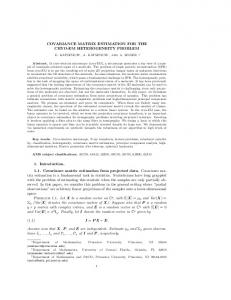
Fig. 3. Comparison of the spatial spectrum for each DOA estimation method using coprime array. � �
� where G ≡ vec ˜ a(θp1 )˜ aH (θp1 ) , vec ˜ a(θp2 )˜ aH (θp2 ) , · · · , ��
2 ˆ aH (θpKˆ ) ∈ C(M N +1) ×K , and r ≡ vec(Rs − vec ˜ a(θpKˆ )˜ 2 I) ∈ C(M N +1) ×1 . Finally, we combine the estimated σ ˆn2 ˜ source locations θ p and the enhanced power estimation (17) as � p ¯ (θ p ), θ ∈ θ p (18) p ¯ (θ) = 0, θ∈ / θp . ˆ elements in p Intuitively, only K ¯ corresponding to the estimated sources are non-zero. The combination of these two steps represents an approximation to the solution to (11). 4. SIMULATION ANALYSIS In our simulations, the coprime array consists of a pair of sparsely-spaced uniform linear arrays with M = 3 and N = 5 omni-directional sensors, respectively. It is equivalent to 2M + N − 1 = 10 physical sensor elements for the proposed DOA estimation method. The additive noise is modeled as a zero-mean white Gaussian random process. There are 12 distinct external source signals from directions uniformly distributed from −50◦ to 50◦ . The range of the angles for the predefined sparse grid is within [−90◦ , 90◦ ] with the stepsize γ = 0.1◦ between the adjacent grid points. For each simulation scenario, 1000 Monte-Carlo trials are performed. In Fig. 3, we plot the normalized spectrum of the MUSIC method for coprime array in [3], the sparse signal reconstruction method in [6] and the proposed method, with the same
1
1 0.9
Accuracy
Accuracy
0.9 0.8 0.7
Sliding Window SORTE
0.6 0.5 −10
−5
0
5
10
15
SNR(dB)
(a)
20
25
0.8 0.7 0.6 0.5 0.4
30
simulation condition SNR = 0 dB and L = 500. For fair comparison, the coprime array structure for the sparse signal reconstruction method is set to be M = 5 and N = 6, so that all of the methods conducted in the simulation are equivalent to 10 physical sensor elements. As recommended in [6], ξ = 0.25 is chosen as the regularization parameter. All of the spectra shown in Fig. 3 can identify 12 sources with only 10 physical sensor elements, therefore, the effectiveness of the coprime array for improving the DOF is verified. As depicted in Fig. 3(a), most of the responses in the spectrum are underestimated, and the spurious peaks are hard to distinguish. In Fig. 3(b), several spurious peaks appear in the sparse grid for the sparse signal reconstruction method, and the corresponding responses are relatively large and irregular, leading to the difficulty of the estimation process. In contrast, the proposed spectrum shown in Fig. 3(c) is uniformly distributed with only 12 peaks, and all of the normalized spectrum responses for each source are close to one. In Fig. 4, we compare the performance of the sliding window scheme for source enumeration to the SORTE method [15] by defining a parameter accuracy, which shows the percentage of correct source enumeration in the MonteCarlo simulations. It can be seen from Fig. 4(a) that the performance of the sliding window scheme is better than the SORTE method when SNR is larger than −5dB. The accuracy versus the number of snapshot shown in Fig. 4(b) shows that the sliding window scheme has better performance than the SORTE method. Thus, the overall performance of the sliding window scheme is better than the SORTE method. In conclusion, the comparison demonstrates that the proposed DOA estimation method can avoid spectrum leakage and achieve better spectrum performance than the other DOA estimation methods that exploit coprime arrays.
Sliding Window SORTE
100 200 300 400 500 600 700 800 900 1000
Number of snapshot
(b)
Fig. 4. Performance comparison of the sliding window scheme and the SORTE method. (a) Accuracy versus SNR with the number of snapshot L = 500, (b) accuracy versus the number of snapshot with SNR = 0dB.
2372
5. CONCLUSIONS We have proposed a DOA estimation method by covariance matrix sparse reconstruction of coprime array. The optimization problem is formulated, and the sliding window scheme is proposed for source localization. The signal power of each source is re-estimated after the DOA estimates are obtained. Simulation results demonstrate the superiority of the proposed DOA estimation method in terms of source localization, power estimation, and the achievable DOF.
6. REFERENCES [1] P. P. Vaidyanathan and P. Pal, “Sparse sensing with coprime samplers and arrays,” IEEE Transactions on Signal Processing, vol. 59, no. 2, pp. 573–586, 2011. [2] P. P. Vaidyanathan and P. Pal, “Theory of sparse coprime sensing in multiple dimensions,” IEEE Transactions on Signal Processing, vol. 59, no. 8, pp. 3592–3608, 2011. [3] P. Pal and P. P. Vaidyanathan, “Coprime sampling and the music algorithm,” in Proceedings of IEEE Digital Signal Processing Workshop and IEEE Signal Processing Education Workshop (DSP/SPE), Sedona, Arizona, USA, Jan. 2011, IEEE, pp. 289–294. [4] Z. Weng and P. M. Djuri´c, “A search-free doa estimation algorithm for coprime arrays,” Digital Signal Processing, vol. 24, pp. 27–33, 2014. [5] C. Zhou, Z. Shi, Y. Gu, and X. Shen, “Decom: Doa estimation with combined music for coprime array,” in Proceedings of IEEE International Conference on Wireless Communications & Signal Processing (WCSP), Hangzhou, China, Oct. 2013, IEEE, pp. 1–5. [6] Y. D. Zhang, M. G. Amin, and B. Himed, “Sparsitybased doa estimation using co-prime arrays,” in Proceedings of IEEE International Conference on Acoustics, Speech and Signal Processing (ICASSP), Vancouver, Canada, May 2013, IEEE, pp. 3967–3971. [7] Y. D. Zhang, S. Qin, and M. G. Amin, “Doa estimation exploiting coprime arrays with sparse sensor spacing,” in Proceedings of IEEE International Conference on Acoustics, Speech and Signal Processing (ICASSP), Florence, Italy, May 2014, IEEE, pp. 2267–2271. [8] P. Pal and P. P. Vaidyanathan, “On application of lasso for sparse support recovery with imperfect correlation awareness,” in Conference Record of the Forty Sixth Asilomar Conference on Signals, Systems and Computers (ASILOMAR), Pacific Grove, California, USA, Nov. 2012, IEEE, pp. 958–962. [9] Y. C. Eldar and G. Kutyniok, Compressed sensing: theory and applications, Cambridge University Press, 2012. [10] P. Pal and P. P. Vaidyanathan, “Correlation-aware techniques for sparse support recovery,” in Proceedings of IEEE Statistical Signal Processing Workshop, Ann Arbor, Michigan, USA, Aug. 2012, IEEE, pp. 53–56. [11] P. Pal and P. P. Vaidyanathan, “Correlation-aware sparse support recovery: Gaussian sources,” in Proceedings of IEEE International Conference on Acoustics, Speech and Signal Processing (ICASSP), Vancouver, Canada, May 2013, IEEE, pp. 5880–5884.
2373
[12] S. S. Chen, D. L. Donoho, and M. A. Saunders, “Atomic decomposition by basis pursuit,” SIAM journal on scientific computing, vol. 20, no. 1, pp. 33–61, 1998. [13] S. P. Boyd and L. Vandenberghe, Convex optimization, Cambridge University Press, 2004. [14] Y. Gu, N. A. Goodman, S. Hong, and Y. Li, “Robust adaptive beamforming based on interference covariance matrix sparse reconstruction,” Signal Processing, vol. 96, pp. 375–381, 2014. [15] K. Han and A. Nehorai, “Wideband gaussian source processing using a linear nested array,” Signal processing letters, vol. 20, no. 11, pp. 1110–1113, 2013.