3D Action Recognition and Long-term Prediction of ... - CiteSeerX

3D Action Recognition and Long-term Prediction of Human Motion Markus Hahn, Lars Kr¨ uger, and Christian W¨ohler Daimler AG Group Research Environment Perception P. O. Box 2360, D-89013 Ulm, Germany {Markus.Hahn | Lars.Krueger | Christian.Woehler}@daimler.com

Abstract. In this contribution we introduce a novel method for 3D trajectory based recognition and discrimination between different working actions and long-term motion prediction. The 3D pose of the human hand-forearm limb is tracked over time with a multi-hypothesis Kalman Filter framework using the Multiocular Contracting Curve Density algorithm (MOCCD) as a 3D pose estimation method. A novel trajectory classification approach is introduced which relies on the Levenshtein Distance on Trajectories (LDT) as a measure for the similarity between trajectories. Experimental investigations are performed on 10 real-world test sequences acquired from different viewpoints in a working environment. The system performs the simultaneous recognition of a working action and a cognitive long-term motion prediction. Trajectory recognition rates around 90% are achieved, requiring only a small number of training sequences. The proposed prediction approach yields significantly more reliable results than a Kalman Filter based reference approach. Key words: 3D tracking; action recognition; cognitive long-term prediction

1

Introduction

Today, industrial production processes in car manufacturing worldwide are characterised by either fully automatic production sequences carried out solely by industrial robots or fully manual assembly steps where only humans work together on the same task. Up to now, close collaboration between human and machine is very limited and usually not possible due to safety concerns. Industrial production processes can increase efficiency by establishing a close collaboration of humans and machines exploiting their unique capabilities. A safe interaction between humans and industrial robots requires vision methods for 3D pose estimation, tracking, and recognition of the motion of both human body parts and robot parts. To be able to detect a collision between the human worker and the industrial robot there is a need for reliable long-term prediction (some tenths of a second) of the motion. This paper addresses the problem of tracking and recognising the motion of human body parts in a working environment. The

2

Hahn, Kr¨ uger and W¨ ohler

results of action recognition are used for the long-term prediction of complex motion patterns. Our 3D tracking and recognition system consists of three main components: the camera system, the model based 3D tracking system, and the trajectory based recognition system. The input images are captured at 20 fps with a trinocular grey scale camera at VGA resolution.

2

Related Work

Previous work in the field of human motion capture and recognition is extensive, Moeslund et al. [11] give a detailed introduction and overview. Bobick and Davis [3] provide another good introduction. They classify human motion using a temporal template representation from a set of consecutive background subtracted images. A drawback of this approach is the dependency on the viewpoint. Li et al. [10] use Hidden Markov Models (HMMs) to classify hand trajectories of manipulative actions and take the object context into account. In [4] the motion of head and hand features are used to recognise Tai Chi gestures by HMMs. Head and hand are tracked with a real time stereo blob tracking algorithm. HMMs are used in many other gesture recognition systems due to their ability to probabilistically represent the variation in the training data. However, in an application with only a small amount of training data and the need for a long-term prediction of the motion, HMMs are not necessarily the best choice. A well known approach is the one by Black and Jepson [2], who present an extension of the CONDENSATION algorithm and model gestures as temporal trajectories of the velocity of the tracked hands. They perform a fixed sized linear template matching weighted by the observation densities. Fritsch et al. [6] extend their work by incorporation of situational and spatial context. Both approaches merely rely on 2D data. Hofemann [8] extends the work of Fritsch et al. [6] to 3D data by using a 3D body tracking system. The features used for recognition are the radial and vertical velocities of the hand with respect to the torso. Croitoru et al. [5] present a non iterative 3D trajectory matching framework that is invariant to translation, rotation, and scale. They introduce a pose normalisation approach which is based on physical principles, incorporating spatial and temporal aspects of trajectory data. They apply their system to 3D trajectories for which the beginning and the end is known. This is a drawback for applications processing a continuous data stream, since the beginning and end of an action is often not known in advance.

3

The 3D Tracking System

We rely on the 3D pose estimation and tracking system introduced in [7], which is based on the Multiocular Contracting Curve Density algorithm (MOCCD). A 3D model of the human hand-forearm limb is used, made up by a kinematic chain connecting the two rigid elements forearm and hand. The model consists of five truncated cones and one complete cone. Fig. 1(a) depicts the definition of

3D Action Recognition and Long-term Prediction of Human Motion

(a)

3

(b)

Fig. 1. (a) Definition of the model cones and the dependencies of the radii derived from human anatomy. (b) Extraction and projection process of the 3D contour model.

the cones by nine parameters. The 3D point p1 defines the beginning of the forearm. The wrist position p2 is computed based on the orientation of the forearm and its predefined length lforearm . The computation of the 3D point p3 in the fingertip is similar. The radii of the cones are derived from human anatomy, see Fig. 1(a) (right). As the MOCCD algorithm adapts a model curve to the image, the silhouette of the 3D model in each camera coordinate system is extracted and projected into the camera images (Fig. 1(b)). The MOCCD algorithm fits the parametric curve to multiple calibrated images by separating the grey value statistics on both sides of the projected curve. To start tracking, a coarse initialisation of the model parameters at the first timestep is required. In the tracking system we apply three instances of the MOCCD algorithm in a multi-hypothesis Kalman Filter framework. Each MOCCD instance is associated with a Kalman Filter and each Kalman Filter implements a different kinematic model, assuming a different object motion. The idea behind this kinematic modelling is to provide a sufficient amount of flexibility for changing hand-forearm motion. It is required for correctly tracking reversing motion, e.g. occurring during tightening of a screw. A Winner-Takes-All component selects the best-fitting model at each timestep. For a more detailed description refer to [7].

4

Recognition and Prediction System

The working action recognition system is based on a 3D trajectory matching approach. The tracking stage yields a continuous data stream of the 3D position

4

Hahn, Kr¨ uger and W¨ ohler

−0.16

X

1.75 −0.18

1.7 −0.2

1.65

0

5

10

15

20

25

30

35

20

25

30

35

20

25

30

35

timesteps

1.6 −0.1

1.55

Z

Y

−0.15

1.5

−0.2

1.45

−0.25

0

5

10

15

timesteps 1.4

1.75 1.7

Z

1.35 1.3 1.25 −0.25

1.65 1.6 1.55

−0.4 −0.2

−0.2 −0.15

Y

−0.1 −0.05

0

5

0 0

0.05

0.2 0.1

0.4

10

15

timesteps

X

Fig. 2. Left: 3D reference trajectories of the working action class “tightening”. Right: Time scaling (-20% (green), -10%(red), ±0% (blue), +10% (cyan), +20% (magenta)) of the blue (upper left) 3D reference trajectory. All 3D coordinates are depicted in mm.

of the tracked 3D hand-forearm limb. Our trajectories are given by the 3D motion of the wrist point p2 . A sliding window is used to match the sequence of 3D points with a set of hypotheses generated from labelled reference trajectories. 4.1

Determining the Reference Trajectories

In contrast to other previously presented approaches [3], our system relies on a small number of reference trajectories. They are defined by manually labelled training sequences. The beginning and the end of a reference action are manually determined and the resulting 3D trajectory is stored with the assigned class label. To cope with different working speeds, the defined reference trajectories are scaled in the temporal domain (from -20% to +20% of the total trajectory length) using an Akima interpolation [1]. Fig. 2 (left) shows example 3D trajectories of the working action class “tightening”. In Fig. 2 (right) time scaled reference trajectories are depicted. After labelling and temporal  scaling of the reference trajectories, we construct a set of M model trajectories m(i) , i = 1, · · · , M , which are used to generate and verify trajectory hypotheses in the recognition and prediction process. 4.2

Recognition Process

In our system the beginning and the end of a trajectory are not known a priori, which is different from the setting regarded in [5]. To allow an online trajectory matching on the continuous data stream we apply a sliding window approach which enables us to perform a working action recognition and simultaneously a long-term prediction of the human motion patterns. In contrast to the probabilistic method of [2] we deterministically match a set of pre-defined non-deformable reference trajectories (Sec. 4.1) over time and discriminate between the different classes of reference trajectories. In a preprocessing step, noise and outliers in the trajectory data are reduced by applying a Kalman Filter based smoothing process [5]. The kinematic model

3D Action Recognition and Long-term Prediction of Human Motion

5

0.5 0

1.7

−0.5 0

1.6

0.5

1.5

0

1.5

20

40

60

80

100

Y

Z

time

−0.5 0

1.4

20

40

60

80

100

time

projection on PC 1

X

1.8

1

0.5

0

1.8 Z

1.3 −0.5 0 X

0.5

−0.05

−0.15

−0.1 Y

−0.2

−0.25

1.6

−0.5

1.4 1.2 0

20

40

60 time

80

100

t

−1 0

1

2

3

4

5 6 time

7

8

9

10 11

Fig. 3. Left: Smoothed 3D input trajectory, the values in the current sliding window are red, all other blue. Middle: 3D data for each coordinate and a sliding window of length 10 frames. Right: PCA normalised data in the sliding window.

of the Kalman Filter is a constant-velocity model. Fig. 3 depicts the smoothed 3D trajectory, the current sliding window of size W = 10 frames, and the values in the sliding window normalised by a whitened Principal Component Analysis (PCA). The 3D data are projected only on the first principal component (PC 1), since the energy of the first eigenvector is always above 90%. Our sliding window approach consists of five essential operations: (i) generate trajectory hypotheses, (ii) verify hypotheses, (iii) delete hypotheses, (iv) classify remaining hypotheses, and (v) use a hypothesis for a long-term prediction of the 3D motion. Generate Trajectory Hypotheses: At timestep t we compare the current input trajectory Zt ,   Zt = (X(t−W +1) , Y(t−W +1) , Z(t−W +1) )T , . . . , (Xt , Yt , Zt )T , (1) consisting of the last W elements of the continuous data stream, with the first W elements of all reference trajectories. The compared trajectories always have the same length W and are matched with the 3D trajectory matching approach described in Sec. 4.3. The trajectory matching returns a similarity value for the two compared trajectories. If this value is smaller than a threshold Θsim the reference trajectory is assigned to the set of hypotheses and the current matching phase φ in the reference trajectory is set to (W + 1)/N . Every hypothesis is characterised by a current phase φ, 0 ≤ φ ≤ 1, within the reference trajectory of length N . The sub-trajectory, defined by phase φ and length W , aligns the model data with the current input data in the sliding window. The next essential operation is to verify the generated hypotheses and move the sliding window within the model trajectory. Verify Trajectory Hypotheses: In this step all trajectory hypotheses, generated at timestep (t − 1) or earlier, are verified. The 3D data Zt in the current sliding window is matched with the current sub-trajectory in all hypothesis trajectories. The current sub-trajectory in a hypothesis trajectory is defined by its phase φ and length W . If the 3D trajectory matching approach (Sec. 4.3) returns a similarity value smaller than Θsim , the hypothesis is kept and the current phase φ

6

Hahn, Kr¨ uger and W¨ ohler

in the model is incremented by 1/N . If a hypothesis does not pass the verification step, the no-match counter γ of the hypothesis is incremented by one. Delete Trajectory Hypotheses: This operation deletes all hypotheses for which the no-match counter exceeds a threshold ΘnoMatch . Classify Remaining Hypotheses: At timestep t we search all hypotheses which have a phase φ of more than a threshold Θrecog . If there is more than one hypothesis and different class labels are present, the no-match counter γ and the sum of all similarity values during the matching process are used to determine the winning reference trajectory. After the decision the last N elements of the input trajectory are labelled with the class label of the winning reference trajectory of total length N . Cognitive Prediction: The action recognition result is used for a long-term prediction (“cognitive prediction”). At timestep t we search all hypotheses which having a phase φ of more than a threshold Θpred . For all hypotheses found we predict the 3D position k timesteps ahead based on the underlying reference trajectory. Accordingly, the phase (φ + k/N ) in the reference trajectory is projected on the first principal component (PC 1) based on the PCA transformation of the current sliding window in the reference trajectory. This transformed value is then projected to a 3D point by applying the inverse PCA transformation of the input data Zt in the sliding window. In the case of multiple significant hypotheses, the effective prediction is given by the mean of all predicted 3D points. Typical cognitive prediction results are shown in Fig. 5. 4.3

3D Trajectory Matching

In this section we describe our 3D trajectory matching algorithm, which is used in the recognition process (Sec. 4.2) to determine the similarity between an input trajectory and a reference trajectory. Our trajectory matching approach consists of two stages: First, we compare the travelled distances along both trajectories. Then, in the second stage, we apply the Levenshtein Distance on Trajectories (LDT) to determine a similarity value. In this framework, a 3D trajectory T of length N is defined as   T = (X1 , Y1 , Z1 )T , . . . , (XN , YN , ZN )T . (2) The travelled distance T D(T) along the trajectory T is given by: T D(T) =

N X

Tt − T(t−1)

.

(3)

t=2

In the first stage we assume that two trajectories S and T are similar if the travelled distances of both trajectories T D(S) and T D(T) are similar. If S and T have a similar travelled distance they are PCA normalised and matched with the Levenshtein Distance on Trajectories (LDT). If they have no similar travelled distance the process stops at this first stage and returns the maximum length of both trajectories.

3D Action Recognition and Long-term Prediction of Human Motion

7

Normalisation: In our application we rely on a small number of reference trajectories extracted from a small number of training sequences. It is possible that the same working action is performed at different positions in 3D space, e.g. tightening a screw at different locations of an engine. Therefore the normalisation step should achieve an invariance w.r.t. translation, rotation, and scaling. Hence we apply a whitened PCA, which ensures the required invariances. Since we use a sliding window technique, the length of the matched trajectories is small, thus we project the data only on the first principal component (PC 1), defined by the most significant eigenvector, as the energy of PC 1 is always above 90 %. In the next step the trajectory based similarity measure is computed. Levenshtein Distance on Trajectories (LDT): At this point, we introduce a new similarity measure for trajectories by extending the Levenshtein distance [9]. The Levenshtein distance LD(S1 , S2 ) is a string metric which measures the number of edit operations (insert, delete, or replace) that are needed to convert string S1 into S2 . We extend this approach to d-dimensional trajectories by using the following algorithm: int LDT(trajectory S[1..d,1..m], trajectory T[1..d,1..n], matchingThresh) // D is the dynamic matrix with m+1 rows and n+1 columns declare int D[0..m, 0..n] for i from 0 to m D[i, 0] := i for j from 1 to n D[0, j] := j for i from 1 to m for j from 1 to n if(L2Norm(S[1..d,i] - T[1..d,j]) < matchingThresh) then subcost := 0 else subcost := 1 D[i, j] := min(D[i-1, j] + 1, // deletion D[i, j-1] + 1, // insertion D[i-1, j-1] + subcost)// substitution return D[m, n] 1.5 1 0.5 0

PC 1

LDT (S, T) returns the number of edit operations required to transform S into T and offers the capability to handle local time shifting. The matching threshold maps the Euclidean distance between two pairs of elements to 0 or 1, which reduces the effect of noise and outliers. Fig. 4 depicts a PCA normalised reference trajectory, an input trajectory, and the point correspondences between the trajectories. In this example the number of edit operations to transform the reference trajectory into the input trajectory is two.

−0.5 −1 −1.5

reference trajectory input trajectory

−2 −2.5

1

2

3

4

5

6

7

8

9

10

time

Fig. 4. PCA normalised reference trajectory (blue), the matching borders (dotted), a PCA normalised input trajectory (red) and the point correspondences (green) between both trajectories. The required number of edit operations is two.

8

5

Hahn, Kr¨ uger and W¨ ohler

Experimental Investigations

The system is evaluated by analysing 10 trinocular real-world test sequences acquired from different viewpoints. These sequences contain working actions performed by five different test persons in front of a complex cluttered working environment. Each sequence contains at least 900 image triples. The mean distance of the test persons to the camera system varies from 1.5m to 2m. Each sequence contains the actions listed in Table 1. All actions are performed with the right hand. The actions were shown to the test persons by a teacher in advance. All sequences were robustly and accurately tracked at virtually all timesteps with our 3D tracking system described in Sec. 3. Similar to [6] we incorporate spatial context for the actions “tightening” and “plugging”, since it is known where the worker has to tighten the screw and to place the plug and these positions are constant during the sequence. The 3D positions of the screws and holes are obtained from the 3D pose of the engine, which was determined by bundle adjustment [12] based on the four reference points indicated in Fig. 5. We utilise the following thresholds defined in Sec. 4: Θsim = 3, ΘnoMatch = 3, and Θrecog = 0.9. In the experiments we assume that if the system recognises the class “tightening” at two consecutive timesteps, the worker tightens a screw. As can be seen from Table 1, the system achieves recognition rates around 90% Action Training Trajectories (#) Test Trajectories (#) Recognised (%) tightening a screw 4 36 92 transfer motion 6 54 89 plugging 2 18 89 Table 1. Action recognition results.

on the test sequences. The recognition errors can be ascribed to tracking errors and motion patterns that differ in space and time from the learned motion patterns. Higher recognition rates may be achieved by using more training sequences, since the scaling in the temporal domain of the reference trajectories is not necessarily able to cope with the observed variations of the motion patterns. Our recognition rates are similar to those reported by Croitoru et al. [5] and Fritsch et al. [6]. Croitoru et al. use segmented 3D trajectories in their experiments, which is different from our approach. Fritsch et al. [6] rely on 2D data and their method is not independent of the viewpoint. An additional experiment was performed to determine the accuracy of the long-term prediction (k = 5, corresponding to 0.25 s). We utilise Θpred = 0.6 as a prediction threshold. As a ground truth for this experiment, we use the results of the 3D tracking system. Table 2 shows the mean and standard deviation of the Euclidean distance between the long-term prediction result and the ground truth for all test sequences. The values in Table 2 are plotted in millimetres for the proposed cognitive prediction approach and a Kalman Filter with a constantvelocity model as a reference method. As can be seen from Table 2, our longterm prediction achieves more reliable results than the Kalman Filter method. While the mean deviations are smaller about one third the random fluctuations,

3D Action Recognition and Long-term Prediction of Human Motion Name mean dist mean dist KF std dist std Kia2 61 77 32 Markus1 79 105 50 Markus2 90 118 63 Markus3 71 86 34 Stella1 63 89 33 Stella2 86 113 58 Lars1 66 81 43 Lars2 60 93 40 Christian1 67 89 35 Table 2. Long-term prediction results.

9

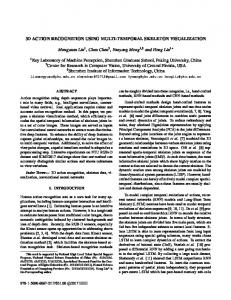
dist KF 55 94 101 64 63 106 86 88 75

(a) (b) Fig. 5. Cognitive prediction results for reversing motion (a) and transfer motion (b). In (a) and (b), the left image shows the input image at timestep t with the adapted hand-forearm model (green) and the trajectory (blue: transfer motion; red: tightening; cyan: unknown). The right image shows the image at timestep t + 5 with the ground truth position of the wrist (green cross), the cognitive prediction result (red or blue cross, depending on the action), and the Kalman Filter result with constant velocity model (yellow cross). The four linked points are reference points on the engine.

represented by the standard deviation, are reduced by a factor of about 2 by our approach. Especially for reversing motion, e.g. while tightening a screw or plugging, the proposed prediction technique is highly superior to the Kalman Filter (cf. Fig. 5).

6

Summary and Conclusion

We have introduced a method for 3D trajectory based action recognition and long-term motion prediction. Our approach allows a classification and discrimination between different working actions in a manufacturing environment. The trajectory classification relies on a novel similarity measure, the Levenshtein Distance on Trajectories (LDT). Our experimental investigations, regarding 10 long real-world test sequences, have shown that our recognition system achieves recognition rates around 90%, requiring only a small number of training trajectories. The proposed trajectory recognition method is viewpoint independent. Intermediate results of the action recognition stage are used for the long-term prediction of complex motion patterns. This cognitive prediction approach yields metrically more accurate results than a Kalman Filter based reference approach.

10

Hahn, Kr¨ uger and W¨ ohler

Future work may involve online learning of reference trajectories and the integration of HMMs, provided that an adequate number of training sequences are available.

References [1] H. Akima. A new method of interpolation and smooth curve fitting based on local procedures. Journal of the Association for Computing Machinery, 17(4):589–602, 1970. [2] M. J. Black and A. D. Jepson. A probabilistic framework for matching temporal trajectories: Condensation-based recognition of gestures and expressions. In ECCV ’98: Proceedings of the 5th European Conference on Computer VisionVolume I, pages 909–924, London, UK, 1998. Springer-Verlag. [3] A. F. Bobick and J. W. Davis. The recognition of human movement using temporal templates. IEEE Trans. Pattern Anal. Mach. Intell., 23(3):257–267, 2001. ISSN 0162-8828. doi: http://dx.doi.org/10.1109/34.910878. [4] L. W. Campbell, D. A. Becker, A. Azarbayejani, A. F. Bobick, and A. Pentland. Invariant features for 3-d gesture recognition. In FG ’96: Proceedings of the 2nd International Conference on Automatic Face and Gesture Recognition (FG ’96), page 157, Washington, DC, USA, 1996. IEEE Computer Society. [5] A. Croitoru, P. Agouris, and A. Stefanidis. 3d trajectory matching by pose normalization. In GIS ’05: Proceedings of the 13th annual ACM international workshop on Geographic information systems, pages 153–162, New York, NY, USA, 2005. ACM Press. doi: http://doi.acm.org/10.1145/1097064.1097087. [6] J. Fritsch, N. Hofemann, and G. Sagerer. Combining sensory and symbolic data for manipulative gesture recognition. In Proc. Int. Conf. on Pattern Recognition, number 3, pages 930–933, Cambridge, United Kingdom, 2004. IEEE. [7] M. Hahn, L. Kr¨ uger, C. W¨ ohler, and H.-M. Gross. Tracking of human body parts using the multiocular contracting curve density algorithm. In 3DIM ’07: Proceedings of the Sixth International Conference on 3-D Digital Imaging and Modeling, pages 257–264, Washington, DC, USA, 2007. IEEE Computer Society. doi: http://dx.doi.org/10.1109/3DIM.2007.59. [8] N. Hofemann. Videobasierte Handlungserkennung f¨ ur die nat¨ urliche MenschMaschine-Interaktion. Dissertation, Universit¨ at Bielefeld, Technische Fakult¨ at, 2007. [9] V. I. Levenshtein. Binary codes capable of correcting deletions, insertions, and reversals. Soviet Physics Doklady, 10(8):707–710, 1966. [10] Z. Li, J. Fritsch, S. Wachsmuth, and G. Sagerer. An object-oriented approach using a top-down and bottom-up process for manipulative action recognition. In DAGM06, volume 4174 of Lecture Notes in Computer Science, pages 212–221, Heidelberg, Germany, 2006. Springer-Verlag. [11] T. B. Moeslund, A. Hilton, and V. Kr¨ uger. A survey of advances in vision-based human motion capture and analysis. Computer Vision and Image Understanding, 104(2):90–126, 2006. ISSN 1077-3142. doi: http://dx.doi.org/10.1016/j.cviu.2006. 08.002. [12] B. Triggs, P. F. McLauchlan, R. I. Hartley, and A. W. Fitzgibbon. Bundle adjustment - a modern synthesis. In ICCV ’99: Proceedings of the International Workshop on Vision Algorithms, pages 298–372, London, UK, 2000. SpringerVerlag.