Aug 27, 1995 - J. Solids Structures Vol. 34, No. ...... Sutton, M., Howard, R. and Dickerson, J. (1991). ... Solution of Ill-posed Problems, John Wiley & Sons.
1m. J. Solids Structures Vol. 34, No. 16. pp. 2073- 2086, 1997 © 1997 Elsevier Science Ltd All rights reserved . Printed in Greal Brilain 0020-7683/97 $1 7.00 + .00
Pergamon
PH: 80020-7683(96)00152-7
A BOUNDARY ELEMENT SOLUTION OF AN INVERSE ELASTICITY PROBLEM AND APPLICATIONS TO DETERMINING RESIDUAL STRESS AND CONTACT STRESS F. ZHANG, A. 1. KASSAB* and D . W.NICHOLSON Department of Mechanical and Aerospace Engineering, University of Central Florida, Orlando, FL 32816, U .S.A. (Received 27 August 1995; in revisedform 10 July 1996)
Abstract-A boundary element solution is developed for an inverse elasticity problem. In this inverse problem, boundary conditions are incompletely specified. Strains can be determined experimentally, in practice, at a number of internal points and used as input to completely resolve these boundary conditions. In this paper, these strains, including random errors, are numerically simulated. This inverse problem finds applications in the evaluation of residual stress and contact stress. In contrast to previous studies, the construction of the sensitivity matrix is embedded in the boundary element formulation thereby avoiding the solution of a series of forward problems. Further, the effects of prescribed non-zero boundary conditions and body forces are included in the relation between measured strains and the primary traction unknowns. Unfortunately, the inverse problem is still ill-posed. Physical constraints are introduced to stabilize the solution. As a result, the algorithm presented here has reasonable tolerance to error in the measurement of strains. Numerical examples are given to validate the inverse algorithm. In these examples, the input strains are numerically simulated, and stable and accurate solutions are obtained with up to ± 5% random error in the input. © 1997 Elsevier Science Ltd.
INTRODUCTION
In a forward problem, the governing equation, the boundary conditions, the initial conditions, the system geometry, and the material properties are all known explicitly. The purpose of a forward problem is to resolve the field variable(s). In an inverse problem, one of the terms conventionally specified in a forward problem is not known explicitly. The purpose of the inverse problem is to determine the unknown quantity using additional information, which is usually provided by some measured data. In contrast to the solution of a forward problem, the solution of the inverse problem is generally ill-posed. The solution of general inverse problems is discussed in Tikhonov and Arsenin (1977). A review of inverse heat transfer problems can be found in Beck et a/. (1985) and more recently in Alifanov (1994). A survey of inverse problems in mechanics of materials is given in Bui (1994) . Inverse problems find wide applications in engineering analysis. In this paper, we consider a specific inverse problem which addresses the reconstruction of an unknown boundary condition in an elastostatics problem. In a forward elasticity problem, complete boundary conditions are given and responses, such as displacements, strains and stresses, need to be determined. However, in some circumstances, boundary conditions are incompletely specified, while the strains or displacements at some points in the domain of interest can be easily measured. An inverse problem can be formulated to determine the unknown boundary conditions from measured responses. Once the boundary conditions are found, the responses on the whole domain can be computed analytically or numerically. In this sense, the inverse approach is a hybrid technique. The strains or displacements can be measured on part of the boundary or inside the domain. When the displacements are measured on the boundary, over-specified boundary conditions on part of the boundary are usually used to resolve the unknown tractions on remaining part of the boundary. Another approach is to take strain or displacement * Author to whom correspondence should be addressed. 2073
2074
F. Zhang et al.
measurements at interior points in an effort to resolve the unknown tractions. In practice, internal strains can be measured without any difficulty using standard strain gages for a two dimensional plane stress problem. For a two dimensional plane strain problem or a three dimensional problem, internal strains can also be measured using embedded strainmeasuring devices, such as optical fiber sensors (Sirkis and Lo, 1994). This type of inverse elasticity problem is sometimes called the boundary condition reconstruction problem, and this is the inverse problem considered in this paper. Maniatty et al. (1989) studied the boundary reconstruction inverse problem using the finite element method (FEM). Schnur and Zabaras (1990) introduced a 'spatial smoothing' technique and a 'key node' method in their FEM solution of the inverse problem. Zabaras et al. (1989) presented a solution to the inverse problem for given internal displacement measurements using an integral approach. Yeih et al. (1993) proposed a regularized solution to the inverse problem for overspecified boundary conditions. Zhang et al. (1994, 1995) studied the inverse problem for given internal strain measurements using the boundary element method (BEM). Recently, Bezerra and Saigal (1995) developed a BEM based optimization method with analytical evaluation of the gradient of the objective function for the solution of the inverse problem at hand. Martin et al. (1995) developed a BEM based algorithm for the reconstruction of unknown boundary tractions. They use overspecified boundary conditions on a portion of the boundary and singular value decomposition to solve the problem. The solution of this inverse problem finds direct application in determining contact stress between elastic bodies, Kihara et al. (1983) and ada and Shinada (1987). Another application of this inverse problem is related to determination of residual stress in structural components. Kihara (1983) calculated residual stress in a plate from stress changes during cutting processes by the inverse approach. Veda et al. (1975) and Rybicki et al. (1988) employed a similar method in studying the material removal method for residual stress measurement. Zhang et al. (1994) also studied this application of the inverse problem using BEM. In this paper, we develop a BEM solution to the boundary condition reconstruction problem using internal strain measurements as additional inputs. Our algorithm features three important components. First, the calculation of the sensitivity matrix, which relates boundary unknowns to strain measurements, is embedded in the BEM formulation. Consequently, the computational effort is significantly reduced in comparison to finite element solutions, Schnur and Zabaras (1990), and previous BEM solutions, Zhang et a/. (1994). In particular, the computational burden is reduced to the formation of four BEM influence matrices and the appropriate rearrangement of partitions of the influence matrices. This is in sharp contrast to previous approaches which require a series of forward solutions to construct the sensitivity matrix. Second, the effects of prescribed non-zero boundary conditions and body forces are included in the relation between measured strains and the primary traction unknowns. This general relation is critical in many practical applications. For instance, in rolling problems, the effect of the weight of the roller is obviously of importance and must be accounted for. Third, in addition to aforementioned features of our algorithm, global equilibrium conditions are introduced as additional constraints to improve numerical stability and enforce compliance to fundamental physical principles. These constraints are adjoined through the use of Lagrange multipliers to the least squares functional which measures the difference between computed and input strains in the L2 norm. Numerical examples are presented to validate our inverse algorithm. In these examples, input strains are numerically simulated, and stable and accurate solutions are obtained using strains with as much as ± 5% random error. INVERSE PROBLEM AND ITS APPLICATIONS
Consider the two dimensional elastic body n shown in Fig. 1. The boundary r of n consists of three parts: rJ, r 2 , r 3 , with prescribed displacements u\ on rJ, prescribed tractions t2 on r 2 , and both displacements U3 and tractions t3 as unknowns on r 3 • Strains
A boundary element solution of an inverse elasticity problem
2075
are measured at several internal points close to r 3 . The inverse problem is to determine t3 from the measured strains. After determining t3 , one can further solve for displacements, strains and stresses over the whole domain through a forward analysis. Since only linear elasticity is considered here, the measured strains can be related to t3 in matrix form using the following superposition:
{e} = [C]{t3} + {b} + {d}.
(1)
The matrix [C] is called the sensitivity matrix and has dimension M x N, where M and N are the number of measured strains and the number of unknown traction components on r 3, respectively. Vector {b} accounts for internal strains due to prescribed displacements Ul on r 1 and prescribed tractions t2 on r 2, and vector {d} accounts for internal strains due to body forces. Once matrix [C] and vectors {b} and {d} are formulated, {t3} can be determined from strain measurements. It should be noted that, by including the vectors {b} and {d}, eqn (1) is a general relation, explicitly accounting for body forces and specified nonzero boundary conditions. Application to evaluation of contact stress
The contact problem is usually difficult to solve analytically or even numerically, especially when plastic deformation is involved. To simplify the calculation, different contact models are assumed, such as perfect bonding contact or sliding contact, frictional contact or frictionless contact. However, a physical problem usually cannot be simulated with a single contact model, and, often, a combination of models is required. On the other hand, direct measurement of the contact stress is often impossible because of the inaccessible nature of the interface. To avoid these difficulties, an inverse approach can be employed to resolve the contact stress on r3 based on experimental measurements of internal displacement or strain. Since the contact area is not always known in advance, a potential contact area, which should be large enough to cover the actual contact area, is assumed. The actual contact area can be easily found after the traction distribution is resolved. The zero traction area indicates non-contact locations. Application to residual stress measurement
Residual stress is self-balanced stress locked in an object without the application of external loads. As a result, it is necessary to relieve residual stress, by cutting or machining for example, in order to measure it by conventional experimental stress analysis. Residual stress along the cutting plane prior to cutting can be computed from measurement of the
13(u~,t~) * * * * * * * * * * *
* ., *
11 (u~,t~)
u-unknown k-known * - measuring points
Fig. I. Definition of the inverse problem.
0
2076
F. Zhang et al. / / /
0
/0 / /
0
--Measuring points
II
+
resiciual stress ciis t r ibution
Fig. 2. Application to residual stress evaluation.
ensuing deformation by solving an inverse problem. This residual stress relieving process can be regarded as applying an opposite load to the cutting plane of the original object, see Fig. 2. Kihara et al. (1983) calculated the residual stress field in a plate from stress changes during cutting. However, in their numerical simulation, no errors in the measurements are considered and therefore the tolerance of their method to measurement errors remains unknown.
FORMULATION OF THE SENSITIVITY MATRIX
In FEM solutions, Schnur and Zabaras (1990), and previous BEM solutions, Zhang et al. (1994), the 'unit load' method was used to compute the elements of the sensitivity matrix [C] in eqn (1). In this method, a single unit traction component is applied at one boundary node each time, and strain values at measuring points are obtained through a forward analysis. These values give one column of the sensitivity matrix. Using this approach, a total of N forward analyses are required to obtain the matrix. When the number of unknown traction components on 13 is large, a considerable amount of computations is needed. In contrast to the 'unit load' method, the formation of [C], {b} and {d} in this paper is embedded in the BEM formulation, thereby avoiding a series of forward analyses. Consequently, a brief review of the BEM followed by an outline of our approach to the formulation of [C], {b}, and {d} is given below. Somigliana's identity provides an expression for internal displacement Ui(~) in terms of boundary traction tk(x) and boundary displacement Uk (x) as:
where ~ is any point in the domain, fl, x lies on domain boundary, 1, and z is within the domain, fl. The body force is denoted by bk • The tensors u;t and t;t are fundamental solutions for displacements and tractions, respectively, and can be found in standard BEM texts (e.g. Brebbia et al., 1984). In eqn (2), the domain integral appears only if the distributed body force terms, bk> are important in the analysis of the problem at hand. By differentiating the above expression for displacements, strains cfln be expressed as follows:
A boundary element solution of an inverse elasticity problem
2077
where U~;k and t,;k are strain kernels and can be derived from the fundamental solutions. After discretizing the boundary and interpolating displacements and tractions within each element, the above two integral relations can now be written in the following discretized form: Ui(~)
eij(~)
= =
2K
2K
k~O
k~O
L Giktk + L Hikuk+!;
2K
2K
k~O
k~O
L Eijktk - L FijkUk+gij
(4)
(5)
where K is the number of boundary nodes. Writing eqn (4) for all boundary points and applying eqn (5) for all M-internal measuring points, one can get the following two equations in matrix form : [H]{u} = [G]{t} + {f}
(6)
{s} = [E]{t}-[F]{u}+{g}
(7)
where {u} is the vector of nodal displacements and {t} is the vector of nodal tractions. Matrices [H] and [G] have dimension 2K x 2K and matrices [E] and [F] have dimension M x 2K. The evaluation of [H] and [G] matrices and the body force terms, {f} and {g}, is carried out numerically using the standard BEM, see Banerjee (1994). Further, it is noted that the formulation of [E] and [F] matrices presents no singularity since all the measuring points are internaL Rewriting the above two equations to accommodate the specified boundary conditions leads to :
[HI
H2
{s} = -[FI
H{}[G' G{}{f) G2
F, F{}[E. E, E{}{g)
(8)
(9)
Up to this point, the standard BEM formulation has been used. We now show that matrix [C] and vectors {b} and {d} in eqn (1) can be expressed explicitly in terms of components of the above mentioned four matrices and known boundary conditions. Since t3 is the primary unknown in the inverse problem, it is essential to separate t3 from other unknowns. Moving {q and all known boundary conditions to the RHS and all other unknowns to the LHS in eqn (8) results in :
(10)
or
F. Zhang et al.
2078
(11)
where {x} = (II U2 U3? is an unknown vector, {bI} is a known vector. The unknown vector {x} can then be expressed in terms of {q and known quantities as follows:
{x} = [A]-I[G 3]{t3} + [A]-I {bd +[A]-I {f})
= [G;]{t3}+{b'd+{f'}.
(12)
Rearranging eqn (9) similarly, the internal strains can be expressed as follows:
or (14) where [F'] = [ - EI F2 F 31, {b2 } is a known vector. Substituting eqn (12) into (14) yields an expression in the form of eqn (1). In particular, we arrive at:
{8} = ([E31 - [F'][G;]) {t3} +({b 2} - [F']{b'I })+({g} - [F']{f'}) =
[CHt 3 } + {b} + {d}
(15)
where [C] = [E3] - [F'][G;]
{b} = {b 2 }
{d}
=
-
[F'] {b'I}
(16)
{g} - [F']{f'}.
Equation (16) provides explicit expressions for matrix [C] and vectors {b} and {d}. Thus, the main difference between eqn (15) and eqn (9), which is the standard strain expression using integral relations, is that the appropriate rearrangement of eqn (8) is incorporated into eqn (9) in order to arrive at the explicit relations for the sensitivity matrix and the vectors reflecting the effects of prescribed boundary conditions and body forces. Minimal effort is needed to implement this formulation in an existing BEM code. If body forces are negligible for the problem under consideration, the tasks involved are the generation of the four influence matrices [H], [G], [E], and [F], their appropriate partitioning and rearrangement as outlined above, the inversion of the matrix [A], and some numerical matrix operations. It can be seen that sensitivity matrix [C] and vectors {b} and {d} can be formed simultaneously with the amount of computations comparable to a single BEM forward analysis. This has been verified in our numerical computations. This is in sharp contrast to the common practice of calculating [C] by the 'unit load' method which requires N-BEM solutions. If the body forces are significant, the vector {d} can then be formed as given in eqn (16). CONSTRAINED LEAST-SQUARES MINIMIZATION
The unknown vector {t3} is related to the strain measurements through the sensitivity matrix [C], as shown in eqn (1). Numerical analysis shows that the actual traction distribution can be resolved by solving (1) provided the strain inputs are exact and M is equal to N. However, when there is a small amount of error in the strain input, solving eqn (1) directly usually gives meaningless results. This is because not all the measurements are
A boundary element solution of an inverse elasticity problem
2079
independent, and, as a result, the sensitivity matrix [C] is nearly singular. Instead, improved results can be obtained using a least-square method to minimize the difference between the measured strains and the calculated strains. This allows the number of measurements M to be greater than the number of unknowns N. Even in this overdetermined case, the solution may still lead to an unreasonable answer. To overcome this numerical sensitivity, Schnur and Zabaras (1990) introduced "spatial regularization" to impose some smoothing conditions on the unknown variables. The smoothing effects depend on the order of the regularization and the choice of smoothing parameters. These are difficult to determine a priori.
The introduction of quantitative constraints is another way to improve tolerance to errors in input data, as noted by Sutton (1991) and Schnur and Zabaras (1990). Prescribed traction values at specific points (e.g. zero traction points) are used as constraints both in Sutton (1991) and Schnur and Zabaras (1990). However, this type of constraint is usually unavailable in practical applications. In this work, we propose another kind of constraint in the form of equilibrium conditions. In the solution of a forward elasticity problem, the global equilibrium conditions are automatically satisfied. However, in an inverse problem, due to error in measurements, resolved boundary tractions do not satisfy these conditions in general. Therefore, it is necessary to apply these equilibrium conditions as additional constraints. A counterpart of these equilibrium constraints, in the form of conservation of energy, has been used and found to be important in the solution of the inverse heat conduction problem, Das (1991). The global equilibrium conditions can be expressed in the following form:
r ty dr = 12
Jr
3
r (tyx-txy)dr = 1
Jr
3,
(17)
3
The determination of constants II> 12 and 13 depends on the problem to be solved. In some cases, these constant are simply zero. For example, in the case of residual stress, II> 12 and 13 are zero due to the self-equilibration of the residual stresses. For the contact problem which involves an elastic body included in another elastic body, as shown in Fig. 3, the three constants must also be zero in order to keep the internal body in equilibrium. However, often these constants are not zero, but equal and opposite to the sum of the forces (/1 and 12 ) and the moments (/3) acting on the remaining portion of the domain of interest. For instance, in the plate contract analysis of example 3 shown in Fig. 9, the constants are determined from the fact that the integrated force acting on the upper plate is balanced by the contact pressure at the bottom from the bottom plate. However, as will be shown in the example section, symmetry is invoked in the BEM analysis of this problem; consequently, the moment constraint is explicitly enforced and thus redundant, in this particular example. The discretized forms of these constraints are:
{DdT {t3} = II {Dd T{t3} = 12 {D3V {t3} = 13 , Equation (18) can be written in the following matrix form:
(18)
2080
F. Zhang et al.
Fig. 3. Demonstration of the determination of constraint constants for contact problems.
(19)
The matrix [D] is determined only by the problem geometry and discretization used in the analysis. For example, matrix [D] takes the following simple form for a constant element model with fixed element lengths:
[D] =
[~
o
Yl
1
o
o
1
o
(20)
Yn
where x/s and y;'s are coordinates of the boundary element nodes. For higher order elements, [D] takes a more complicated form and can be evaluated either analytically or numerically. The following constrained least-square minimization can now be defined to solve the inverse problem: Find to minimize subjectto
{t3} ([C]{t3} + {b} + {d} - {8})T([C]{t3} + {b} + {d} - {8}) [D]{t3} = {I}.
The least squares functional measures the difference between computed and input strains in the L2 norm, while the constraints enforce global equilibrium. Lagrange multipliers are used to adjoin these constraints to the functional, and the augmented functional is introduced as:
(21)
Differentiating F with respect to {t3} and Ai and setting the result to zero gives the following constrained normal equations in matrix form:
2081
A boundary element solution of an inverse elasticity problem
I
[C]T[C]
{Dd
{DdT
o o o
{D2}T
{D3V
(22)
Numerical experimentation further reveals that the condition number of the system matrix of eqn (22) is much smaller than that of eqn (1). Therefore, the solution of eqn (22) is less sensitive to the error in the measurements than the solution of eqn (1). This indicates that the introduction of physical constraints has the desired effect of stabilizing results and guiding the calculated traction toward the exact one. It should be noted that, in the process of stabilizing the normal equations, these constraints enforce adherence to fundamental physical principles. NUMERICAL RESULTS
Three numerical examples are given in this section to validate the solution procedure developed in the preceding sections. The strain input to the inverse problem is simulated by a BEM forward analysis. To model measurement error, strains with up to ± 5% random error are used as input in the inverse solution. In all cases, quadratic isoparametric boundary elements are used, and constraint equations in eqn (19) are also evaluated using quadratic shape functions. In the first example, a case is studied where specified nonzero tractions are applied on portions of the boundary, thus {b} #- 0 in eqn (15). In the remaining two examples {b} = O. The effect of the location of measuring points on the inverse solution was discussed in a previous study (Zhang et al., 1994) and will not be addressed in the following examples. Example 1 A square plate is considered in this example. The boundary conditions are shown in Fig. 4(a). The linearly distributed normal traction on the right side surface is known, and the normal traction on the top surface is the primary unknown. Thus, {b} must be evaluated in this case. The tangential traction on the top surface is assumed to be zero. Strains are known at three points shown in Fig. 4(b), and are used to determine the unknown traction distribution on the top surface. Figure 4(b) also shows the BEM model, which consists 16 quadratic elements. The computed traction distribution from exact strain input is shown 32
""
Fig. 4. Example 1.
A
A I
\ \
I \
I
f'lE'o.suring points
/
,I
2082
F. Zhang et al. 350
300
-
250
Exact Traction • Computed Traction
200
1SO
c 0
:g ....!'!
100 SO
0 3
4
5
7
-SO -100 -1 SO -200
X Fig. 5. Computed normal traction from exact input strains.
in Fig. 5, and the exact solution is recovered. Random numbers are then generated within the range of ± 5% of the exact strain, and they are added to the exact strains to simulate measurement errors. The exact strains and the strains with errors are given in Table 1. The unknown traction is then resolved using strains with simulated errors. Results are plotted in Fig. 6 for two cases: with and without enforcement of physical constraints. Clearly, results obtained without constraints are meaningless, while those obtained with constraints are fairly close to the exact data. This clearly demonstrates the effect of the constraints in stabilizing the solution of the inverse problem, and validates our formulation of the nonzero boundary condition vector {b}. Example 2 The same plate as in example 1 with different traction boundary conditions is studied in this example. In addition to the normal traction, there are tangential tractions on the top surface of the plate, as shown in Fig. 7. Both normal and tangential tractions are assumed to be unknowns and need to be resolved from strain measurements at nine points. This example can be regarded as a simulation of measurement of residual stress along a cutting plane. With exact input strains, exact traction distribution is again obtained and needs not to be reported. Computed tractions obtained using the proposed solution procedures and input strains with up to ± 5% random error are plotted in Fig. 8. Both computed normal traction and computed tangential traction are in good agreement with the exact distributions. Table 1. Exact strains and strains with ± 5% random error in Example 1 (strains are obtained by assuming E = 1) Exact strain £ -0.04940 -0.00575 -0.03867 -0.02956 -0.10227 0.01204 0.00211 -0.02895 0.05339
Random number between [-5, 5] e
Strain with error £(1- e%)
3.170 -2.845 -2.165 2.205 -1.181 1.060 -4.435 0.691 4.140
-0.04783 -0.00591 -0.03951 -0.02891 -0.10348 0.01191 0.00221 -0.02875 0.05118
A boundary element solution of an inverse elasticity problem
2083
600 500
- - Exact Traction ..•.. Computed Traction with Constraints -+-Computed Traction without Constraint
400 300
200
c 0
:;::J
100
u
!!
~
0
7 -100
-200 .3OQ
-400 -500
X Fig. 6. Computed normal traction from input strains with up to
± 5% random error.
norMol troction
tongentiol troction
/
Fig. 7. Example 2.
2084
F. Zhang et al. 100T-----------~--~--------------------------------------__,
so
0 3
2
5
6
7
Tx
-SO
-100 -1SO
---Exact X-traction ..•.. Computed X-traction
.1-______________________________________________________- - - '
350 300 250
- - - Exact Y-traction ..•.. Computed Y-traction
200 150 100 Ty
SO 0 3
4
5
7
-SO -100 -150 -200
Fig. 8. Computed normal and tangential traction from input strains with up to
± 5% random error.
Example 3 The measurement of contact stress between two plates is simulated in this example. The contact stress given by Chen and Chen (1992) is used to specify strain input at measuring points. Frictionless contact is assumed in this example for convenience. Because of symmetry, only half of the structure is modeled using BEM, as shown in Fig. 9. Since the exact contact area is not known in advance, the area covered by the top plate is assumed to be the potential contact area. There are 26 quadratic elements and 11 traction unknowns in this example. Strains at five measuring points are used as input to the inverse problem. The constraints introduced here have the effect of keeping the top plate in equilibrium. Numerical results show again that simply solving eqn (1) does not reproduce the given contact stress distribution. Plotted in Fig. 10 is the result from the proposed inverse solution with explicit enforcement of the physical constraints. The contact stress is accurately retrieved. From the computed contact stress distribution, it is easy to determine that the actual contact area extends 15 cm away from the center line.
2085
A boundary element solution of an inverse elasticity problem
p
il
-!lr--
T
,
I·
2 .O
·1
5~0 I
I
1 30.0
I
I,
~
7~0 Fig. 9. Example 3.
140 120 - - Exact Contact Stress
100
~
U5
80
-0
60
U
40
.l!l c:: a
..•.. Computed Contact Stress
20 0 2.5
5
7.5
10
12.5
15
17.5
20
22.5
-20 X Fig. 10. Computed contact stress.
CONCLUSIONS
A boundary element solution is developed for an inverse elasticity problem whose purpose is to reconstruct an unknown boundary condition using internal strain measurements as inputs. The calculation of the sensivitity matrix is embedded in the BEM formulation, and, therefore, the computational effort is significantly reduced compared to previous studies. Further, by including the effects of prescribed non-zero boundary conditions and body forces, the relation between measured strains and the primary traction unknowns used in this paper is general. Constrained least-square minimization is used to solve the inverse problem. In contrast to other regularization methods, the constraints introduced here have clear physical meaning. In all numerical examples, the proposed inverse solution reproduces the exact stress distribution with reasonable accuracy. All input used in the numerical examples consists of numerically simulated strains superimposed with up to ± 5% random error. Corresponding experimental work is under way and will soon be reported.
2086
F. Zhang et al. REFERENCES
Alifanov, O. M. (1994). Inverse Heat Transfer Problems, Springer-Verlag, New York. Banerjee, P. K. (1994). Boundary Element Methods in Engineering, McGraw-Hill, New York. Beck, 1. V., Blackwell B. and St. Clair, Jr., C. R. (1985). Inverse Heat Conduction: Ill-Posed Problems, WileyInterscience, New York. Bezerra, L. and Saigal, S. (1995). Inverse boundary traction reconstruction with BEM. International Journal of Solids and Structures 32, 1417-1431. Brebbia, C. A., Telles, J. C. F. and Wrobel, L. C. (1984). Boundary Element Techniques, Springer-Verlag, New York. Bui, H. D. (1994). Inverse Problems in the Mechanics of Materials: An Introduction, CRC Press, Boca Raton. Chen, W. H. and Chen, T. C. (1992). Boundary element analysis for contact problems with friction. Computers and Structures 45, 431-438. Das, S. (1991). Numerical solution of inverse problems in mechanics using the boundary element method. Ph.D. dissertation, Iowa State University. Kihara, J., Shen, G., Yamauchi, T., Mimura, H., Makino, H. and Liu, B. (1983). Some applications ofBEM for evaluation of the deformation of the tool and the calculation of the residual stress distribution in the product in the plastic working process. In Proc. 5th Int. Con! Boundary Elements (eds C. A. Brebbia et al.), pp. 393405, Hiroshima, Springer-Verlag, New York. Maniatty, A., Zabaras, N. and Stelson, K. (1989). Finite element analysis of some inverse elasticity problem. Journal of Engineering Mechanics ll5, 1303-1317. Martin, T., Halderman, J. and Dulikravich, G. (1995). An inverse method for finding unknown surface traction and deformations in elastostatics. Computers and Structures 56, 825-835. Oda, J. and Shinada, T. (1987). An inverse analysis technique to obtain contact stress distribution. Transactions of the JSME53, 1614-1621. Rybicki, E., Shadley, J., Sandhu, A. and Stonesifer, R. (1988). Experimental and computational residual stress evaluation of a weld clad plate and machined test specimens. Journal of Engineering Materials and Technology llO, 297-304. Schnur, D. S. and Zabaras, N. (1990). Finite element solution of two dimensional inverse elastic problems using spatial smoothing. International Journal of Numerical Methods in Engineering 30, 57-75. Sirkis, 1. S. and Lo, Y-L. (1994). Simultaneous measurement of two strain components using 3 x 3 and 2 x 2 coupler-based passive demodulation of optical fiber sensors. IEEE Journal of Lightwave Technology 12, 21532161. Sutton, M., Howard, R. and Dickerson, J. (1991). A constrained least square approach for hybrid stress analysis of elastic bodies. Engineering Analysis 8,58-67. Tikhonov, A. N. and Arsenin, V. Y. (1977). Solution of Ill-posed Problems, John Wiley & Sons. Ueda, Y, Fukuda, K., Nakacho, K. and Endo, S. (1975). A new measuring method of residual stress with the aid of finite element method and reliability of estimated values. Transactions of the JWRI (Welding Research Institute of Osaka University, Japan) 4, 19-27. Yeih, W., Koya, T. and Mura, T. (1993). An inverse problem in elasticity with partially overprescribed boundary conditions, Part I : Theoretical approach. Journal of Applied Mechanics 60, 595-600. Zabaras, N., Morellas, V. and Schnur, D. (1989). Spatially regularized solution of inverse elasticity problem using the BEM. Communications in Applied Numerical Methods 5,547-553. Zhang, F., Kassab, A. J. and Nicholson, D. W. (1994). Application of the boundary element method to meaasurement ofresidual stress. In BETECH IX (eds C. A. Brebbia and A. J. Kassab), pp. 165-172, Computational Mechanics Publications, Boston. Zhang, F., Kassab, A. J. and Nicholson, D. W. (1995). A boundary element inverse approach for determining residual stress and contact pressure. In Boundary Elements XVII (eds C. A. Brebbia et al.), pp. 331-338, Computational Mechanics Publications, Boston.