A Comparison of Synthesis Methods for Cellular Structures ... - EDGE
Recommend Documents
University of Wolverhampton 2004. All rights reserved. No part of this work may be reproduced, photocopied, recorded, stored in a retrieval system or transmitted ...
applications such as heat exchangers or catalyst support structures. ... hexagonal periodic cellular structures on heat transfer and pressure drop. Finite element ...
e-mail: [email protected]. M. R. Herson. Medical School, Micro and ..... and Energetic Research Institute â. IPEN, SaËo Paulo, 124 p. http://www.teses.usp.br/teses/.
ABSTRACT. This paper presents a comparison of different methods for noise reduction in Behind-The-Ear (BTE) hearing aids with two microphones. In this work ...
4 - Objects (csph, torus, sombrero, cube, sphere and noisedsph) .... The position difference for a sombrero object was slightly smaller and similar to the results.
CLIMBING PERFORMANCE by. Colin Matthew .... Commonly-Used Dependent
Measures in Climbing Research. ... Training for Rock Climbing Performance .
problems: stock outs and surplus stock. The con- sequence of stock outs is lost sales, and potentially lost customers. Surplus stock results in added hold- ing cost ...
Page 1 ... Abundance Determinations in K-Type Stars. L. Affer1, G. Micela1, ... faults. The two spectroscopic methods give consistent results suggesting that non-.
Mar 30, 2016 - able to use the blind test interface to detect PD at a clinic or remote location .... pushbutton at the bottom of the all data application and blind test screens. ..... Oung, Q.W.; Muthusamy, H.; Lee, H.L.; Basah, S.N.; Yaacob, S.; ...
Kun-Ho Seo a,*. aCollege ... Conclusion: The results of this study suggest that rep-PCR provided the best .... and Inspection Agency (Anyang, South Korea). 2.3.
Oct 15, 2014 - exchangeable with other cations in the soil solution and are readily ... Thus, CEC is important for maintaining adequate quantities of plant available ... In one of these methods [13, 14] the exchangeable cations are extracted with ...
Disease Revision 10 Canadian Enhancement (ICD10-CA) codes. These codes ... tistics Canada Health Region Boundary File18 and Postal Code Con-.
2 Livingstone v Rawyards Coal Co [1880] 5 App. Cas. 25 p. 39. ..... for age intervals though this is at the cost of less accurate estimates. The alternative is.
Samples were optically characterized as a function of wavelength. A brief ... comparison between the optical properties of the samples returned by the different ...
With each hearing aid a two-stage adaptive beamformer (A2B) can be added. To make a comparison between different methods (HAO, HA2D, HA3D, HA1+A2B,.
Jul 7, 2010 - Specifically, the degree of denaturation of whey proteins is thought ...... researchers and the Cal Poly creamery would not be using the cheese ...
708. SCALING BY ENTROPY MAXIMIZATION. References. COLLINS, D. M. (1982). Nature (London), 298, 49-51. Fox, G. C. & HOLMES, K. C. (1966). Acta Cryst.
E. Bauer, C. Pennerstorfer, P. Holubar, C. Pias and R. Braun. Institute ofApplied ... that this initial respiratory response, recorded before any growth of the existing.
Dilutions of sera (1:64, 1:128, and 1:256, etc., for IgG and 1:16 and 1:32 for IgM) and of CSF (undiluted, 1:2, and 1:4, etc., for. IgG and IgM) were overlaid onto ...
These include thermal effects, which can potentially flip the state of a cell. Small clocking zones allow the designer the ability to create more complicated. Fig. 2.
Honda's Odyssey, the minivan sales leader1, returns a carryover for 2015 with a
modest price increase after undergoing ... Blu-ray Rear Seat Entertainment
together with Navigation on more trims throughout its lineup ... Heated front seats.
Abstract - We present and compare five approaches for synthesizing and relighting real 3D surface textures. We adapted Efros's texture quilting method and ...
Jan 28, 2007 - systems of nonlinear ordinary differential equations (ODEs). ... N-1325 Lysaker, Norway; email: [email protected]; email: [email protected];.
A Comparison of Synthesis Methods for Cellular Structures ... - EDGE
A Comparison of Synthesis Methods for Cellular Structures with Application to Additive ..... Target deflections of nodes at the free end are determined as 20 percent of the .... objective function calls, compared to 10,050 calls required by PSO.
A Comparison of Synthesis Methods for Cellular Structures with Application to Additive Manufacturing
Jane Chu, Sarah Engelbrecht, Greg Graf, David W. Rosen The George W. Woodruff School of Mechanical Engineering, Georgia Institute of Technology, Atlanta, GA 30332-0405 404-894-9668, [email protected] Abstract Cellular material structures, such as honeycombs and lattice structures, have been engineered at the mesoscale for high performance and multifunctional capabilities. We desire efficient algorithms for searching the large, complex design spaces associated with cellular structures. In this paper, we present a comparison of two synthesis methods, Particle Swarm Optimization (PSO) and least-squares minimization (LSM), for the design of components comprised of cellular structures. Computational characteristics of the algorithms are reported for design problems with hundreds of variables. Constraints from SLS and direct-metal manufacturing processes are incorporated to ensure that resulting designs are realizable. Two 2dimensional examples are used to study the characteristics of the proposed synthesis methods. Keywords: cellular materials, lattice structures, design synthesis, particle swarm optimization, least squares minimization, additive manufacturing. 1
INTRODUCTION
1.1
Cellular Materials The concept of designed cellular materials is motivated by the desire to put material only where it is needed for a specific application. From a mechanical engineering viewpoint, a key advantage offered by cellular materials is high strength accompanied by a relatively low mass. These materials can provide good energy absorption characteristics and good thermal and acoustic insulation properties as well [8]. Cellular materials include foams, honeycombs, lattices, and similar constructions. When the characteristic lengths of the cells are in the range of 0.1 to 10 mm, we refer to these materials as mesostructured materials. Mesostructured materials that are not produced using stochastic processes (e.g. foaming) are called designed cellular materials. In this paper, we focus on designed lattice materials.
459
In the past 10 years, the area of lattice materials has received considerable attention due to their inherent advantages over foams in providing light, stiff, and strong materials [2]. Lattice structures tend to have geometry variations in three dimensions; some of our designs are shown in Figure 1. As pointed out in [6], the strength of foams scales as ρ1.5, whereas lattice structure strength scales as ρ, where ρ is the volumetric density of the material. As a result, lattices with a ρ = 0.1 are about 3 times stronger than a typical foam. The strength differences lie in the nature of material deformation: the foam is governed by cell wall bending, while lattice elements stretch and compress. The examples in Fig. 1 utilize the octet-truss (shown on the left), but many other lattice structures have been developed and studied (e.g., kagome, Kelvin foam). We have developed methods for designing lattice mesostructure for parts [17,20] and have developed design-for-manufacturing rules for their fabrication in SL. Methods of continuum mechanics have been applied to various mesostructured materials. Ashby and co-workers wrote a book on metal foam design and analysis [2]. They and others have applied similar methods to the analysis of lattice structures. The octet truss in Fig. 1 has been extensively analyzed. Deshpande et al. [6] treated the octet truss unit cell as a collection of tension-compression bars that are pin-jointed at vertices and derived analytical models of their collapse behavior for many combinations of stresses. Their results match finite element model behavior well, but tend to under-predict the strength and stiffness of octet trusses due to their assumption of pin-jointed vertices. Wang and McDowell [21] extended this study to include several other lattice cells. Recently, we have been developing a more general analytical model of lattice behavior [11]. From our general model, models for octet and other lattice structures can be derived. We base our model on a single vertex with a collection of struts incident on that vertex. This vertex model will be our base “unit cell” for representation and modeling purposes.
1
0.5
0
d
w
d
1
b) skin with single layer of lattice structure
w 0.5
v
u 0 0
u
0.5
1
v
a) octet-truss
c) Skin with 2 layers of truss structure made in SL
Figure 1. Octet-truss unit cell and example parts with octet-truss mesostructures. 1.2
Design for Additive Manufacturing Design for manufacturing (DFM) has typically meant that designers should tailor their designs to eliminate manufacturing difficulties and minimize costs. However, the improvement of rapid prototyping, or Additive Manufacturing (AM), technologies provides an opportunity to re-think DFM to take advantage of the unique capabilities of these technologies. Several companies are now using AM technologies for production manufacturing. For example,
460
Siemens, Phonak, Widex, and the other hearing aid manufacturers use selective laser sintering (SLS) and stereolithography (SL) machines to produce hearing aid shells, Align Technology uses stereolithography to fabricate molds for producing clear braces (“aligners”), and Boeing and its suppliers use SLS to produce ducts and similar parts for F-18 fighter jets. In the first three cases, AM machines enable one-off, custom manufacturing of 10’s to 100’s of thousands of parts. In the last case, AM technology enables low volume manufacturing and, at least as importantly, piece part reductions to greatly simplify product assembly. More generally, the unique capabilities of AM technologies enable new opportunities for customization, improvements in product performance, multi-functionality, and lower overall manufacturing costs. These unique capabilities include: • • •
Shape complexity: it is possible to build virtually any shape, lot sizes of one are practical, customized geometries are achieved readily, and shape optimization is enabled. Material complexity: material can be processed one point, or one layer, at a time, enabling the manufacture of parts with complex material compositions and designed property gradients. Hierarchical complexity: hierarchical multi-scale structures can be designed and fabricated from the microstructure through geometric mesostructure (sizes in the millimeter range) to the part-scale macrostructure.
In this paper, we are interested in developing design methods that enable designers to take advantage of the shape complexity capabilities of AM processes. Specifically, we develop design synthesis methods for cellular materials in general, and lattice structures in particular [17]. We first present a problem formulation for general structural synthesis applications (Section 2). In Section 3, we propose two synthesis algorithms, Particle Swarm Optimization and Least Squares Minimization, that show promise in searching the design spaces defined in our problem formulation. Two examples are investigated in Section 4 and the performance of the synthesis algorithms is compared. 2
PROBLEM FORMULATION The class of problems being solved is most closely related to size optimization, although our problems have aspects of topology optimization and multiobjective decision making. Given the synthesis methods under investigation, we use unconstrained problem formulations, where constraints are included using penalty methods, if necessary. The general word formulation of the structural synthesis problem is shown in Figure 2. Given: Find: Satisfy:
Minimize:
Unit cell geometry, layout of unit cells, loading conditions. Values of lattice strut dimensions Bounds on strut dimensions Constraints (optional): stress Goals: nodal deflections, volume sum of deviations from goal target values
Figure 2. Structural design problem formulation. Typically, we formulate multiple objective design decision problems using the Compromise Decision Support Problem (cDSP) formulation [18,19]; hence, goals are specified as deviations from target values and the multi-objective function to be minimized is a weighted-sum of goal
461
deviations. Figure 3 is a math formulation of a problem to minimize volume and deviations from target nodal deflections, where the di-/+ are under and overachievement deviation variables, respectively, and Wi are goal weights (importances). For a given problem, we may or may not include the maximum stress constraint in the objective function. Various truss topologies can be explored by relaxing the lower bound on strut dimensions; when they approach 0 the strut is deleted. The notation x ∈ {0, [LB, UB]} indicates that strut dimensions can take on values between upper (UB) and lower (LB) bounds, or if they have values less than the LB, then they are set equal to 0. Additional checks must be included to ensure connectivity among struts. Find: Satisfy:
x ∈ {0, [LB, UB]} Constraints: σ(x) ≤ σmax
∑
Goals:
n i =1
n p avg
vtarget v ( x) Bounds: Minimize:
pi − pi ,target
stress
(1)
+ d1+ − d1− = 1
+ d 2− − d 2+ = 1
(2)
(volume)
x LB ≤ x ≤ xUB
Z = W1 ( d1+ + d1− ) + W2 ( d 2− + d 2+ )
(3)
Figure 3 Math formulation of the structural design problem. 3
SYNTHESIS METHODS
3.1
Background The material distribution problem can be thought of as a point on-off (“material/no material”) problem, which needs shape parameters or basic shape functions to represent the part shape. Several design optimization methodologies could be applied to the problems of interest, including topology optimization, shape/size optimization, and hybrid methods. Topology optimization methods can be categorized based on their design representations and their search techniques. In the homogenization approach, a representation based on composite materials was used, where a material density function ρ models an infinite number of periodically distributed microstructures with small holes [3]. Therefore, the on-off material distribution problem is converted to a sizing problem and moves from the macroscopic scale to the microscopic scale. From a macroscopic perspective, a point in a structure can be partially occupied by the structural material, with ρ = 0 corresponding to a void, ρ = 1 to solid material, and 0 < ρ < 1 to the porous composite with voids at the micro level. Many microstructures have been developed and generally fall into three categories: porous micro-microstructure [4], rank laminate composite [1], and free mixture [5]. However, this kind of on-off approach requires the use of discrete optimization algorithms, which can be unstable [9]. In the discrete ground truss approach, the optimum topology is a subset of the ground truss, which is a complete graph of struts among all nodes. The cross-sections of the ground truss members are considered as continuous design variables for this optimization problem. The members with vanishing cross-sectional areas are removed to obtain the optimum [7]. Let a(i), l(i)
462
denote the cross-sectional area and the length of beam number i in the ground truss shown in Fig. m 7. Its Young’s modulus is given as E (i ) . The given volume of the truss is V = ∑ i =1 v (i ) , and v(i) =
a(i) l(i) (i = 1,…,m) is beam volume for beam i as the fundamental design variables. For a typical single load situation, the design synthesis problem for the discrete ground truss approach is formulated as minimizing compliance, or deflection, and volume subject to static equilibrium and stress constraints [3,5]. Recently, an exploratory framework was developed that can minimize the risk of structural failure by integrating a topology optimization method and a reliability assessment technique [15]. In this method, a Genetic Algorithm (GA) method [10] was used for the optimization process and Latin hypercube sampling was conducted for the estimation of the reliability constraint. Other researchers have applied GA methods for the synthesis of structural components, arguing that the evolutionary nature of GAs is well suited to the exploration necessary in the large complex design spaces typical of cellular materials [22]. 3.2
Particle Swarm Optimization To date, we have used a synthesis method based on Particle Swarm Optimization (PSO), which is an extension of genetic algorithms (GA), to perform parametric and limited topological optimization of structures and compliant mechanisms. PSO simulates the movement of birds in a flock, where individuals adjust their flying according to their experience and other individuals’ experiences during searches for food [12]. It combines local search with global search, and enables cooperative behavior among individuals (“birds”), as well as the competition modeled using GA. Hence, PSO often converges more quickly than GA and was selected for the design synthesis of cellular structures [7]. The search method of PSO creates a number of particles (the swarm), which “fly” in the design domain. Each particle updates its velocity and position according to its own experience as well as the swarm’s combined experience, according to Eqns. 4 and 5.
x = x +vid (5) The velocity update equation (Eqn. 4) consists of three terms: one that models the inertia of each particle as it is flying in a certain direction, one that models the cognitive behavior of the particle, and one that models the cognitive behavior of the swarm. The third term is a function of the best solution found by the entire swarm (pgd). The position update equation (Eqn. 5) is simply the sum of the current position of a particle and its velocity [12], where apparently it is acceptable to ignore the units mismatch in this community. k id
Considerable research is needed to identify values of the four parameters that control PSO: the velocity inertia constant, wk, the cognition behavior constant ϕ1, the social behavior constant ϕ2, and the size of the swarm. In our experience, appropriate values are: wk = linearly interpolated from 0.9 to 0.4 through the PSO run, ϕ1 = ϕ2 = 2, and the swarm size is chosen in the range of 40 to 70 percent of the number of variables. 3.3
Least-Squares Minimization The achievement of target values of goals can be formulated as a least-squares regression problem, which has similarities to formulations in inverse design [14] and parameter estimation
463
[18]. For cellular material design, the number of design variables far exceeds the number of objectives, which is similar to fitting a low order polynomial model to a large data set. The leastsquares formulation for this problem is given by Eqn. 6. S ( X ) = ∑ ( Pi,target − Pi , actual ( X ) )
2
(6)
i
where Pi,target is the target value of the ith objective, Pi,actual is the actual value of the ith objective, and X is the vector of design variables. This error term is to be minimized, so the derivative of S is set equal to 0: n ( X) ∂P ∇S ( X) = 2∑ i ,actual Pi,target − Pi , actual ( X) = 0 ∂X i =1
(7)
where the partial derivative term is the Jacobian, J(X), of the system, Since J is nonlinear, an iterative solution technique must be used to solve for the unknown coordinates, X. GaussNewton methods are typically used to solve such problem. We used the Levenburg-Marquardt (LM) method [16], an extension of Gauss-Newton methods, since it tends to be more robust when sensitivities in the Jacobian are small. The iteration function for the LM method is: (8) Xk+1 = Xk + [(Jk)T Jk + µkI]-1 (Jk)T [Pi,target – Pi,actual] k where, µ is a scalar damping parameter that aids stability of the method. We use Matlab to solve the process planning problems. Its non-linear least-squares solver, lsqnonlin, selects from Gauss-Newton and LM algorithms to solve problems. 4
SYNTHESIS EXAMPLES Two examples will be used to compare the performance of the PSO and LSM algorithms. One example is a cantilever beam composed of square unit cells, while the other is a simply supported bridge structure, which utilizes a ground truss as the starting configuration. Both problems are in 2-dimensions. 4.1
Cantilever Beam Example Four cantilever beam problems were investigated, each consisting of square 10x10 mm unit cells. The beams consist of 1x3, 3x8, 4x11, and 9x25 unit cells, where each unit cell consists of four beams (lattice struts) arranged in a square. As shown in Figure 4 for the 3x8 case, the left end is fixed and the right end is loaded with a 10 N point load. Design variables are the beam diameters. Target deflections of nodes at the free end are determined as 20 percent of the deflection of a solid beam (through finite-element analysis). Target volumes were: 226.2, 1407.4, 2448.1, and 11938 mm3 for the four cases.
Figure 4 Cantilever beam problem, 3x8 case.
464
Figure 5 Representative result of PSO for the 3x8 case. Table 1. Results of cantilever beam experiments for PSO and LSM. 1x3
PSO Init. Obj. Value 0.3888 0.3888 0.3888 0.3888
Objective Value 0.0361 0.0113 0.0251 0.0165
LSM Function Time Init. Obj. Objective Function calls [sec] Value Value calls 3638 158.31 0.3888 0.016 24 4140 178.85 4850 211.07 5828 242.84
Init. Obj. Run # Value 56 variables 1 1.4867 2 1.4867 3 1.4867 4 1.4867
Objective Value 0.0286 0.0241 0.0149 0.0169
LSM Function Time Init. Obj. Objective Function calls [sec] Value Value calls 8714 6919 1.4867 0.0811 118 5401 4228.6 6200 0.0054 181 3945 3141 4252 3322
Run # 9 variables
1 2 3 4
3x8
PSO
4x11
PSO Init. Obj. Value 2.3915 2.3915 2.3915 2.3915
Objective Value 0.0877 0.0710 0.0600 0.0910
Function Time calls [sec] 4811 12567 7266 18828 3200 8284.2 3059 7914.9
Init. Obj. Run # Value 475 variables -
Objective Value -
Function calls -
Run # 99 variables
1 2 3 4
9x25
PSO Time [sec] -
Time [sec] 0.609
Time [sec] 15.92 26
LSM Init. Obj. Objective Function Value Value calls 2.3915 0.0099 308 9340 0.0653 310
Time [sec] 102.9 103
LSM Init. Obj. Objective Function Value Value calls 6.81 0.01 958 24000 0.1412 1438
Time [sec] 7474 11745
Results are shown in Table 1. The table is organized by the sizes of the problems (e.g., 1x3, 3x8, etc.). Initial and final objective values are reported, along with the number of function calls to the objective function and the total time required. Multiple runs were performed for PSO since it is a stochastic algorithm. Note that the 15x40 case was too large to run and that only LSM could achieve a solution in the 9x25 case. The two LSM solutions in the 3x8, 4x11, and 9x25 cases represent problems where the initial designs had strut diameters of 2 mm and 1 mm,
465
respectively. Note that the 1 mm cases were initially far from optimum, improved significantly, but did not result in as low of an objective function value as the 2 mm case (except for 3x8). Results indicate that PSO and LSM achieve approximately the same objective function values, but LSM is one to two orders of magnitude faster than PSO. Example solutions for the 3x8 case are shown in Figure 5 and for the 9x25 case in Figure 6. Note that the PSO solution exhibits significant variations in strut sizes, but the variation does not follow obvious patterns. Although this may be expected due to the stochastic nature of PSO, we expected a more uniform decrease in strut size from left to right as PSO neared convergence. A much more uniform size variation is observed in the LSM results. 28
30
29
30
Load Step NO: 1 31 32 33
34
35
36
20
21
22
23
24
25
26
27
18
25 19
20 15 10
10
11
12
13
14
15
16
17
1
2
3
4
5
6
7
8
9
30
40
50
60
70
80
5 0
0
a)
10
20
b) Load Step NO: 1 90 80 70 60 50 40 30 20 10 0
235
236
237
238
239
240
241
242
243
244
245
246
247
248
249
250
251
252
253
254
255
256
257
258
259
260
209
210
211
212
213
214
215
216
217
218
219
220
221
222
223
224
225
226
227
228
229
230
231
232
233
234
183
184
185
186
187
188
189
190
191
192
193
194
195
196
197
198
199
200
201
202
203
204
205
206
207
208
157
158
159
160
161
162
163
164
165
166
167
168
169
170
171
172
173
174
175
176
177
178
179
180
181
182
131
132
133
134
135
136
137
138
139
140
141
142
143
144
145
146
147
148
149
150
151
152
153
154
155
156
105
106
107
108
109
110
111
112
113
114
115
116
117
118
119
120
121
122
123
124
125
126
127
128
129
130
79
80
81
82
83
84
85
86
87
88
89
90
91
92
93
94
95
96
97
98
99
100
101
102
103
104
53
54
55
56
57
58
59
60
61
62
63
64
65
66
67
68
69
70
71
72
73
74
75
76
77
78
27
28
29
30
31
32
33
34
35
36
37
38
39
40
41
42
43
44
45
46
47
48
49
50
51
52
1
2
3
4
5
6
7
8
9
10
11
12
13
14
15
16
17
18
19
20
21
22
23
24
25
0
50
100
150
200
26 250
Figure 6 Results from LSM method for the a) 3x8 case, and b) 9x25 case. 4.2
Bridge Example The second synthesis example is a three-point bending lattice structure problem, as shown in Figure 7. The premise of this example was to reduce the weight of the structure as much as possible without sacrificing stiffness at the central point load of –1 N. The bridge was assumed to be 40 mm long and 20 mm tall. This problem falls into the category of the well known Michell truss problems. Rather than utilize a unit lattice approach, we decided to start with a ground truss. Two versions of the problem were investigated, one with a 5x5 ground truss and one with a 7x7
466
ground truss. Both problems were symmetric about the center-line; the 5x5 node problem had 102 variables while the 7x7 node problem had 377. As usual, the design variables are the beam diameters. It should be noted that the minimum value for strut diameters was constrained at 0.001, instead of zero, to maintain the mathematical stability of the finite-element code utilized to analyze the model. After the optimization was complete, struts whose diameters fell below a lower threshold Dt=0.5 were removed from the structure, yielding a reduced number of individually sized struts. The target deflection of the top center node is zero. The relative weights of the deflection and volume goals are equal to 1. Initial experiments showed that both PSO and LSM had limited ability to identify appropriate solutions from a complex ground structure. To overcome this limitation, while preserving the routines’ access to the entire design space, an initial “seed” was presented at the onset of each problem. This seed consisted of a potential lattice design with elements that were likely to be appropriate for the final solution sized larger than those that were not. The seed was placed as one member of the initial population for particle swarm optimization, while it represented the initial configuration of the system for least squares minimization.
Figure 7 Ground truss (5x5) for Michell beam example. Again, LSM outperformed PSO by one or two orders of magnitude in terms of computation times as shown in Table 2. For the 5x5 case, PSO did not converge; synthesis was terminated after 200 iterations. In contrast, the LSM algorithm converged relatively quickly, using only 213 objective function calls, compared to 10,050 calls required by PSO. PSO did achieve a lower objective function value, 0.065 vs. 0.079 for LSM. Example solutions are shown in Figure 8. Note that the PSO solution represents a very efficient, interesting solution, an isosceles triangle, which is close to the optimal solution. For the 7x7 case, PSO returned a wide range of solutions and converged sometimes. The best solution had an objective function value of 0.059, which required 10,050 function evaluations (no convergence). For the fastest convergence case, the solution had an objective value of 0.159 and required 2600 objective function evaluations. In contrast, LSM required 773 function evaluations to achieve an objective function value of 0.088. Representative solutions for the 7x7 case are shown in Figure 9. Note the resemblance to the optimal Michell truss [13].
467
Figure 10 shows the typical progression of objective function values vs. generations for the PSO algorithm. Note that it is difficult to predict if or when reductions in objective function values will occur with this algorithm. We terminated PSO after 200 generations, but could have selected a different number of maximum iterations, which may have resulted in lower objective function values. Table 2. Results of PSO and LSM on the bridge problem. 5x5 PSO
Objective Function calls run # Generations Value 1 200 0.164 10050 2 200 0.696 10050 3 200 0.065 10050 4 200 0.065 10050
Figure 8 Example PSO (left) and LSM (right) solutions for the 5x5 problem.
Figure 9 Example PSO (left) and LSM (right) solutions for the 7x7 problem.
468
Figure 10 Typical progression of objective function values vs. generations for PSO. 4.3
Discussion Both PSO and LSM produced results that were, for the most part, acceptable and appropriate for the problem. Particle swarm optimization was more apt to produce hanging struts, which are only attached to the structure on one end. This was most likely a result of the stochastic nature of the method, which introduces a certain amount of randomness into the solution. The differences in final objective function value between the two solution methods were on the order of 17% for the 5-by-5 truss, and 5% for the 7-by-7 truss, which is not significant for this portion of the design space. However, least squares minimization required approximately 96% fewer evaluations of the problem. For such complex problems, in which the time required for a single evaluation of the finite-element truss problem might be measured on the order of minutes, this reduction represents a significant reduction in processing time. While inclusion of an initial seed in the bridge problem dramatically increased the performance of both processes, its use reduces the extent to which the remaining portion of the design space is searched and requires pre-existing knowledge of the approximate solution. Both of these effects negate a certain amount of the utility of these processes, since computational optimization is implemented as a direct result of the large and complex design space. The need for an initial seed for LSM was not terribly surprising, since such gradient-based methods are often sensitive to the presence of local minima in the design space. PSO’s difficulty locating an appropriate solution was unexpected, however, since the primary argument for its use is the ability to broadly search complex problems. It is possible that this difficulty could be alleviated through different settings of the various parameters of the optimization process (population size, particle velocity, etc). However, we used values that were recommended in the literature and fine-tuned by our experience. The difficulty in identifying more appropriate parameters lies in the length of time required for optimization, which is so great that it prohibits an exhaustive study of complex problems. If the parameters guiding the PSO process must be set individually for each design problem in order to provide accurate results, the usefulness of the
469
process would be dramatically reduced. In the end, it might be more efficient to perform iterations of LSM and rely on multiple initial configurations to avoid local minimums present in the problem. Computational complexity results are displayed in Figure 11 as the number of objective function evaluations vs. the number of design variables. For the PSO runs in Tables 1 and 2, blue diamonds are displayed if PSO did not converge. For the two cases where PSO did converge (Table 2), pink squares are plotted. Green triangles indicate the results for LSM runs in Tables 1 and 2. It is clear that PSO takes many more function evaluations to achieve objective values that are comparable with those found by LSM. The range of function evaluations appears to increase as the number of design variables increases, indicating a wide variation in execution times. When PSO does converge, considerable time savings are realized, but LSM converges more quickly. Although it is not clear from Figure 11, the LSM data points fall roughly on a linear curve, suggesting a very favorable linear increase in computational demands as problems get larger.
25000
# Objective Fn Evals
20000
PSO-No-Conv PSO-Conv LSM
15000
10000
5000
0 0
100
200
300
400
500
# Design Variables
Figure 11. Number of objective function evaluations vs. number of design variables for the PSO and LSM methods. 5
CONCLUSIONS Two synthesis algorithms were compared for their use in designing structures with cellular materials, which are characterized by complex geometries and large numbers of design variables. Synthesis algorithms for such structures must be able to efficiently and effectively search large design spaces for promising design regions and for local optima. Two simple 2-D problems were explored, a cantilever beam and a simply-supported plate. When lattice materials are used to comprise the beam and plate, the design problems consist of hundreds of design variables.
470
The objective function to be minimized was a weighted sum of deflection and volume. Based on experiments with these problems and the Particle Swarm Optimization (PSO) and Least Squares Minimization (LSM) algorithms, the following conclusions can be offered:
•
Both PSO and LSM found very good designs.
•
LSM converged much more quickly than PSO, often by more than an order of magnitude fewer objective function evaluations.
•
PSO was somewhat more effective in searching the large design spaces, as evidenced by the slightly lower objective function values that were found. However, PSO rarely converged in the range of generations that PSO was allowed to run.
•
Good initial designs were needed to ensure good performance of both PSO and LSM. LSM needed a good initial design, while PSO needed at least one good design in its initial generation.
•
LSM will be utilized for design synthesis in the future for sizing problems, while PSO will only be used when exploring large, complex design spaces where good configurations are not yet known.
6
ACKNOWLEDGEMENTS We gratefully acknowledge the U.S. National Science Foundation through grant DMI0522382, and the support of the Georgia Tech Rapid Prototyping and Manufacturing Institute member companies, particularly Pratt & Whitney and Paramount Industries, for sponsoring this work. 7
REFERENCES
[1]
Allaire, G. and Kohn, R.V., “Optimal design for minimum weight and compliance in plane stress using extremal microstructures,” Europ. J. Mech. A/Solids, 12, 6, pp.839-878, 1993. [2] Ashby, M.F.; Evans, A.; Fleck, N. A.; Gibson, L. J.; Hutchinson, J. W.; and Wadley, H. N. G. (2000) Metal Foams: A Design Guide, Butterworth-Heinemann, Woburn, MA. [3] Bendsoe, M.P., Optimization of structural topology, shape, and material, Springer-Verlag, Berlin Heidelberg, 1995. [4] Bendsoe, M.P., Kikuchi, N. (1988) "Generating optimal topologies in structural design using a homogenization method," Computer Methods in Applied Mechanics and Engineering, vol. 71, pp. 197-224. [5] Burns, S.A., Recent advances in optimal structural design: American Society of Civil Engineers, 2002. [6] Deshpande V.S.; Fleck N.A.; Ashby M.F. (2001) “Effective Properties of the Octet-Truss Lattice Material,” J. Mechanics and Physics of Solids, 49(8), 1747-1769. [7] Fourie, P.C., Groenwold, A.A. (2002) “The particle swarm optimization algorithm in size and shape optimization,” Structural and Multidisciplinary Optimization, vol. 23, pp. 259 - 267. [8] Gibson, L. J.; Ashby, M. F. (1997) Cellular Solids: Structure and Properties, Cambridge University Press, Cambridge, UK. [9] Hassani, B. and E. Hinton, Homogenization and structural topology optimization: theory, practice and software, Springer, Verlag, 1999. [10] Horn, J., Nafpliotis, N., Goldberg, D.E., “A Niched Pareto Genetic Algorithm for Multiobjective Optimization,” Proceedings of Evolutionary Computation, IEEE World Congress on Computational Intelligence, Vol. 1, 1994, pp. 82-87.
471
[11] Johnston, S.R.; Reed, M.; Wang, H.; Rosen, D.W.: Analysis of Mesostructure Unit Cells Comprised of Octet-truss Structures, Solid Freeform Fabrication Symposium, Austin, TX, Aug. 1416, 2006, 421-432. [12] Kennedy, J., Eberhart, R.C. (1995) “Particle swarm optimization,” Proceedings of IEEE International Conference on Neural Networks, Piscataway, NJ, pp. 1942-1948. [13] Michell, A.G.M. (1904) “Limits of Economy of Material in Frame-Structures,” Philos. Mag., 6, pp. 589-597. [14] Özisik, M.N.; Orlande, H.R.B. (2000) Inverse Heat Transfer, Taylor & Francis, New York. [15] Patel, J., and Choi, S., “Topology Optimization for Mesostructured Materials under Uncertainty,” 2008 ASME IDETC/CIE, New York, NY, USA, August 3-6, 2008. [16] Press, W.H.; Teukolsky, S.A.; Vettering, W.T.; Flannery, B.P. (1992) Numerical Recipes in C, Chapter 15, 2nd Edition, Cambridge University Press, Cambridge, UK. [17] Rosen, D.W., “Computer-Aided Design for Additive Manufacturing of Cellular Structures,” Computer-Aided Design & Applications, Vol. 4, No. 5, 585-594, 2007. [18] Sager, B.; Rosen, D.W. (2008) “Use of Parameter Estimation For Stereolithography Surface Finish Improvement,” Rapid Prototyping Journal, Vol. 14, No. 4, pp 213-220. [19] Seepersad, C.C., Allen, J.K., McDowell, D.L., Mistree, F. (2006) “Robust Design of Cellular Materials with Topological and Dimensional Imperfections,” ASME J. Mechanical Design, Vol. 128, p. 1285. [20] Wang, H., Rosen, D.W., “An Automated Design Synthesis Method for Compliant Mechanisms with Application to Morphing Wings,” ASME Mechanisms Conference, paper #DETC2006-99661, Philadelphia, Sept. 10-13, 2006. [21] Wang, A.-J.; McDowell, D.L. (2003) “Optimization of a metal honeycomb sandwich beam-bar subjected to torsion and bending,” Int’l J. of Solids and Structures, 40(9), 2085-2099. [22] Watts, D.M., Hague, R.J., (2006) “Exploiting the Design Freedom of RM,” Proc Solid Freeform Fabrication Symp., Austin, TX, pp. 656-667, Aug. 14-16.