A Comparison of Training Algorithms for DHP Adaptive Critic Neuro-Control George G. Lendaris, Thaddeus T.Shannon, and Andres Rustan Portland State University Systems Science Ph.D. Program, and Electrical & Computer Engineering Department [
[email protected];
[email protected];
[email protected]]
Abstract
2. Review of DHP Process
A variety of alternate training strategies for implementing the Dual Heuristic Programming (DHP) method of approximate dynamic programming in the neuro-control context are explored. The DHP method of controller training has been successfully demonstrated by a number of authors on a variety of control problems in recent years, but no unified view of the implementation details of the method has yet emerged. A number of options are here described for sequencing the training of the Controller and Critic networks in DHP implementations. Results are given about their relative efficiency and the quality of the resulting controllers for two benchmark control problems.
The Dual Heuristic Programming (DHP) method is a neural network approach to solving the Bellman equation [5]. The latter entails maximizing a (secondary) utility function: ∞ J(t) = γ kU ( t + k ) (eq. 1) k=0 The term γ k is a discount factor ( 0 < γ < 1 ) [assumed to be 1 in this paper] and U ( t ) is the primary utility function, defined by the user for the specific application context.The usual application context for the DHP method is control [5], for which J(t) is also referred to as a performance measure. It is useful to observe that the Bellman-type optimization going on in the DHP method refers to the process of designing the controller (actionNN herein).
1. Introduction Dual Heuristic Programming (DHP) is emerging as a potentially very useful and powerful method for designing controllers. The present paper gives a new installment on a continuing effort to develop better understanding of the underlying mechanisms of the DHP methodology, particularly related to issues of implementation with neural networks. For previous installments, see [2][3][4]. The aspect of DHP discussed relates to the various strategies one might use to implement the underlying iterative equations. We describe the DHP training process via a framework containing two primary feedback loops: 1. The controller training loop. The process of interacting with the controller in a supervised learning context, training it to minimize the performance measure J(t) of the control problem, based on data from the critic [called λ(t+1)]. 2.The critic training loop. The process wherein the critic neural network learns to approximate the derivatives of the performance measure J(t), which are used in the controller training loop.
The authors would like to acknowledge the partial support provided by the National Science Foundation under grant ECS-9904378, and the partial support of Portland State University with internal funding.
∑
Two neural nets are used: the actionNN functioning as the controller, and the criticNN used to design (via training) the actionNN. A third NN could be trained separately to copy the plant if an analytical representation is not available for determining needed partial derivatives. The criticNN’s role is to assist in developing/designing a controller that is “good” relative to optimizing a specified utility function, which is crafted to express the objective and constraints of the control application. In the DHP method, the criticNN estimates the gradient of J(t) with respect to the plant states; the letter λ is used as a short-hand notation for this gradient (vector), so the output of the criticNN is designated λ. A detailed description of the computational steps of the DHP are given in [2][3][4]. For an abstracted description here, we refer to Figure 1. The amorphous shape represents the “inner parts” of the DHP system, comprising the Plant, the actionNN, the criticNN, the Utility Function, plus other components.The upper dotted line in Figure 1 represents the Controller Training Loop, and the lower dotted line represents the Critic Training Loop. The common calculations (inside the amorphous shape) for both loops entail inputting the Plant state information R(t) to the actionNN, it generates the control signal u(t) for input to the Plant, which generates R(t+1) for input to the criticNN, which generates λ(t+1), the key data used in both training loops.
and at the end of each epoch, upload the weight values from the copy (which has been playing the role of shadow critic) into the active criticNN, and continue the process, epoch at a time.
Controller Training Loop
DHP system “innards”
λ(t+1)
Critic Training Loop
Figure 1. Abstract representation of the DHP Process. 2.1 The Training/Update process. A variety of strategies are possible for performing the DHP process, based on different approaches to coupling and sequencing the Controller Training Loop and the Critic Training Loop. Standard strategies include simultaneously running both loops, what we have called the Classical strategy (Strategy 1) in [2][3][4], and running the loops sequentially, called the Flip/Flop strategy [7]-[12]. We previously introduced a method for decoupling the loops while running them simultaneously, which we here call the Shadow Critic (Strategy 4 in [1][2][3]). In this paper, we introduce two further shadow strategies: the Shadow Controller and the Double Shadow strategies. In the following descriptions, it is assumed that the data needed [λ(t+1)] for executing a cycle through either or both of the training loops has been calculated by criticNN. S1: Classical Strategy. Run both loops simultaneously. In Figure 1., this means that after λ(t+1) is calculated, both of the training paths are traversed, so the actionNN (controller) and the criticNN are updated in each iteration. S2: Flip/Flop Strategy. Run loops sequentially (2-stage process). Stage 1. After λ(t+1) is calculated, only the lower loop is traversed, not the upper loop. This is repeated for a designated number of iterations (an epoch), and then changed to stage 2 (from “flip” to “flop”). Stage 2, After λ(t+1) is calculated, only the upper loop is traversed, not lower loop. This is repeated for a designated number of iterations (an epoch), and then changed to stage 1 (from “flop” to “flip”). S4: Shadow Critic Strategy. Introduce a copy of the criticNN in the lower loop. Run both loops simultaneously. In this case, however, for the lower loop, train the copy of the criticNN for an epoch,
S5: Shadow Controller Strategy. Introduce a copy of the actionNN in the upper loop. Run both loops simultaneously. In this case, however, for the upper loop, train the copy of the actionNN (controller) for an epoch, and at the end of each epoch, upload the weight values from the copy (which has been playing the role of shadow controller) into the active actionNN, and continue the process, epoch at a time. S6: Double Shadow Strategy. Make use of the NN copies in both training loops. Run both loops simultaneously. In this case, however, train the NN copies in both the upper and lower loops for an epoch, and at the end of each epoch, upload the weight values from the copies into their respective active NNs. In principle, the straight-forward approach to iterating the underlying DHP equations (strategy S1) should work just fine, albeit a great deal of difficulty may be incurred in discovering values of operating parameters that yield a convergent DHP process. We can only speculate that difficulties of this type motivated development of the “Flip/Flop” strategy -- characterized above as running only one training loop at a time and periodically switching between loops. As reported in [3][4], this latter strategy entails longer training times. This is explained by noting that while information about both the critic and controller is available at each iteration, since each loop is put on “hold” while the other is learning, this information is not being used to its fullest. The shadow methods were conceptualized to explore the additional possibilities for decoupling and sequencing the loops, as captured in strategies S4, S5 & S6. Historically, the Shadow Critic method received our attention first, and is described in [2][3][4], though not by that name. The Shadow Controller Strategy and the Dual Shadow strategy are presented here for the first time. 2.2 Summary of notation used to designate strategies. Five alpha-numeric designators are used in the remainder of this paper for the strategies used in the experiments: S1 S2 S4 S5 S6
Simultaneous/Classical Strategy Flip-Flop Strategy Shadow Critic Strategy Shadow Controller Strategy Double Shadow Strategy
Designator S3 is not used for historical purposes (cf. [2]).
3. Benchmark problems used for comparisons Two platforms are used for the present explorations: 1) The benchmark pole-cart problem [1][2][3][4] and 2) one of the Narendra benchmark problems [6].
3.1 Pole-Cart benchmark problem. This benchmark problem was originally described in [1], and appropriate to the present context is described in [2].
3.2 Selected Narendra benchmark problem [6]. This plant is a non-linear multiple-input-multiple-output discrete time map. Our treatment with DHP follows the general line used in [11]. The plant has three state variables and two controls. The state equations are: x 1 ( t )u 1 ( t ) x ( t + 1 ) = 0.9x ( t ) sin [ x ( t ) ] + 2 + 1.5 ----------------------------------- u ( t ) 1 1 1 2 2 2 1 + x ( t )u ( t ) 1 1
2x ( t )
1 + x 1 ( t ) + --------------------u (t) 2 2 1 + x (t) 1
x (t ) 3 x 2 ( t + 1 ) = x 3 [ 1 + sin ( 4x 3 ( t ) ) ] + ---------------------2 1 + x (t) 3 x ( t + 1 ) = [ 3 + sin [ 2x ( t ) ] ]u ( t ) 3 1 2 The observable states of the system are defined to be x1(t) and x2(t). This plant is stable at the origin with constant control values, but highly unstable otherwise. The linearized system at the origin is controllable, observable and of minimum phase. For the purpose of implementing DHP as cleanly as possible in this example, all the state variables are assumed accessible, and all state equations known. For other treatments of this system, see [6] and [9]. The selected control objective is to track a reference input. One of benchmark reference trajectories (signals) proposed in [12] for judging controller performance is
simpler one produces essentially the same results with less computational overhead. [Indeed, this is an example of a suggestion made in [3][4] that there is often substantial benefit to paring down U(t) to contain the minimum number of terms necessary to accomplish the task (what these are, however, are not always easy to determine a priori).] 3.2.2 Controller implementation. A basic controller implementation, assuming accessibility of all the state variables, has five inputs and two outputs; we endow it with six hidden elements. The inputs are the three state variables of the plant: x1(t), x2(t), x3(t), along with the next target values x˜ ( t + 1 ) and x˜ ( t + 2 ) . The outputs are 1 2 the u1(t) and u2(t). All the processing elements have hyperbolic-tangent activation functions and include bias terms. Scaling factors selected for the state variables are as follows: x1(t): 1.6; x2(t): 1.6; x3(t): 4.0. The controller outputs are not scaled. 3.2.3 Critic implementation. The basic critic network has four inputs: x 1 ( t + 1 ) , x 2 ( t + 1 ) , x˜ 1 ( t + 1 ) , and x˜ 2 ( t + 2 ) ; and two outputs ∂ ∂ J ( t ) and λ 2 ( t ) = J(t) ∂ x1 ( t + 1 ) ∂ x2 ( t + 2 ) Again, we use 6 hidden layer elements with hyperbolic-tangent activation functions, and include a bias term in each element. The scaling factors indicated above for the controller are used to scale the critic inputs. λ1 ( t ) =
3.2.4 Model implementation. For the Jacobian of our analytic model, we use: 2 2 1 – x ( t ) 1 x ( t + 1 ) = 0.9 sin x 2 ( t ) + 1 + ------------------------------ u 2 ( t ) ∂ x1 ( t ) 1 1 + x 2 ( t ) 2 1 ∂
2 2 1 – x ( t )u ( t ) 2 1 1 + 1.5 -------------------------------------------- u 1 ( t ) 2 1 + x 2 ( t )u 2 ( t ) 1 1
2πt 2πt x˜ ( t ) = 0.75 sin -------- + 0.75 sin -------1 50 10 2πt 2πt x˜ ( t ) = 0.75 sin -------- + 0.75 sin -------2 30 20 (a periodic signal, with period 300). 3.2.1 Definition of Utility function. For this system we use the following utility function: 2 2 U ( t ) = [ x ( t + 1 ) – x˜ ( t + 1 ) ] + [ x ( t + 2 ) – x˜ ( t + 2 ) ] 1 1 2 2 Other treatments of this benchmark problem in the literature [11] use a more elaborate utility function, which turns out introducing further time delays into the training process. While the more complex utility function works fine, our
∂ x ( t + 1 ) = 0.9x ( t ) cos x ( t ) 1 2 ∂ x2 ( t ) 1 2 1 – x3 ( t ) x ( t + 1 ) = 1 + sin 4x 3 ( t ) + 4x 3 ( t ) cos 4 x 3 ( t ) + -----------------------------∂x ( t ) 2 3 1 + x 2 ( t ) 2 3 ∂
∂ x ( t + 1 ) = 2u ( t ) cos 2x ( t ) 1 ∂x (t) 3 1 with all other terms (of the Jacobian) being zero.
3.2.5 Training strategies. 1) Training for this system is complicated by the necessary delay in evaluating the quality of the controller’s actions, due to delays in the plant and delays incorporated in U(t). The plant must be allowed to evolve two time steps into the future before all the critic’s inputs are available. So we resign ourselves to always correcting errors that are two or three time steps old at the time we make weight updates. After waiting two time steps at the beginning of the training process for enough history to be generated, the training can begin. The implementation looks very much like that for the pole-cart problem with the exception of the time subscripts. 2) The weights for both the controller and the critic networks are updated using a basic gradient descent method. Momentum terms are used in both cases with a coefficient of 0.015. No derivative offset value is used in either of the weight update processes. A variety of controller and critic learning rates were used; results reported here are based on controller and critic learning rates of 0.003 and 0.01. 3) Each training trajectory is created by a sequence of random numbers, taken uniformly from the interval [-1.5, 1.5] and holding each value fixed for four time steps. Thus the target jumps to a random pair of values, dwells there for four time steps and then jumps again (equivalent to upsampling a random signal by a factor of four using zero order interpolation). Such a scheme for generating training stimuli (trajectories) is motivated by the desire to have excitations across the range of possible system states and targets, while at the same time giving the controller a chance to iteratively refine itself (for 4 time steps) at a specific excitation before (randomly) moving on. 4) Training is performed for a total of 40,000 time steps, after which all adaptation is halted (a factor of 5 to 20 fewer steps than reported in the cited literature), and the controller network’s ability to track Narendra’s benchmark sinusoidal reference signal given above is tested. 3.2.6 General controller results for Narendra problem. Illustrations of using the selected Narendra benchmark trajectory (Section 3.2 above) to test controllers trained in the above manner are shown in [5] (results for other of the Narendra test signals are also shown in [5]). For those illustrations, no adaptation occurs during the test, and the controller never saw the test signal during training (recall, it was trained on a piecemeal random trajectory). The control quality is equivalent to that reported in [11] which also used DHP, and to that reported in [12] which used a non-critic approach. The examples shown were trained using strategy S1; however, equivalent results were obtained using strategies S2 and S4 (though the S2 strategy typically trains twice as long to yield equivalent results). Additional results for strategies S5 and S6 were obtained for the present study.
4. Comparison Results Based on our prior experience [4], it was known that parameter values resulting in a convergent DHP process for strategy S2 (it requires the smallest learning rates) also resulted in convergent DHP process using strategies S1 and S4 (and the present work showed this to hold also for strategies S5 and S6)-- but not always the other way around. Accordingly, for the present set of experiments, a set of parameter values was determined that yielded a convergent DHP process using the S2 strategy, and those same values were used for all the remaining strategies. Certain of the parameters were modified intentionally for the comparison experiments. Thus, the only variant within each set of experiments was the strategy used for doing the DHP process. The “baseline” set of experiments were crafted using a set of values for each of the operational parameters (e.g., learn rates, sampling rates, epoch sizes, etc.) selected that were determined empirically to yield reasonably fast convergence of the DHP process using strategy S2, and at the same time, a demonstration that a sequence of 100 trials with different randomized initial weights all converged. These are referred to as the “nominal” parameter values below. In general, however, one will not have the a priori knowledge about such a set of nominal parameter values for the DHP process. Accordingly, the design approach for the present set of experiments was to individually adjust selected parameters away from the nominal values, and determine whether any of the strategies do better or worse than the others as a function of such changes. The above nominal parameter values were used to generate Baseline data for each of the 5 strategies tested (all the strategies converged using this set of parameter values). For each strategy, 100 training sessions were conducted for each parameter change, each with different initial random weight values. The performance measures were averaged over the 100 sessions. Adjustments away from nominal for four operational parameters were made for these experiments: Halving of Learning Rate, Doubling the Epoch Length, Doubling the Controller Sampling Rate, and Doubling Size of Hidden Layers (increase complexity of NN). The Baseline settings and these four changes comprise 5 experimental protocols. 4.1 Pole-Cart. 4.1.1 Speed of Learning. We used “number of drops” in the training process as a proxy measure for “speed of system learning”. The latter is deemed an important measure for on-line applications. The general result is that S2 is only half as fast as the other strategies, and the other strategies are all equiva-
lent on this measure. This result held in all five experimental protocols, i.e., when cut the learn rate in half, when double the epoch length, when double the controller sampling rate, and when double size of the controller network.These results consistently held on over 1000 simulation experiments carried out. As an aside, we report that for all the training strategies, when halving the learning rate, the expected result of slowing down the system learning by a factor of two (as demonstrated by doubling the number of drops) was corroborated; doubling the epoch length had no significant effect on speed of system learning; doubling the controller sampling rate had the effect of speeding up the learning, manifesting a reduction in the number of drops to about 66% of Baseline; and doubling size of hidden layers also had effect of speeding up the learning, manifesting a reduction in the number of drops to about 80% of Baseline. 4.1.2 Quality of Controller: By virtue of the Baseline design (assured convergence of training process), all test runs yielded zero drops on the Training set, and with one exception yielded zero drops on the Generalize set as well. A proxy measure used for the quality of the resulting controller was to sum up values of the squared deviation of the pole angle from the desired value, and separately, the squared deviation of distance from origin along the track over the full duration of the testing sequence (cf. [2][3]). The test process comprised a set of step responses, and the squared differences from the desired values were summed over the entire test period. This is essentially a combined proxy measure of rise time, overshoot, and ringing -- usual measures for quality of control. In general, controllers first learn to balance the pole (get it to vertical and keep it there), then learn to control the cart position. This is because the cart starts out in the desired position (origin) and doesn’t move much until the controller starts pushing the cart around to control the pole. Two sets of measure were obtained: one using the Training Set for the test process, and one using the Generalize Set for the test process. Within each of the five experimental protocols, there is little distinction between the 5 strategies based on the angle measure, either for the Training Set or the Generalize Set (except that a drop for one of the offset angles in the Generalize Set yielded an outlier). However, there are distinctions between the 5 strategies based on the distance measures. In all cases, either strategy S1 or S2 yielded the worst performance on distance measures, usually by a factor of about 5 (sometimes much greater) over those yielded by strategies S4, S5 and S6.
When double the epoch length: S2, S5 & S6 each yield better controllers, achieving best average quality of distance control. 4.2 Narendra benchmark problem. 4.2.1 Speed of Learning. Assessment of this system was based on adding up the squared error between the desired output and the actual output over a consecutive set of 1000 steps; these were calculated over a 40,000 point trajectory, yielding 40 consecutive measure points. The 40 points for each of the five strategies were plotted on the same graph, with one graph for each of the five experimental protocols. Assessment was made by comparing these sets of plots. The general result is identical to that obtained with the Pole-Cart, namely, S2 is only half as fast as the other strategies, and the other strategies are all equivalent on this measure. Again, this result held in all five experimental protocols 4.1.2 Quality of Controller: The quality of the controller for this benchmark problem is based on adding the squared error of following the Narendra benchmark sinusoidal signal described earlier. The general result is that all controllers yielded by each of the strategies were roughly equivalent on this measure with the exception of S2, which consistently scored 25%30% worse on this measure; also, for the experiment in which the epoch size was doubled, the results for strategies S5 & S6 were degraded to those of S2. A parallel to the observation made of the Pole-Cart that the controllers first learn to balance the pole and then learn to control the cart position, in the present context, the controllers uniformly, for all strategies and all protocols, first learn state variable 2 and then learn state variable 1. No specific statements can be made yet, but it appears that strategies S5 and S6 as a pair are distinguishable, based on the empirical observations made so far. More substantive statements will await theoretical explorations -- which will be undertaken based on the tendencies observed.
5. Conclusions These explorations are at root about determining the effects of decoupling the two training loops in the DHP methodology. Strategy S1 (“classical”) may be characterized as fully coupled, whereas strategy S2 (Flip/Flop) may be characterized as fully decoupled. Strategies S4, S5 and S6 occupy positions between these two extremes. One clear conclusion is that strategy S2 (Flip/Flop) should never be considered a preferred strategy. It always takes (nominally) twice as long to train up than any of the other
strategies, and never yields a better controller than, say, strategy S6. So if one is inclined to use S2, our recommendation is to use S6 instead. There are fewer computations involved in strategy S2, since one of the training loops is always on hold; but the improved speed and performance of the other strategies would argue that this would be a false saving.
6. References [1]
Barto, A., Sutton, R. & Anderson, C. “Neuronlike Adaptive Elements that can Solve Difficult Learning Control Problems” in IEEE SMC Trans,Vol.SMC-13, No.5, Sep/ Oct 1983. [2] Lendaris,G. and Paintz, C. “Training Strategies for Critic and Action Neural Nets in Dual Heuristic Programming Method”, in PROC of ICNN’97, Houston, IEEE, pp 712717, June, 1997. [3] Lendaris,G., Paintz, C., and Shannon T. “More on Training Strategies for Critic and Action Neural Nets in Dual Heuristic Programming Method”, in PROC of IEEESMC’97, Orlando, IEEE, Oct, 1997. [4] Lendaris,G. and T. Shannon, “Application Considerations for the DHP Methodology”, in PROC of IJCNN’98, Anchorage, IEEE, pp 1013-1018, March, 1998. [5] Lendaris,G. and T. Shannon, “Designing (Approximate) Optimal Controllers Via DHP Adaptive Critics & Neural Networks” Chapter in The Handbook of Applied Computational Intelligence, Karayiannis, Padgett & Zadeh, eds, CRC Press, to appear, 1999. [6] Narendra, K.S. & S. Mukhopadhyay, “Adaptive Control of Nonlinear Multivariable Systems Using Neural Networks,” Neural Networks, vol 7(5), pp 737-752, 1994. [7] Prokhorov, D. and Wunsch, D. “Advanced Adaptive Critic Designs”, PROC WCNN'96, pp. 83-87, San Diego, Erlbaum, Sept. 1996. [8] Prokhorov, D., Santiago, R. & Wunsch, D., “Adaptive Critic Designs: A Case Study for Neurocontrol”, in Neural Networks, vol. 8, no. 9, pp 1367-1372, 1995. [9] Prokhorov, D. & D. Wunsch, “Adaptive Critic Designs,” IEEE Transactions On Neural Networks, vol 8(5), pp 997-1007, 1997. [10] Santiago, R. & Werbos, P. “New Progress Towards Truly Brain-Like Intelligent Control”, PROC WCNN '94, pp. I2toI-33, Erlbaum, 1994. [11] Visnevski, N. & D. Prokhorov, “Control of a Nonlinear Multivariable System with Adaptive Critic Designs,” in C.Dagli, et al, eds., Intelligent Engineering Systems Through Artificial Neural Networks, PROC Conference Artificial Neural Networks In Engineering -- ANNIE’96, vol 6, pp 559-56, ASME Press, 1996. [12] Werbos, P. “Approximate Dynamic Programming for RealTime Control and Neural Modeling”, Ch. 13 in Handbook of Intelligent Control: Neural, Fuzzy and Adaptive Approaches, (White and Sofge, eds.), Van Nostrand Reinhold, New York, NY, 1994.