A Computational Approach for the Inventory Routing ... - CiteSeerX

A Computational Approach for the Inventory Routing Problem Anton J. Kleywegt Vijay S. Nori Martin W. P. Savelsbergh School of Industrial and Systems Engineering Georgia Institute of Technology Atlanta, GA 30332-0205 June 1998 Abstract Vendor managed inventory replenishment is a business practice in which vendors monitor their customers’ inventories, and decide when and how much inventory should be replenished. The inventory routing problem addresses the coordination of inventory management and transportation. It needs to be solved to design a strategy that realizes the potential savings in inventory and transportation costs brought about by vendor managed inventory replenishment. The inventory routing problem is hard, especially if a large number of customers are involved. We formulate the inventory routing problem as a Markov decision process, and propose approximation methods to find good solutions with reasonable computational effort. Computational results are presented for the direct delivery inventory routing problem.

1

Introduction

The inventory routing problem (IRP) is one of the core problems that has to be addressed when implementing the emerging business practice called vendor managed inventory replenishment (VMI). VMI is an innovative approach to inventory management that shifts responsibility for replenishment decisions from the buyer to the supplier. In a VMI partnership, the supplier makes the inventory replenishment decisions for the consuming organization. Suppliers are attracted to VMI for several reasons. First, VMI may reduce production and inventory costs. Infrequent large orders from consumers force manufacturers to maintain surplus production capacity or excessive finished goods inventory to ensure responsive customer service. VMI helps to dampen peaks and valleys caused by orders, allowing smaller buffers of capacity and inventory. Second, VMI may reduce transportation costs. By coordinating the resupply process for different customers, as opposed to responding to orders when they come in, it may be possible to increase low-cost full truckload shipments and decrease or eliminate high-cost less-thantruckload shipments. Furthermore, it may be possible to create more efficient routes – for example, a single truck 1

making multiple stops to replenish inventories for several nearby customers. Finally, VMI may increase service levels. From a buyer’s perspective, service is usually measured by product availability. With VMI, coordination of inventory levels and deliveries across multiple customers helps improve service. A non-critical delivery to one customer can be postponed for a day or two to accommodate a critical delivery to another customer. Similarly, a smaller-than-usual replenishment to one customer may enable a larger-than-usual shipment to another customer in dire need. Customers benefit too, in that they are assured that their most critical needs will get the closest attention. Without VMI, the supplier has a difficult task prioritizing customer shipments effectively. Another important factor reponsible for the increasing popularity of VMI is the rapidly decreasing cost of technology that allows the monitoring of customers’ inventories. VMI requires accurate and timely information about the inventory status of customers. If VMI is a win-win situation for both suppliers and buyers, and relatively cheap monitoring technology is available, then it is natural to ask why VMI is not applied on a larger scale. The main reason is that it is a complex task to develop an effective replenishment strategy that realizes the potential savings in production, inventory and transportation costs through the coordination of these activities. The inventory routing problem (IRP) addresses the coordination of inventory replenishment and transportation, and is the topic of this paper. Specifically, we study the problem of determining optimal policies for the distribution of a single product from a single supplier to multiple customers. For this purpose, the supplier operates a fleet of homogeneous vehicles. The demands at the customers are assumed to have a known probability distribution. The objective is to maximize the expected discounted value, incorporating sales revenues, production costs, transportation costs, inventory holding costs, and shortage penalties, over an infinite horizon. In Section 2 the IRP is defined, and the related research is briefly reviewed. Section 3 presents a special case of the IRP, namely the Direct Delivery IRP, and proposes an approximation method for hard instances of this problem. Computational results are presented in Section 4, in which the solution values of the proposed method are compared with the optimal values for small problems, as well as with the values of a heuristic proposed in the literature for small and medium sized problems. Future research in this area is briefly discussed in Section 5.

2 2.1

Problem Definition Problem Description

A product is distributed from a plant to n customers, using a fleet of m homogeneous vehicles, each with known capacity CV . Each customer i has a known storage capacity Ci , and a known demand probability distribution Fi . The demands on different days are independent and identically distributed. The supplier can measure the inventory Xit of each customer i at any time t. In practice these measurements are made with sensors and transmitted with telecommunications equipment, and a cost is incurred each time a measurement is made and transmitted. Because these measurement costs are rapidly decreasing, they are ignored in this paper. In practice, and in our model, inventory levels are measured and decisions are made at regular time intervals, usually once per day. Decisions are made regarding which customers’ inventories to replenish, how much to deliver at each

2

customer, how to combine customers into vehicle tours, and which vehicle tours to assign to each of the m vehicles. We call such a decision an itinerary. A vehicle can perform more than one tour per day, as long as all tours assigned to a vehicle together do not take more than a day to complete. Thus all vehicles are available at the beginning of each day, when the tasks for that day are assigned. Travel times tij and travel costs cij on the arcs (i, j) of the distribution network are known, and include the time spent and the cost incurred at customers’ sites. If quantity di is delivered at customer i, a reward of ri (di ) is earned. Because demand is uncertain, there is often a positive probability that a customer runs out of stock, and thus shortages cannot always be prevented. Shortages are discouraged with a penalty pi (si ) per day that the unsatisfied demand at customer i is si . If the inventory at customer i is xi at the beginning of the day, an inventory holding cost of hi (xi ) is incurred. The objective is to choose a distribution policy that maximizes the expected discounted value (rewards minus costs) over an infinite time horizon.

2.2

Review of Related Research

The long-term dynamic and stochastic control problem presented above is extremely difficult to solve. Therefore, almost all approaches that have been proposed and investigated up to now solve only a short-term problem. In most of the early work, the short-term problems covered just a single day (Federgruen and Zipkin 1984, Golden, Assad and Dahl 1984, Chien, Balakrishnan and Wong 1989). Later, the short-term problems were expanded to several days (Dror, Ball and Golden 1985, Dror and Ball 1987, Trudeau and Dror 1992, Bard et al. 1997, Jaillet et al. 1997). The approaches differ mainly in how they decide which customers to include in the short-term problems and how they take the long-term effects of short-term decisions into account. Another stream of research analyzed the asymptotic behavior of certain simple policies (Anily and Federgruen 1990, Gallego and Simchi-Levi 1990, Anily and Federgruen 1993, Bramel and Simchi-Levi 1995, Chan, Federgruen and Simchi-Levi 1998). Minkoff (1993) formulated the IRP as a Markov decision process (MDP), which is the modeling approach followed by us as well. Unlike our model, his model focused on the case with an unlimited number of vehicles. To overcome the computational difficulties caused by large state spaces, he proposed a decomposition heuristic. The heuristic solves a linear program to allocate joint transportation costs to individual customers, and then solves individual customer subproblems. The value functions of the subproblems are added to approximate the value function of the combined problem.

2.3

Problem Formulation

We formulate the IRP as a discrete time Markov decision process with the following components: 1. The state x is the current inventory at each customer. Thus the state space X is [0, C1 ]×[0, C2 ]×· · ·×[0, Cn ]. Let Xt ∈ X denote the state at time t.

2. The action space A(x) for each state x is the set of all itineraries that satisfy the tour duration constraints,

such that the vehicles’ capacities are not exceeded, and the customers’ storage capacities are not exceeded after deliveries. Let At ∈ A(Xt ) denote the itinerary chosen at time t. 3

3. The known demand distribution gives a known Markov transition function Q, according to which transitions occur, i.e., for any state x ∈ X , and any itinerary a ∈ A(x), P [Xt+1 ∈ B | Xt = x, At = a] =

Z

B

Q[dy | x, a]

4. A reward of ri (d) is earned for delivery of quantity d at customer i. In addition, transportation costs, which depend on the vehicle tours chosen, inventory holding costs h(x), and penalties pi (s) when customers run out of inventory, are taken into account. Let g(x, a) denote the expected net reward if the process is in state x at the beginning of the day, and itinerary a ∈ A(x) is implemented. 5. The objective is to maximize the expected total discounted value over an infinite horizon. Let α ∈ [0, 1) denote the discount factor. Let V ∗ (x) denote the optimal expected value given that the initial state is x,

i.e., ∗

V (x) ≡ sup E {At }∞ t=0

"

∞ X t=0

¯ # ¯ ¯ α g (Xt , At )¯ X0 = x ¯ t

(1)

The actions At are restricted such that At ∈ A(Xt ) for each t, and At has to depend only on the history

(X0 , A0 , X1 , . . . , Xt ) of the process up to time t, i.e., when we decide on an itinerary at time t, we do not

know what is going to happen in the future. Under certain conditions that are not very restrictive, the optimal expected value in (1) is attained by a policy in the class Π of stationary deterministic policies. It follows that for any x ∈ X , ∗

V (x) = =

¯ # ¯ ¯ sup E α g (Xt , π(Xt ))¯ X0 = x ¯ π∈Π t=0 ½ ¾ Z g(x, a) + α V ∗ (y)Q[dy | x, a] sup π

"

∞ X

t

a∈A(x)

(2)

X

To determine an optimal policy, the optimality equation (2) has to be solved. This requires a number of major computational tasks to be performed, including estimating the optimal value function V ∗ , estimating the integral in (2), and solving the maximization problem on the right hand side of (2) to determine the optimal itinerary for each state. The conventional algorithms for solving MDPs are practical only if the state space X

is small, and the optimization problem on the right hand side can be solved efficiently. These requirements are not satisfied by practical inventory routing problems, as the state space X is usually extremely large, even if

customers’ inventories are discretized, and the vehicle routing problem, which is NP-hard, is a special case of the optimization problem on the right hand side of (2). Our approach is therefore to develop approximation methods based on the MDP formulation above. Such an approximation method is discussed in the next section, as applied to the specific case of the Direct Delivery IRP.

4

3

The Direct Delivery IRP

If the storage capacities and demands of the customers are sufficiently large relative to the vehicle capacity, then it is often optimal to deliver full vehicle loads or nearly full vehicle loads to customers. Gallego and Simchi-Levi (1990) analyzed a single-depot/multi-customer distribution system with constant demand rates, and without shortages. Transportation cost porportional to the total distance travelled, a linear inventory holding cost, and ordering cost at the customers are taken into account. They assumed availability of an unlimited number of vehicles. They studied conditions under which direct delivery is an efficient policy. A lower bound on the longrun average cost over all inventory-routing policies was derived, by adding the average inventory holding and ordering costs, using a traditional economic lot sizing model, and the long run transportation costs, obtained from the model of Haimovich and Rinnooy Kan (1985). An upper bound was derived on the average cost of a particular direct delivery policy as a function of economic lot sizes (ELS) of customers. It was concluded that the effectiveness (the ratio of the infimum of long-run average cost over all policies to the long-run average cost of the direct delivery policy) is at least 94% when ELS exceeds 71% of truck capacity. Barnes-Schuster and Bassok (1997) studied a single-depot/multi-customer distribution system with random demands over an infinite horizon. Linear inventory holding costs and transportation costs between the depot and the retailers were incorporated. The fleet size was assumed to be unlimited. The objective was to study the cost effectiveness for the depot of using a particular direct delivery policy. The policy delivers as many full truck loads at a customer as the remaining capacity at the customer can accommodate. A lower bound was developed for the expected long run average cost per period as a sum of the expected inventory holding cost, using an infinite horizon newsvendor problem, and the expected transportation cost, extending the bound developed by Haimovich and Rinnooy Kan (1985) for one retailer and a single period. The policy of direct delivery with full truck loads was simulated and compared with the lower bound. The results indicate that the policy performs well for situations where truck sizes are close to the means of the customer demand distributions. In this section we consider the problem where only one customer is visited on each vehicle tour. This important special case of the IRP is called the direct delivery IRP (DDIRP). Although the hard routing and delivery quantity decisions of the IRP are much easier if only one customer is visited on each vehicle tour, the DDIRP is still a hard problem to solve if there are more than four customers and a limited number of vehicles, due to the size of the state space. Because direct deliveries are important in practice, and to study approximation methods without being hampered by hard routing problems, the DDIRP was investigated first. To solve the DDIRP, a method was developed to construct a good approximation Vˆ of the optimal value function V ∗ . Because transportation costs are separable over customers, the expected net reward per stage g(x, a) is separable over customers, g(x, a) =

n X

gi (xi , ai )

i=1

The only consideration that prevents the decomposition of the DDIRP into individual customer subproblems, is the limited number of vehicles that have to be assigned to customers each day. Under an optimal policy π ∗ , the

5

assignment of vehicles depends on the inventory levels at the customers. For a countable state space X , let ν ∗ (x)

denote the stationary probability of state x under optimal policy π ∗ , assuming the existence of such stationary

probabilities, unique for policy π ∗ . Then the conditional probability pi (ki |yi ) that ki vehicles are assigned to

customer i under optimal policy π ∗ , given that the inventory level at customer i is yi , is given by pi (ki |yi ) =

P

∗ {x∈X :xi =yi ,πi∗ (x)=ki } ν (x) P ∗ {x∈X :xi =yi } ν (x)

Let fi (ui ) denote the probability that the demand of customer i is ui . Then, given the current inventory level xi and delivery quantity di at customer i, the probability qi (yi , ki |xi , di ) that under optimal policy π ∗ , at the beginning of the next day the inventory level at customer i is yi , and ki vehicles are assigned to customer i, is

given by qi (yi , ki |xi , di ) =

(

fi (xi + di − yi )pi (ki |yi ) P∞ ui =xi +di fi (ui )pi (ki |yi )

if yi > 0 if yi = 0

if no backlog is allowed. These probabilities define a MDP for customer i, with state (xi , ki ) denoting that the inventory level at customer i is xi and ki vehicles can be dispatched to customer i. The admissible actions ai when the state is (xi , ki ), is the dispatching of up to ki vehicles to customer i, and the delivery of an amount of product constrained by the vehicle capacity CV and the customer storage capacity Ci . The expected net reward per stage, given state (xi , ki ) and action ai , is gi (xi , ai ). To construct an approximate value function Vˆ , these individual customer MDPs are formulated and solved. To formulate these MDPs, the unknown probabilities pi (ki |yi ) have to be estimated. These can be estimated by

simulating the DDIRP under a chosen policy, and by exploiting some of the known structure of these probabilities, such as the fact that pi (0|yi ) is nondecreasing in yi . Then the optimal values Vi (xi , ki ) of the individual customer

MDPs are computed. These computations do not require much computational effort, as the state spaces of the individual customer MDPs are much smaller than that of the DDIRP. The approximate value function Vˆ is given by the optimal value of the following nonlinear knapsack problem. Vˆ (x)

≡ max ki

s.t.

n X

Vi (xi , ki )

i=1 n X i=1

ki ≤ m

(3)

The idea is that the m vehicles are assigned to the n customers to maximize the values given by the resulting individual customer MDPs. The nonlinear knapsack problem is easily solved using dynamic programming. Although the resulting vehicle assignment may constitute a good policy, this knapsack problem is primarily solved to obtain the value function Vˆ , and the policy π ˆ is given by a maximizer in the optimality equation, using Vˆ to

6

approximate the values of future states, as follows.

π ˆ (x) ∈ arg max

 

a∈A(x) 

g(x, a) + α

X

y∈X

P [y | x, a]Vˆ (y)

  

(4)

This method can also be interpreted as a multistage lookahead method, whereby the knapsack problem is solved to determine the tentative decision at the second stage, and the optimal value functions of the individual customer MDPs give the objective function for the knapsack problem to take into account the expected net reward from the second stage onwards. The method described above can be improved using simulation embedded in an iterative algorithm. In this approach, the approximate value function Vˆ is parameterized by a vector β of parameters, and is given by Vˆ (x, β) ≡ β0 +

n X

βi Vi (xi , ki∗ (x))

(5)

i=1

where k1∗ (x), . . . , kn∗ (x) is the optimal solution of the nonlinear knapsack problem (3). The probabilities pi (ki |yi )

and the parameters β are updated by the simulation to improve the quality of the approximation. One such method is the following algorithm, that is similar to an algorithm called approximate policy iteration by Bertsekas and Tsitsiklis (1996). Algorithm 1. Start with an initial policy π0 . Set t = 0. 2. Simulate the DDIRP under policy πt to estimate the probabilities pi (ki |yi ).

3. Formulate and solve the individual customer MDPs. 4. Policy π1 is given by (4), where Vˆ is given by (3). 5. For a number of iterations, do steps 6 through 9. 6. Set t = t + 1.

7. Simulate the DDIRP under policy πt to update the estimates of the probabilities pi (ki |yi ) and the parameters

β. Stochastic approximation and/or Kalman filter methods can be used, as explained in the following paragraphs. 8. With the updated estimates of the probabilities pi (ki |yi ), formulate and solve the updated individual customer

MDPs.

9. Policy πt+1 is given by (4), where Vˆ is given by (5). Van Roy et al. (1997) used a similar approach, called neuro-dynamic programming, to develop an approximation method for a retailer inventory management problem, that was introduced by Nahmias and Smith (1994). However, the type of value function approximation proposed above is quite different from that of Van Roy et al. The estimates pi (ki |yi )s of the probabilities pi (ki |yi ) at each transition s of the simulation, are updated as

follows. Let the state of customer i at transition s of the simulation be denoted by xis , and let the number of vehicles dispatched to customer i be denoted by kis . Let N (s, yi ) denote the number of times that customer i

7

has been in state yi by transition s of the simulation. Then

pi (ki |yi )s+1 =

   

(N0 +N(s,yi ))pi (ki |yi )s +1 N0 +N (s,yi )+1 (N0 +N(s,yi ))pi (ki |yi )s N0 +N (s,yi )+1

   p (k |y ) i i i s

if xis = yi and kis = ki if xis = yi and kis 6= ki if xis 6= yi

where N0 represents a weight, equivalent to N0 observations, assigned to the initial estimate pi (ki |yi )0 . It follows that pi (ki |yi )s → pi (ki |yi ) as s → ∞ with probability 1 for all states yi that are visited infinitely often, i.e., for

all states yi such that N (s, yi ) → ∞ as s → ∞. Convergence with probability 1 can also be established for more

general update methods.

The parameter estimates βs can be updated as follows using stochastic approximation methods. At each transition s of the simulation, when the state is xs , (note that notation is abused somewhat, since xi denotes the state of customer i), βs+1 = βs + γs ds zs where γs is the step size at iteration s, ds = g(xs , πt (xs )) + αVˆ (xs+1 , βs ) − Vˆ (xs , βs ) is the temporal difference, or ds = g(xs , πt (xs )) + α

X

y∈X

P [y | xs , πt (xs )]Vˆ (y, βs ) − Vˆ (xs , βs )

is the expected temporal difference, zs = αλzs−1 + ∇β Vˆ (xs , βs ) is the eligibility vector, λ ∈ [0, 1] is a memory parameter, and ∇β Vˆ (xs , βs ) has components ∂ Vˆ (xs , βs )/∂βs0 = 1, ∂ Vˆ (xs , βs )/∂βsi = Vi (xsi , ki∗ (xs )) for i = 1, . . . , n, and k1∗ (xs ), . . . , kn∗ (xs ) is the optimal solution of nonlinear knapsack problem (3). Bertsekas and Tsitsiklis (1996) have shown that, under mild conditions, with probability 1, as s → ∞, the parameters βs converge to the parameters that give the best approximation of the value function V πt of the current policy πt , using the approximation based on the current set of basis functions. In this case the basis functions are the optimal value functions Vi (xi , ki∗ (x)) of the individual customer MDPs. The parameters give the best approximation of the value function V πt in the following sense. Let ν πt (x) denote the stationary probability of state x under policy πt , again assuming the existence of such unique stationary probabilities for policy πt . Then, if λ = 1, the parameters βs converge to the optimal solution of min β

X

x∈X

h i2 ν πt (x) V πt (x) − Vˆ (x, β) 8

(6)

The parameters β can also be estimated as follows. The value function V πt of policy πt satisfies V πt (x) = g(x, πt (x)) + α

X

y∈X

P [y | x, πt (x)]V πt (y)

Then it seems natural to choose the parameters β to be the optimal solution of

min β

X

x∈X





ν πt (x) Vˆ (x, β) − g(x, πt (x)) + α

X

y∈X

2

P [y | x, πt (x)]Vˆ (y, β)

(7)

This approach is called a Bellman error method. The optimal solutions of (6) and (7) are not the same in general. However, from our computational experience, they are usually quite similar for the DDIRP. The corresponding parameter estimates βs can be computed as follows. Let the state at transition s of the simulation be denoted P by xs , and let V˜ (xs ) = (1 − α, V1 (x1s , k1∗ (xs )) − α y∈X P [y | xs , πt (xs )]V1 (y1 , k1∗ (y)), . . . , Vn (xns , kn∗ (xs )) − P α y∈X P [y | xs , πt (xs )]Vn (yn , kn∗ (y))) denote the column vector of basis function values corresponding to (7). Let M0 = 0 be an (n+1)×(n+1) matrix, and let Ms+1 = Ms + V˜ (xs )V˜ (xs )T . Let Y0 = 0 be an (n+1)×1 matrix, and let Ys+1 = Ys + V˜ (xs )g(xs , πt (xs )). Then βs is the solution of the system of linear equations Ms βs = Ys . The

solution is unique if Ms is nonsingular, for which it is necessary that s ≥ n + 1. Of course, it is not necessary to

compute βs at every transition s, but only when stopping criteria are to be checked. If the Markov chain under policy πt is unichain, then the parameters βs converge to the optimal solution of (7) as s → ∞ with probability

1.

4

Computational Results

We have conducted various computational experiments to establish the viability of the proposed method. Our goals were to verify the correctness of our implementation, to establish the quality of the resulting policies, and to identify the most time consuming components of the approach. At this stage, the focus has been on establishing the quality of the policies produced by our algorithm. In a first set of experiments, the value functions of the policies produced by our algorithm were compared with the optimal value functions as well as the value functions of the policies produced by the method proposed by Chien, Balakrishnan and Wong (1989) (CBW). This was done for several small instances of the DDIRP with varying characteristics, in terms of costs, customer storage capacities and demand probability distributions. The instances were small enough for the optimal value functions to be computed, and for exact policy evaluation to be performed. In a second set of experiments, we took several larger instances, again with varying characteristics, and compared the values of the policies produced by our algorithm to the values of the policies produced by the CBW method. They developed an integer programming based single-day model, in which long-term effects are taken into account by passing information from one day to the next. We adapted the CBW method to take the rewards and costs of the DDIRP into account. An integer program is formulated that maximizes the daily profit, which consists of revenue per unit delivered, transportation costs, inventory holding costs, and shortage costs.

9

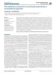
The integer program determines an assignment of vehicles to customers for each day. Once a solution is found for one day, the results are used to modify the rewards and costs for the next day. Unsatisfied demand at a customer in one day causes an increased revenue per unit delivered for that customer the next day. We used simulation to evaluate the performance of the policies for the larger instances. Starting at several initial states, both the policy produced by our algorithm and the policy of CBW were simulated. The integer program that forms the basis of the approach of CBW is given in Appendix A, and the problem instances used in both sets of experiments are given in Appendix B. The preliminary results are promising. Table 1 shows the maximum percentage differences over all states between the value functions V π1 , V π2 , V π3 , and V CBW , and the optimal value function V ∗ for problem instances given in Appendix B. The initial policy π1 is given by the optimal solution to the nonlinear knapsack problem (3), the second policy π2 is obtained after one iteration of our algorithm, and the third policy π3 is obtained after two iterations of our algorithm. V CBW is the value function of the method of Chien, Balakrishnan, and Wong. The value functions were computed using the Gauss-Seidel policy evaluation algorithm. The results show that for these instances, the policies produced by our method are very close to optimal and are consistently better than the policy of CBW. Figure 1 shows V ∗ , V π1 , V π2 , V π3 , and V CBW for instance 3. It is not only the maximum differences between V πi and V ∗ which are smaller than the maximum differences between V CBW and V ∗ , but V π1 , V π2 , and V π3 are consistently better than V CBW for all states.

Instance 1 2 3 4

Max percentage difference π1 π2 π3 πCBW 0.18% 0.002% 0.002% 0.54% 1.93% 0.22% 0.15% 5.22% 1.76% 0.009% 0.009% 10.02% 0.84% 0.15% 0.10% 16.36%

Table 1: Maximum percentage difference, maxx∈X {1 − V π (x)/V ∗ (x)}, between optimal value functions V ∗ and value functions V π1 , V π2 , V π3 , and V CBW , for problem instances given in Appendix B, obtained using GaussSeidel policy evaluation.

For larger instances, the Gauss-Seidel policy evaluation algorithm cannot be used to compute the value functions. The most important reason for this is that the number of states becomes too large, and the available computer memory is not sufficient to store the values of all the states. For larger instances, policies π3 and πCBW were evaluated by randomly choosing a number of initial states, and simulating the system under the different policies starting from the chosen initial states. Each replication produced a sample path over a relatively long but finite time horizon of 800 time periods. The length of the time horizon was chosen to bound the discounted truncation error to less than 0.01. Six sample paths were generated for each combination of policy and initial state, for each instance. The results are shown in Table 2. Also shown are the sample averages µ and sample standard deviations σ over the six sample paths, as well as intervals (µ − 2σ, µ + 2σ). As can be seen from the results, policy π3 consistently performed better than policy πCBW . The relative amounts by which policy π3

performed better than policy πCBW varied widely from instance to instance. We are investigating how these

10

Value *10-3

10.6

X1 = 10, X2 = 5 Optimal value Policy 1 Policy 2 Policy 3 CBW policy

10.2

9.8

9.4 0

1

2

3

4

5

6

7

8

9

10

Inventory at customer 3 (X  ) Figure 1: Optimal value function V ∗ , value functions V π1 , V π2 , V π3 , and V CBW , as a function of the inventory at customer 3, for instance 3 given in Appendix B. performance differences are related to the characteristics of the instances.

5

Future Work

The methods and results described in this paper represent only the initial stages of our research on the IRP. Much work remains to be done before some of the large IRPs encountered in practice can be solved. Even for the DDIRP several computational issues need to be addressed before larger instances can be solved. As the number of customers increases, the size of the action space A(x) increases rapidly. Thus methods should be developed

to determine the best action, or at least a good action, in A(x), without enumerating all actions in A(x). The effort required to compute the expected value in (4) also increases as the number of customers increases, and thus

there is a need for fast approximation methods to estimate the expected value. The convergence of the parameter estimates βs is slow, especially when using stochastic approximation. Improvements in convergence rates will also improve the usefulness of the proposed approach. An important extension of our work involves routing vehicles to more than one customer on a delivery tour. This version of the IRP is likely to be much harder than the DDIRP, since the optimization problem on the right hand side of (2) is much harder for the IRP than for the DDIRP. In the case of the IRP, this optimization problem involves solving both a vehicle routing problem, which is NP-hard, as well as determining the optimal quantities to be delivered to each customer on a delivery tour, which involves solving a nonlinear optimization problem with a nonunimodal objective function, as shown in Campbell et al. (1998).

11

Initial State 1,4,3,2,0 3,6,0,5,7 5,1,1,4,4 7,7,2,1,5

Initial State 6,2,3,7,3 0,10,0,10,4 2,5,0,10,9 10,6,8,6,0

Initial State 2,3,0,5,6,4 1,6,6,6,6,3 3,0,1,5,5,3 6,4,2,4,0,2

Initial State 3,4,0,7,8,6 1,8,8,8,8,4 4,0,1,6,6,4 7,5,2,5,0,3

Policy π3 πCBW π3 πCBW π3 πCBW π3 πCBW

Policy π3 πCBW π3 πCBW π3 πCBW π3 πCBW

Policy π3 πCBW π3 πCBW π3 πCBW π3 πCBW

Policy π3 πCBW π3 πCBW π3 πCBW π3 πCBW

81.47 78.80 81.09 78.61 81.77 78.84 79.82 78.55

Instance 5 Replicates for Values (∗10−3 ) 81.37 81.31 82.33 81.72 79.13 79.82 77.80 79.40 80.39 79.97 80.48 80.67 78.54 78.95 77.09 78.65 81.51 81.42 80.43 81.30 78.48 79.36 77.18 79.11 81.07 80.39 80.86 80.43 78.12 78.60 76.66 78.39

80.63 78.42 81.15 77.88 81.25 78.35 80.91 77.89

µ 81.47 78.89 80.63 78.29 81.28 78.55 80.58 78.03

σ 0.55 0.72 0.45 0.68 0.46 0.77 0.46 0.72

µ − 2σ 80.37 77.45 79.73 76.92 80.37 77.01 79.66 76.58

µ + 2σ 82.58 80.34 81.52 79.66 82.19 80.10 81.50 79.48

74.15 69.56 75.27 70.73 74.86 70.18 74.42 69.74

Instance 6 Replicates for Values (∗10−3 ) 75.67 74.87 76.14 77.10 69.20 68.82 70.02 69.92 75.70 75.15 76.43 77.28 69.79 69.52 70.53 71.36 74.17 74.16 75.33 76.97 69.09 69.30 70.25 70.05 73.62 73.54 74.86 75.94 69.68 68.82 69.79 69.45

74.84 68.55 75.19 68.58 74.62 68.03 74.16 67.57

µ 75.46 69.34 75.84 70.09 75.02 69.48 74.42 69.18

σ 1.06 0.59 0.86 0.99 1.05 0.86 0.89 0.86

µ − 2σ 73.34 68.16 74.12 68.10 72.91 67.76 72.64 67.45

µ + 2σ 77.59 70.53 77.55 72.07 77.13 71.21 76.21 70.90

52.18 41.51 51.70 41.32 52.03 41.94 52.07 40.52

Instance 7 Replicates for Values (∗10−3 ) 52.64 53.16 52.81 54.81 38.56 40.80 39.20 41.60 52.06 52.58 52.12 54.75 37.99 39.65 38.48 40.19 52.90 53.32 52.93 55.44 39.24 40.67 39.72 43.15 53.06 53.14 52.78 55.39 37.74 37.72 39.09 42.97

54.04 41.17 53.28 39.79 56.01 43.84 52.83 40.49

µ 53.27 40.48 52.75 39.57 53.77 41.43 53.21 39.76

σ 0.98 1.28 1.12 1.20 1.58 1.86 1.13 2.01

µ − 2σ 51.32 37.91 50.51 37.17 50.61 37.71 50.95 35.74

µ + 2σ 55.23 43.04 54.99 41.97 56.94 45.15 55.48 43.77

65.27 36.52 65.07 36.14 65.72 37.35 65.67 38.25

Instance 8 Replicates for Values (∗10−3 ) 64.83 65.65 64.97 64.61 35.77 34.33 40.11 37.24 64.33 65.44 64.76 64.49 35.59 32.41 39.72 35.90 65.25 65.81 65.43 65.17 36.05 33.10 40.94 39.24 64.93 66.04 65.36 64.87 36.12 34.48 40.41 38.02

64.02 35.34 65.14 37.98 65.36 35.21 64.76 40.22

µ 64.89 36.55 64.87 36.29 65.46 36.98 65.27 37.92

σ 0.56 2.01 0.42 2.46 0.26 2.83 0.51 2.31

µ − 2σ 63.77 32.54 64.03 31.36 64.94 31.33 64.26 33.30

µ + 2σ 66.01 40.57 65.71 41.22 65.97 42.64 66.28 42.54

Table 2: Values V π3 and V CBW for problem instances given in Appendix B, obtained using simulation.

12

Other issues that have to be addressed before IRPs can be solved in practice, include the estimation of the problem parameters. These include the rewards and costs, as well as the demand distributions. Estimating these parameters from noisy data lead to hard statistical and optimization problems. It is surprising how little work has been done in this area, since it is clear that the estimation of problem parameters from data is an essential activity for the formulation and solution of practical optimization problems.

References Anily, S. and Federgruen, A. 1990. One Warehouse Multiple Retailer Systems with Vehicle Routing Costs. Management Science, 36, 92—114. Anily, S. and Federgruen, A. 1993. Two-Echelon Distribution Systems with Vehicle Routing Costs and Central Inventories. Operations Research, 41, 37—47. Bard, J. F., Huang, L., P., J. and Dror, M. 1997. A Decomposition Approach to the Inventory Routing Problem with Satellite Facilities, Technical report, The University of Texas, Austin. Barnes-Schuster, D. and Bassok, Y. 1997. Direct Shipping and the Dynamic Single-depot/Multi-retailer Inventory System. European Journal of Operational Research, 101, 509—518. Bertsekas, D. P. and Tsitsiklis, J. N. 1996. Neuro-Dynamic Programming. Athena Scientific, Belmont, MA. Bramel, J. and Simchi-Levi, D. 1995. A Location Based Heuristic for General Routing Problems. Operations Research, 43, 649—660. Campbell, A. M., Clarke, L. W., Kleywegt, A. J. and Savelsbergh, M. W. P. 1998. The Inventory Routing Problem. In Fleet Management and Logistics. T. G. Crainic and G. Laporte (editors). Kluwer Academic Publishers, 95—113. Chan, L. M. A., Federgruen, A. and Simchi-Levi, D. 1998. Probabilistic Analyses and Practical Algorithms for Inventory-Routing Models. Operations Research, 46, 96—106. Chien, T. W., Balakrishnan, A. and Wong, R. T. 1989. An Integrated Inventory Allocation and Vehicle Routing Problem. Transportation Science, 23, 67—76. Dror, M. and Ball, M. 1987. Inventory/Routing: Reduction from an Annual to a Short-Period Problem. Naval Research Logistics, 34, 891—905. Dror, M., Ball, M. and Golden, B. 1985. A Computational Comparison of Algorithms for the Inventory Routing Problem. Annals of Operations Research, 4, 3—23. Federgruen, A. and Zipkin, P. 1984. A Combined Vehicle Routing and Inventory Allocation Problem. Operations Research, 32, 1019—1037. 13

Gallego, G. and Simchi-Levi, D. 1990. On the Effectiveness of Direct Shipping Strategy for the Onewarehouse Multi-retailer R-systems. Management Science, 36, 240—243. Golden, B. L., Assad, A. A. and Dahl, R. 1984. Analysis of a Large Scale Vehicle Routing Problem with an Inventory Component. Large Scale Systems, 7, 181—190. Haimovich, M. and Rinnooy Kan, A. H. G. 1985. Bounds and heuristics for capacitated routing problems. Mathematics of Operations Research, 10, 527—542. Jaillet, P., Huang, L., Bard, J. F. and Dror, M. 1997. A Rolling Horizon Framework for the Inventory Routing Problem, Technical report, The University of Texas at Austin, Austin, TX. Minkoff, A. S. 1993. A Markov Decision Model and Decomposition Heuristic for Dynamic Vehicle Dispatching. Operations Research, 41, 77—90. Nahmias, S. and Smith, S. A. 1994. Optimizing Inventory Levels in a Two-echelon Retailer System with Partial Lost Sales. Management Science, 40, 582—596. Trudeau, P. and Dror, M. 1992. Stochastic Inventory Routing: Route Design with Stockouts and Route Failures. Transportation Science, 26, 171—184. Van Roy, B., Bertsekas, D. P., Lee, Y. and Tsitsiklis, J. N. 1997. A Neuro-dynamic Programming Approach to Retailer Inventory Management, Technical report, Laboratory for Information and Decision Systems, Massachusetts Institute of Technology, Cambridge, MA.

14

Appendix A In this appendix, we present a slightly modified version of the method proposed by Chien, Balakrishnan and Wong (1989) (CBW), adapted for the DDIRP. At the start of each day, an integer program is solved to determine the vehicle assignments for that day. The parameters and variables of the integer program are given in the following table. n:

Number of customers

ri :

Revenue earned per unit delivered to customer i

ci :

Round-trip travel cost between depot and customer i

hi :

Holding cost per unit stored in inventory at customer i

pi :

Penalty per unit short at customer i

Ci :

Storage capacity of customer i

Xi :

Initial inventory at customer i

Di :

Estimate of the demand of customer i

m:

Number of vehicles

CV :

Vehicle capacity (for all vehicles)

dij :

Quantity delivered at customer i by vehicle j

yij :

1 if vehicle j is assigned to customer i, 0 otherwise

δi :

Lower bound on the final inventory at customer i

ηi :

Upper bound on the shortage at customer i

The integer program is given below.

Maximize

X i,j

ri dij −

X i,j

subject to

  X X 1X  ci yij − hi X i + dij + δi  − α pi ηi 2 i j i X dij ≤ Ci − Xi , ∀i

(8) (9)

j

dij − CV yij ≤ 0, X yij ≤ 1,

Xi + 

−  Xi +

X j

X j

∀i, j

(10)

∀j

(11)

dij − Di ≤ δi

∀i

(12)



∀i

(13)

i

dij − Di  ≤ ηi δi , ηi , dij ≥ 0 yij

binary

15

∀i, j ∀i, j

Constraints (9) ensure that the total amount of product delivered to a customer does not exceed the customer’s remaining capacity. Constraints (10) ensure that the amount of product delivered to a customer by a single vehicle is no more than the vehicle capacity. Constraints (11) ensure that a vehicle is assigned to at most one customer. Constraints (12) and (13) determine, for each customer, the final inventory or shortage at the end of the day. The P inventory at the end of the day is computed as max{0, Xi + j dij − Di }, where Di is taken to be the maximum P demand as suggested by CBW. Likewise, shortage is computed as max{0, −Xi − j dij + Di }. Note that by the

choice of Di , the holding costs are underestimated and the shortage costs are overestimated. This may result in a conservative low-risk policy.

The objective function consists of four parts: the revenue earned, the transportation cost, the inventory holding cost and the shortage cost. As proposed by CBW, the revenue earned per unit is given by ri + pi or ri depending on whether or not there was a shortage in the previous period. Their model has been modified slightly by incorporating a linear inventory holding cost given by half the sum of inventory after delivery and inventory at the end of the day, times the per unit holding cost. We have also assumed that shortages occur at the end of the day and are discounted at a rate α to the beginning of the day. Finally, it is assumed that the depot has an unlimited supply of the product.

16

Appendix B Instances for which the optimal value functions were computed. Instance 1 i

Ci

fi

ci

0

1

2

3

4

5

ri

pi

hi

1

5

0

0.2

0.2

0.2

0.2

0.2

50

80

50

15

2

5

0

0

0.5

0

0.4

0.1

20

100

50

15

3

5

0

0.4

0.1

0.2

0.1

0.2

20

80

50

15

n = 3, m = 2, CV = 5, α = 0.98 Instance 2 i

Ci

fi 0

1

2

3

4

5

6

7

8

9

10

ci

ri

pi

hi

1

10

0

0

0

0.5

0

0

0

0

0

0

0.5

120

80

40

10

2

10

0

0

0

0

0.5

0

0

0

0

0

0.5

80

80

50

5

3

10

0

0

0

0

0

0.5

0

0

0

0

0.5

120

100

50

5

ci

ri

pi

hi

n = 3, m = 2, CV = 7, α = 0.98 Instance 3 i

Ci

fi 0

1

2

3

4

5

6

7

8

9

10

1

10

0

0.1

0.1

0.1

0.1

0.1

0.1

0.1

0.1

0.1

0.1

120

80

50

5

2

10

0

0.1

0.1

0.1

0.1

0.1

0.1

0.1

0.1

0.1

0.1

120

80

50

5

3

10

0

0.1

0.1

0.1

0.1

0.1

0.1

0.1

0.1

0.1

0.1

120

80

50

5

hi

n = 3, m = 2, CV = 5, α = 0.98 Instance 4 i

Ci

fi 0

1

2

3

ci

ri

pi

4

1

4

0

0

0.5

0

0.5

100

80

50

5

2

4

0

0.25

0.5

0

0.25

120

80

50

10

3

4

0

0

0.5

0.25

0.25

120

80

50

5

4

4

0

0.5

0

0

0.5

100

80

60

4

n = 4, m = 3, CV = 3, α = 0.98

17

Instances evaluated with simulation. Instance 5 i

Ci

fi

ci

ri

pi

hi

0

1

2

3

4

5

6

7

8

1

8

0

0.4

0

0.1

0.1

0

0

0.2

0.2

40

100

50

2

2

8

0

0.1

0

0

0.4

0.4

0

0

0.1

30

120

50

3

3

8

0

0.125

0.125

0.125

0.125

0.125

0.125

0.125

0.125

45

80

70

5

4

8

0

0

0

0.3

0.3

0.3

0.1

5

8

0

0

0.1

0.2

0

0.2

0

0

0

50

80

40

4

0.2

0.3

40

80

30

3

n = 5, m = 3, CV = 8, α = 0.98 Instance 6 i

Ci

fi

ci

ri

pi

hi

0

1

2

3

4

5

6

7

8

9

10

1

10

0

0

0.2

0.3

0.4

0

0

0

0

0

0.1

100

180

40

15

2

10

0

0

0

0

0.4

0.4

0

0

0

0

0.2

100

80

50

5

3

10

0

0.4

0

0

0

0

0

0

4

10

0

0

0

0.3

0

0

0.3

0

0.5

0

0.1

120

40

30

15

0.3

0

0.1

140

80

25

5

5

10

0

0

0.1

0.2

0

0.2

0

0.2

0

0.2

0.1

120

120

50

15

n = 5, m = 3, CV = 8, α = 0.98 Instance 7 i

Ci

fi

ci

ri

pi

hi

0

1

2

3

4

5

6

1

6

0

0

0.5

0

0.5

0

0

60

80

40

5

2

6

0

0.1

0.1

0.3

0.3

0.1

0.1

50

80

50

8

3

6

0

0

0.5

0

4

6

0

0.1

0.1

0.3

0

0

0.5

40

80

30

5

0.3

0.1

0.1

40

80

20

5

5

6

0

0.5

0

0

0

0.5

0

50

80

50

15

6

6

0

0.1

0.1

0.3

0.3

0.1

0.1

60

80

70

5

ci

ri

pi

hi

5

n = 6, m = 4, CV = 5, α = 0.98 Instance 8 i

Ci

fi 0

1

2

3

4

5

6

7

8

0

0

0

0.5

100

80

40

1

8

0

0

0

0

0.5

2

8

0

0

0

0.5

0

0

0

0

0.5

100

80

50

5

3

8

0

0

0

0

0

0.5

0

0

0.5

120

80

30

15

4

8

0

0

0.5

0

0

0

0

0

0.5

120

80

20

5

5

8

0

0

0

0

0

0

0.5

0

0.5

120

80

50

15

6

8

0

0.5

0

0

0

0

0

0

0.5

120

80

70

5

n = 6, m = 5, CV = 6, α = 0.98

18