A finite temperature bridging domain method for MD-FE coupling .... In the fourth section we build a body with a free rough surface that is to be pressed against a.
A finite temperature bridging domain method for MD-FE coupling and application to a contact problem G. Anciauxa , S.B. Ramisettia , J.F. Molinaria,∗ a Ecole Polytechnique F´ ed´erale de Lausanne (EPFL) Facult´e ENAC-IIS, Laboratoire de Simulation en M´ecanique des Solides (http://lsms.epfl.ch/) CH-1015 Lausanne, Switzerland
Abstract A direct multiscale method coupling Molecular Dynamics to Finite Element simulations is introduced to study the contact area evolution of rough surfaces under normal loading. First, a description of the difficulties due to using the Bridging Domain Method at finite temperatures is discussed. This approach, which works well at low temperatures, is based on a projection, in an overlap region, of the atomic degrees of freedom on the coarser continuum description. It is shown that this leads to the emergence of a strong temperature gradient in the bridging zone. This has motivated the development of a simpler approach suitable for quasi-static contact problems conducted at constant but finite temperatures. This new approach is then applied to the normal loading of rough surfaces, in which the evolution of the real contact area with load is monitored. Surprisingly, the results show little influence of the contact area on temperature. However, the plastic events, in form of atomic reshuffling at the surface and dislocation activity, do clearly depend on temperature. The results show also a strong and temperature-dependent relaxation of the initial rough surfaces. This natural mechanism which alters atomic asperities brings to question the classical atomic description of roughness.
1. Introduction Contact between surfaces is essential in many natural processes and technological applications. Nonetheless, our understanding of contact mechanics and its important by-products which are friction and wear can arguably still be considered at its infancy. In contact problems, experimental, numerical or theoretical analysis is complicated by the wide range of phenomena that occurs concurrently at various scales. In the last decades, the advancement of Atomic Force Microscopy has generated a breadth of fundamental experiments that give us new hopes of understanding the origins of frictional forces. The push towards nanoscience and nanotechnologies, which emphasize surface mechanisms, has only exacerbated this strong interest. Not surprisingly, the number of both continuum and atomic scale studies of contact has seen a strong and recent increase. Perhaps one of the most fundamental sub problem of contact mechanics is that of two rough surfaces brought in normal loading. Traditional theories [1, 2, 3, 4] often assume that a stressed ∗ Corresponding
author Preprint submitted to Elsevier
March 11, 2014
solid with a rough surface responds elastically to external load. This leads to a linear dependence of the contact area with the applied pressure. The idea is that the applied stress allows more and more asperities to contact and thus sustain load. The fractal nature of surfaces is often a key point to exploit statistical properties on deforming asperities leading to the described linear behavior. Numerical studies [5, 6, 7, 8, 9] at both continuum and molecular levels showed that this trend is effective even when including plastic deformation. Finite element (FE) simulations [6] have also shown that the real contact is constituted of small clusters at which atomic interactions should dominate. This has motivated recent nanoscale contact simulations, in which the roughness dependency as well as the elastic-plastic contribution to the overall deformation were investigated [10, 11]. However, few studies have analyzed the influence of temperature on surface roughness and contact evolution. This is surprising since contact, especially during sliding motion, generates important temperature gradients due to plastic flow [12]. In this context surface topologies can be altered due to thermal expansion and the accompanying pressure confinement. Furthermore, heat generation and heat transfer through contacting asperities depend on the contacting profile [13]. The interdependency between surfaces and thermal conduction must be modelled correctly. Be it at the macroscale, for sliding or rolling contact, or at the nanoscale during nano-indentation or nanoscratching experiments, understanding temperature evolution and its influence on deformation mechanisms at interacting asperities is of crucial importance. In this work, we focus on the effect of temperature on normal contact. The study is conducted at the nanoscale using molecular dynamics as the principal model. This necessitates long simulation runs to let temperature equilibrate. In order to reduce the computational costs, we introduce a direct multiscale coupling between molecular dynamics and a finite element engine. One can distinguish two main coupling strategies. The first one merges interface atoms with boundary mesh nodes at a given interface in order to allow information passing [14, 15, 16]. Finite temperatures can be achieved by means of time averaging [17] or with an implicit modeling of thermal properties [18]. Nevertheless, the mesh constraint is very demanding. Indeed the mesh preparation needs the coupled nodes to match atomic sites. Furthermore, the mesh should then refine down to the atomic scale, which induces a large computational time. The other family includes a bridging zone [19, 20, 21, 22], which is a transition region where the atomic contribution is matched to continuum at a scale above. At low temperatures these methods were extensively studied to prevent spurious effects such as wave reflections [23]. To the best of our knowledge, finite temperature above hundreds of Kelvin were not considered in previous studies. In this paper, we will test the limitations of the Bridging Domain method, which applies a projection, before proposing a coupling strategy that can work well in threedimensional cases within a thermostated environment. In the next section, we present the details about the Molecular Dynamics (MD) model used to represent a perfect crystal copper. Thermal expansion is taken into account so that zero internal pressure is maintained. Then we present the coupling methodology, starting with a demonstration of the inherent limitations of projective methods, and our solution to palliate these difficulties. In the fourth section we build a body with a free rough surface that is to be pressed against a rigid flat plate. Then, we report our results regarding the influence of temperature on contact and pressure measurements, as well as on plastic activity at the contacting interface. Finally a discussion about the stability of the constructed surfaces is presented before concluding. 2
2. MD model The purpose of this section is to describe the MD simulation model. The simulation model uses a perfect FCC copper crystal. The Cartesian reference frame of axes is set along the lattice directions. The Embedded Atom Method (EAM) [24] is used to model the inter-atomic interactions. The basic equations of the EAM potential are described as: X 1X V(ri j ) + F(ρi ) 2 i, j,i i X ρi = φ(ri j )
Etot =
(2.1) (2.2)
j,i
where V is a pair potential, φ(r) is the electronic density contribution with respect to the distance r of a neighbor atom, ρi is the electronic density associated with atom i, ri is the position of atom i, ri j = r j − ri and ri j is the norm of the vector ri j . Then the force that is to be applied on a given atom k is: � � rik ∂Etot X � 0 = V (rik ) + F 0 (ρi ) + F 0 (ρk ) φ0 (rik ) (2.3) ∂rk rik i,k EAM potentials commonly define pair potential and electronic density by means of tabulated functions. In our simulations we used the functions developed by Mishin [25] that accounts well for the dislocations activation energies. Also a time step of 1 fs is used to integrate the governing equations of motion. One difficulty in finite temperature MD studies is that the crystal lattice parameter (referred to “a” later on) is temperature dependent. Thermal expansion must be taken into account in order to maintain constant pressure. We computed these lattice constants with a cubic simulation box made of 4000 copper atoms using NPT (constant number of atoms, pressure and temperature) ensemble. In these simulations the global domain size is allowed to vary in order to accommodate pressure and temperature effects. We introduced a zero pressure constraint and several temperatures were elected. Table 1 presents the obtained lattice constants as well as the thermal expansion coefficients. They match the values revealed by other studies [25]. The crystalline bodies used in our work were all built accounting for the thermal expansion. Temperature in Kelvin 100 200 300 400 500 600 700 800 900
Lattice constant in Å 3.620 3.625 3.631 3.637 3.643 3.650 3.657 3.664 3.671
Thermal expansion in 10−5 K −1 1.518 1.533 1.552 1.589 1.605 1.631 1.666 1.698 1.731
Table 1: Lattice constant and thermal expansion at different temperatures
3
3. Multiscale approach As mentioned earlier, we use a concurrent multiscale approach with atomic to continuum coupling to simulate the behavior of materials in contact. Full atomic details are retained in critical regions of the material where asperities are contacting (and exhibit a complex deformation behavior), while macro or continuum models are employed to describe deformation in regions more remote from the contact. Let us define ΩA and ΩFE the atomic domain and the continuum domain respectively. In ΩA the model introduced in the previous section is used. In ΩFE the well-known linear momentum balance expression for a continuum with no body force is used: ∇ · σ = ρ˙v
with
σ = C: �
(3.1)
where σ is the Cauchy stress tensor, ρ is the mass density, v is the velocity field and C is the elasticity tensor. For the copper material we use a constitutive anisotropic law that has the following elasticity tensor: 0 0 0 C11 C12 C12 C12 C11 C12 0 0 0 C C12 C11 0 0 0 (3.2) C = 12 0 0 C44 0 0 0 0 0 0 0 C44 0 0 0 0 0 0 C44 The elastic constants C11 , C12 and C44 were computed in [26] at various temperatures and are recalled in table 2. Temperature in Kelvin 100 200 300 400 500 600 700 800 900 1000
C11 171.0 163.2 160.2 152.1 143.2 140.4 131.5 123.8 111.5 106.1
C12 119.6 114.8 112.3 109.2 102.2 99.8 96.6 94.4 84.2 81.9
C44 78.5 75.4 72.2 69.9 66.4 61.6 58.8 54.8 54.1 51.1
Table 2: Elastic constants in GPa at different temperatures from [26]
In the Bridging Domain method [19, 20], FE and MD models are used to represent continuum and fine (atomic) scales respectively while a transition region allows the proper handling of wave reflections at low temperature [23]. But, to the best of our knowledge this method was never tested in a true finite temperature situation. In the following subsection we first recall the coupling details before presenting the problems occurring for finite temperatures. Ultimately we introduce a correction that prevents problems related to thermal fields. 4
3.1. Bridging Domain method We refer to the coupling method introduced by Belytschko and Xiao [19], which couples continuum models with molecular models using an overlapping region ΩR , in which both the continuum and molecular domains coexist. A global Hamiltonian is taken as the sum of the weighted Hamiltonians of both the molecular and continuum parts. The global multiscale Hamiltonian is simply given as H = E A + EC (3.3) where E A and E C are the atomic and continuum Hamiltonian contributions, expressed as P P E A = qi ∈ΩA \ΩR Ei (qΩA ) + qi ∈ΩR (1 − α(Xi ))Ei (qΩR ) (3.4) EC =
P
e∈ΩFE \ΩR
Ee (uΩFE ) +
P
α(X)δEe (uΩR )dX e
R e∈ΩR
with Ei the energy fraction for atom i, Xi its initial position, Ee the energy fraction for element e, δEe its potential energy density and α stands for an arbitrary weighting function. Here the notation q represents the vector of atomic positions while u represents the nodal displacements vector. In addition qΩA , qΩR , uΩFE and uΩR refer to spatial zones: they are used to indicate that a subset of the degrees of freedom (DOFs) is considered. The two models are coupled in the bridging sub domain by constraining the DOFs in order to enforce the displacement continuity using a Lagrangian constraint formulation. The constraints in the bridging sub domain (ΩR ) hold on velocities and are expressed as: X ϕ J (Xi )u˙ J − d˙ i = 0 (3.5) ∀i ∈ ΩR gi = J
where ϕ J denotes the shape function associated to node J. For notation purposes, we consider indexes in upper case and in lower case to refer to finite-element quantities and atomic quantities respectively. If there are L atoms in the coupling zone ΩR then L constraints are considered. The governing equations for the coupled multiscale domain are then formulated using the Lagrangian multiplier method. The Lagrange multipliers Λ = (λi )i=1..L are obtained by solving the linear system of equations HΛ = g? (3.6) with g? the value of the constraint vector before correction and H is the L × L constraint matrix defined as X ˆ J−1 − m Hi j = ϕ J (Xi )ϕ J (X j ) M ˆ −1 (3.7) i δi j J
ˆ I = α(XI )MI and m where M ˆ i = (1 − α(Xi ))mi , considering that MI is the lumped mass on node I and mi is the mass of atom i. Finally, considering the modified forces fˆi and fˆI (due to the weighted Hamiltonian), the discrete governing equations within the two models are expressed as follows: ( L ˆ I u¨ I = fˆI − Pk=1 M λk ϕI (Xk ) (3.8) ˆ ¨ m ˆ i di = fi − λi for which the integration in time is performed using the SHAKE algorithm [27]. Details of the derivation of the above equations are presented in [19, 20, 23]. We insist again on the fact that both FE and MD DOFs of the overlapping area are modified by the application of the constraint. This brings consequences in the finite temperature regime as discussed in the following subsection. 5
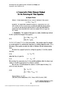
Figure 1: Model used to test the Bridging Domain. The coupling area is presented in red, while the white upper zone is constituted of atoms and the white bottom zone is continuum only. The top blue layer is a region of fixed atoms that provides a boundary condition to the atomic model.
3.2. Finite Temperature with the Bridging Domain Since we wish to investigate the influence of temperature on contact evolution, we seek to apply a finite temperature throughout the substrate body. To that purpose we use a thermostat in the atomic zone. The coupling scheme will change the temperature field as we demonstrate below. In essence the Bridging Domain can be considered as a projection that pushes gradually the atomic DOFs to the interpolated continuum fields. These are obviously smoother than the noisy atomic description of velocities. While we try to maintain constant temperature, the coupling scheme has a cooling effect on the coupled atoms. Let us define the simplest patch test to evaluate the capacity of a coupling method at finite temperatures. This test considers a piece of material at uniform temperature and zero pressure. In such conditions, mechanical and thermodynamic equilibrium is initially set. Thus, for a robust coupling method, temperature should remain constant. Let us introduce the geometry defined in figure 1. The top part (ΩA ) is modelled with MD while the bottom part (ΩFE ) is driven by finite elements. The overlapping zone follows the Bridging Domain strategy. For the boundary conditions we maintain fixed the top layer of atoms (presented in blue), as well as the bottom free surface of the mesh. In the other two directions periodicity is imposed. The temperature is maintained to a constant value by means of a Berendsen [28] thermostat which includes a viscous force that is applied to thermostated atoms. This leads to a rescaling of atomic velocities by a parameter α following: r � M t � T0 α= 1+ −1 (3.9) τ T where ∆t is the time step used, τ is a time parameter that sets the strength of the coupling with the heat bath, T 0 is the heat bath temperature and T is the actual temperature of the domain. Such a thermostat is applied in the atomic zone ΩA \ ΩR which excludes coupling and finite element 6
(a)
(b)
Figure 2: Temperature profile along the vertical direction (a). The decay of temperature is particularly evident. The temperatures were extracted along a vertical line as presented on the left image of (b). The kinetic energy removal happens very quickly. At time t = 0 no projection is applied, and already at time t = 1ps the projection dropped almost all temperature in the coupling region as seen in (b). The temperature profiles issued from a full molecular dynamics simulation is presented for comparison purposes. The non-physical temperature gradient created is due to the projective nature of the Bridging Domain method. An important point to note is the impact on the non-coupled zone of the temperature profile which implies a strong modification of the dynamics in ΩA .
zones. Therefore, atoms in the coupling zone (colored in red) are driven by their proper dynamics and the coupling corrections. The dynamic evolution of the model was computed with no load. Temperatures of 100, 200 and 300 Kelvins were considered. After a few time steps, the coupling has effectively changed the temperature profile as can be seen in figure 2. Also, the temperature profiles that are obtained by using only molecular dynamics with no coupling were extracted and are presented in this figure. Again, the temperature through the bridging zone cannot be constant since the coupling algorithm projects the noisy velocities of single atoms to the much smoother continuum velocity field. The difference in scale from atomic to the defined mesh leads to an impossibility of representing very high frequencies. Therefore, as heat within MD is represented by atomic lattice vibrations, the projection results in a temperature drop in the bridging zone. We note here that this has also an effect on the atoms in ΩA since the Berendsen thermostat is maintained globally. This explains why, in a region, the temperature is above the thermostated temperature (see figure 2). Clearly, our coupling (and projection) strategy is not suitable for a finite temperature problem since it impacts temperature also in the uncoupled zone. This temperature change induces yet another side effect. Indeed, the introductory part presented that the volume of the copper crystal was set accordingly to maintain zero pressure and constant temperature. Since the projection modifies the kinetic energy of the coupled atoms, these want to shrink their attributed volume in order to go back to ground state. Ultimately, this temperature decrease manifests mechanically as an internal spurious displacement along the negative temperature gradient in the coupled area. Arguably, the observed displacements are small (∼ 0.8 Å at 500K) and may be considered as a small side effect compared to the temperature gradient. Despite our best efforts, we could not find an easy scheme to compensate for this temperature gradient and the shrinkage sustained by the coupled atoms. Since the coupling damps quite strongly kinetic energy it makes any thermostat in ΩR unusable (and unstable) to fix this temperature decrease. Concerning the internal displacement, the use of a force in a single direction 7
(a)
(b)
Figure 3: On subfigure (a) we present the proposed coupled domain used with finite temperature. Besides the atomic zone (ΩA ) and the continuum zone (ΩFE ), two zones are defined where coupling is done separately. In Ω1 mesh nodes are constrained to atomic mean displacement and in Ω2 atomic displacements are interpolated from the mesh to provide a moving boundary condition to ΩA . Subfigure (b) shows the temperature profiles obtained with the method proposed in section 3.3.
cannot compensate a volumetric change. A patch to these problems would require changing the inter-atomic potential, which is technically complex. Instead, we changed the coupling method, so that no temperature cooling would take place. This is the purpose of the next section. 3.3. Multiscale coupling at finite temperature In order to achieve a reasonable coupling that does not lead to an artificial cooling of the system, the previously presented set of equations must be changed. Indeed, we need to remove any projection that modifies the atomic field and thus would damp a part of the kinetic energy. We will separate the coupling in two zones Ω1 and Ω2 as depicted in figure 3. In the first one the atomic DOFs will not be modified whereas the continuum DOFs will be constrained to match the atomic solution. Thus the kinetic energy of these atoms is left untouched preventing the previously mentioned side effects and providing a mechanism for passing information from MD to FE. In Ω2 , the reverse operation is performed by constraining atoms to the continuum fields by means of a simple interpolation. One inconvenient is that no wave reflection treatment is introduced here but The following procedure is thought only for constant finite temperatures. In Ω1 we constrain the mesh nodes to atomic displacements. Since mesh nodes in the bridging zone are now fictive and purely driven from MD, let us consider the following constraints: gi =
X
ϕ J (Xi )uJ − di
(3.10)
J
where mesh nodes are to be corrected and the atomic velocities and positions are not modified. 8
In Ω1 the governing equation for continuum DOFs is: MI u¨ I = fI −
L X
λk ϕI (Xk )
(3.11)
k=1
The SHAKE [27] integration scheme provides: n+1/2 ∆t n ∆t PL u˙ I = u˙ nI + 2M fI − 2M k=1 λk ϕI (Xk ) I I n+1/2 n+1 un+1 ˙ = u + ∆t u I I I evaluation o f fIn+1 u˙ n+1 = u˙ n+1/2 + ∆t f n+1 I I 2MI I
(3.12)
with the requirement that the constraint function should be respected, we combine 3.10 and 3.12 to obtain: L X X X ϕ J (Xi )ϕI (Xk ) ? (3.13) ϕ J (Xi )uJ − di = λk MJ J J k=1 ∆t n Where u?n+1 = unI + u˙ nI + 2M f . It also means that ? superscript denotes displacement values J I I before the application of the constraint. Thus a new constraint matrix H is defined so that: 2
Hi j =
X ϕ J (Xi )ϕI (Xj ) J
MJ
(3.14)
It leads to a comparable linear system Hλ = g? to solve in order to compute the multipliers. Once the Lagrange multipliers are obtained, we can constrain the nodal displacements to a coherent state with the atomic displacements. However the formulation also needs a correction of the velocities. Finally, the following algorithm is to be used: ∆t n f (1) u˙ ?I = u˙ nI + 2M I I ? n (2) uI = uI + ∆tu˙ ?I P (3) g?i = J ϕ J (Xi )u?J − dn+1 i (4) λi = Hik−1 g?i ∆t PL (5) u˙ n+1/2 = u˙ ?I − 2M k=1 λk ϕI (Xk ) I I 2 PL ∆t n+1 ? (6) uI = uI − 2MI k=1 λk ϕI (Xk ) (7) evaluation o f fIn+1 ∆t n+1 f (8) u˙ n+1 = u˙ n+1/2 + 2M I I I I (9) Go back to (1)
(3.15)
Clearly this creates a one way coupling process from MD to FE. The reverse exchange of information is then processed in Ω2 by providing a moving boundary condition to the atomic model. The temperature of boundary atoms is now related to the vibration modes of the finite element part. Since the velocity of mesh nodes are smaller, because of the change of scale, the imposed velocity onto the atoms is almost zero. Nevertheless no thermal energy flux is occurring in that area, as revealed in figure 3 which shows a constant temperature profile. This method was used with the previously defined patch test with success. We also loaded the top surface and verified that the final static state was coherent with continuum theory. Nevertheless this method can probably not be applicable in NVE (number of particles, volume and energy 9
remain constant) ensemble at very low temperatures since the amount of kinetic energy trapped by reflections at the interface would modify the dynamics of the MD region. But projection methods are not applicable here as well due to thermal expansion. Our proposed coupling scheme shares common features with seamless methods [17]. One may therefore question the utility of bridging zone at all when no wave reflection treatment is performed. Indeed, CADD method has been used at finite temperature with nodal time averaging to transfer mechanical fields at thermodynamic equilibrium [17]. Here, the same goal is achieved, but the overlap region opens perspectives for computation of local temperatures and heat fluxes which seems very difficult in the context of an edge-to-edge coupling formulation. Another advantage of overlapping methods stands in the reduction of the number of degree of freedom since, in opposition to seamless methods, the finite element mesh does not need to be refined down to the atomic scale. Our method is thought to be a starting point for an energy balance equation that would lead to proper treatment of energy fluxes.
4. Results This section presents the obtained results concerning a normal loading of rough (self-affine fractal) surfaces. Our setting considers the loading of a flat surface (moving downwards) onto a deformable rough surface which is maintained at a desired temperature. To construct such a surface we first consider a pristine piece of crystalline copper in which we cut a fractal surface. The description of the fractal surface is given by a Voss [29, 30] algorithm. Also we took into account the thermal expansion described in section 2. We prepared two 3D geometries with different surface roughness. As illustrated in figure 4, one surface was parameterized to a Hurst exponent H = 0.7 and root mean square of heights ∆rms = 10a while a flatter one was set to have H = 0.8 and ∆rms = 5a. In both cases, the section is L2 with L = 32a, which is small enough to allow fast computations on a parallel computing machine while having around 100 000 atoms in the atomic zone. The deepness of the atomic domain is also taken as 32a but since some layers where removed at the free surface the exact global height is effectively a little reduced. Nevertheless, the coupling allows to have an additional elastic zone of 64a being 128 additional atomic layers. The mesh is made of 10 × 10 × 20 elements. While the inter-atomic potential used for the substrate is the EAM described previously, the interactions between atoms from the√rigid plate and substrate have been modified: a Lennard Jones potential with a cutoff radius of a 2/2 (first neighbors distance) is used in order to discard the adhesive forces (removing the adhesive forces when using EAM is a complicated task since the electronic contribution is not a pair-wise term). Before loading the rigid plane the substrate is allowed to equilibrate to a required temperature, which modifies the surface as will be presented later. Again, the constant temperature was constrained using a Berendsen thermostat [28]. The thermostat was applied on the molecular part since the continuum zone only handles mechanics. After equilibration, we allow the top flat rigid surface to descend downwards and create contact in reaction to an applied initial pressure of 0.1 GPa. The pressure is regularly incremented by 0.1 GPa every 10ps. Thus the loaded surface has 10ps to equilibrate, which establishes a quasi-static loading of our substrate. The simulation was run on a parallel cluster, with one processor dedicated to finite element elasticity, while 32 processors were occupied in the time integration of molecular dynamics. 10
Figure 4: The surface profiles obtained with a Voss [29, 30] algorithm are presented. Underneath, the substrate is composed of copper atoms. The flat body above the substrates is the rigid surface to be pressed against the rough surfaces. The left surface is flatter than the one on the right.
We used LAMMPS1 for molecular dynamics and a in-house code for finite elements, while LibMultiScale [31] was carrying the coupling process. 4.1. Measurement method for contact area and load As our objective is to follow the evolution of the contact area with load, it is necessary to monitor precisely the applied pressure. We impose a constant pressure on the rigid body following the same strategy depicted in [32]. We set the center of mass of the top body to move according to a unique force. This force is computed with: X F= f at − P · L2 (4.1) at
where P is the desired pressure, and f at is the initial per atom force issued from standard molecular dynamics. We then “distribute” such a force over all the atoms so that the resulting atomic acceleration becomes uniform and follows: P at f − P · L2 ∀i ∈ Ωrigid , ai = at (4.2) mr with Ωrigid the domain of the rigid plate and mr the mass assigned to each atoms in Ωrigid . We reduced arbitrarily the mass of these atoms so that the contacting force is transmitted with reduced inertial effects. We used mr = �mcu with mcu being the mass of a single copper atom. Having �