A Framework for Interpolating the Population Surface at the Residential-Housing-Unit Level Zhixiao Xie1 Geosciences Department, Florida Atlantic University, 77 Glades Road, Boca Raton, Florida 33431
Abstract: Population surface information is essential for a broad array of geographical studies. Many areal interpolation methods have been developed for creating population surface data from decennial census data. This paper describes a new framework to interpolate population to the lowest spatial level, i.e., housing units, based on high-resolution geospatial imagery. The framework is fundamentally a dasymetric mapping process, comprising: (1) determination of the basic dasymetric unit; (2) extracting the basic units; and (3) allocating population counts to each unit. An example was carried out to illustrate the promises and challenges of implementing such a framework using DOQQ, LIDAR, and parcel data.
INTRODUCTION The spatial distribution of a population or population surface is an essential variable for a broad array of geographical studies in which the spatio-temporal coupling of population and other physical and socio-economic processes is of concern—e.g., environmental health, crime mapping, environmental (in)equity and more. In the United States, the decennial census data set provided by the U.S. Census Bureau is one publicly available, commonly used population data set. Due to privacy and reliability concerns, population data from the decennial census are usually reported at various levels of areal units with roughly similar counts of population—e.g., census tract, block group, blocks. The use of the census areal units for population surface analysis introduces a variety of issues. Partitioned in an arbitrary manner, these areal units vary widely in shape, size, and population totals (Dorling 1993). An obvious application issue is the possible incompatibility of areal units when analysis needs to incorporate other social-economic and environmental datasets; i.e., the spatial areal units of different data are often not the same, because these data may come from different sources, be collected at different times, and for different applications (Xie, 1995). Another relevant issue is the modifiable areal unit problem (MAUP) (Openshaw, 1983), referring to the fact that the results of spatial data analysis may depend heavily on where the areal boundaries are laid and the scale at which data are aggregated. 1Email:
[email protected]
1 GIScience & Remote Sensing, 2006, 43, No. 3, p. 1–19. Copyright © 2006 by V. H. Winston & Son, Inc. All rights reserved.
2
ZHIXIAO XIE
The areal unit incompatibility issue can be solved through areal interpolation (Goodchild and Lam, 1980), a process used to transform data from one system of areal units (source zones) to another (target reporting zones) (Xie, 1995). Over the past two decades, many different methods have been developed for areal interpolation in a GIS environment (e.g., Goodchild and Lam, 1980; Xie, 1995; Martin et al., 2000; Mennis, 2003; Reibel and Bufalino, 2005). For the MAUP problem, one key aspect is the scale of analysis. Some argue that a spatial analysis should be conducted at a scale level of areal units “appropriate” for the issue (Anderton et al., 1994). Others believe the analysis may only reveal meaningful and reliable results by examining the phenomena at multiple scales (Sui, 1999; Mennis, 2002), and that a statistical surface of population (in raster format) may facilitate such multiscale analysis (Mennis, 2002). The present study establishes a novel framework for interpolating Census population to the lowest level, i.e., the residential housing unit, using high–spatial resolution geospatial data. To the author’s knowledge, no previous research has been conducted to reveal population distribution at such a fine scale. The following sections describe relevant literature on areal interpolation, a new interpolation framework, implementation, and conclusions. RELEVANT LITERATURE ON AREAL INTERPOLATION This section does not intend to give a complete review of all literature on areal interpolation. Instead, typical approaches are introduced that led to the development of the new framework. Interested readers can refer to more complete discussion of the subject (e.g., Goodchild et al., 1993; Xie, 1995; Either and Brewer, 2001). Areal interpolation belongs to a broad category of spatial transformations named basis change (Goodchild et al., 1993), defined as the transfer of attributes from one set of objects to another. In areal interpolation, the spatial basis (or kind of objects) is area or polygon. To transfer attributes from one area basis to another, interpolation often resorts to the spatial relationship of the two sets of area basis (polygon objects), and/or ancillary attribute information. In the following sections, I review some major information used for areal interpolation and interpolation methods. Areal Interpolation Based on Spatial Relationships One type of areal interpolation is based solely on the spatial relationship between the source (reporting) zones and target zones. The representative approaches include area-based (areal weighting), and distance-based (centroid-based model) approaches. Areal weighting is used in cases where one can reasonably assume that the variation of population density (or other variables) within each source zone is homogeneous (Goodchild et al., 1993) or the population is evenly distributed within each source zone (Xie, 1995). If this assumption holds true, the derivation of the target-zone population is straightforward. The interpolation starts with an overlay process to create a set of intersection polygons from the source zones and target zones. Assume that a target zone t intersects with total m source zones. Denote the population in source zone s by pops, the
INTERPOLATING THE POPULATION SURFACE
3
area of the source zone s by areas (s = 1 ... m), the area of overlap between s and t by areast. The target-zone population popt can be estimated from pop t =
m
∑
s=1
pop s ( area st ⁄ area s )
(1)
If Equation (1) is used for population count, it has to be modified to interpolate population density. Nevertheless, one major flaw for areal weighting areal interpolation is that the assumption of homogeneous density may not hold for most socioeconomic variables within reporting source zones (Goodchild et al., 1993). A typical distance-based model is the centroid-based model originally developed by Martin (1989) and Bracken and Martin (1989). In this model, a populationweighted centroid location is known for each irregular source reporting areal unit. It is assumed that the centroid is the summary point for a small area around the point and that the population count for the areal unit follows an unknown kernel distribution, whose width may be adjusted based on distances between local centriods. The model intends to interpolate a raster-based surface representation of population count. In the interpolation, each cell may receive population redistribution from many centroids or none at all, and the redistribution amount may be weighted by a distance decay function (Martin et al., 2000). This approach was used in estimating population surfaces in the United Kingdom using a 250 m kernel width (Martin et al., 2000). However, guessing the “right” kernel function and the kernel width was not an easy task. Areal Interpolation Incorporating Ancillary Information The use of ancillary information is based on the assumption that population density is correlated with other socio-economic variables and that the spatial distribution of these variables can help interpolate population distribution. It is generally conducted via dasymetric mapping, the process to produce maps to depict quantitative areal data using boundaries that divide the mapped area into zones of relative homogeneity to best portray the underlying statistical surface (Either and Brewer, 2001). Based on Either and Brewer (2001), areal interpolation involving ancillary information is a dasymetric mapping process plus a final step to re-aggregate to the target reporting zone units. The most commonly chosen ancillary information is land use and land cover classes, and one earlier example goes back to a widely cited study by Wright (1936) in Cape Cod. To estimate population density variation under each township with a known average density, Wright (1936) first marked off “uninhabitated” areas based on USGS topographic maps supplemented by personal recollections, in a “rough-andready manner,” and population was only re-assigned to remaining “inhabitated” areas. The “inhabitated” areas were further divided into areas of different densities based on settlement patterns using two constraints: (1) the known average density of the township as a whole was maintained when setting the values of different densities within a township; and (2) the same density types across townships were adjusted to similar values. This concept was followed and implemented by many studies with various
4
ZHIXIAO XIE
refinements and was later referred to as the limiting variable method (Either and Brewer, 2001). A closely related areal interpolation type is called the three-class method (Either and Brewer, 2001), a method based on assigning varied percentages of total population of a county to only three different land use classes: urban, agricultural/woodland, and forested. The percentages were chosen subjectively, 70% to urban, 20% to agricultural/woodland, and 10% to forested (Either and Brewer, 2001). Besides the subjective percentage designation, this method did not consider different sizes of the three land use types within a county. In a recent study in Pennsylvania, Mennis (2003) developed a method to redistribute the population of each block group into grid cells (100 × 100 m) to create a population surface using the three-class method. However, Mennis (2003) further considered the relative differences of population densities among three urbanization classes and the area percentage of three classes within each block group. In addition, area percentage was derived empirically by sampling and analyzing block groups within each urbanization class. Another set of studies built upon quantitative equations linking population density with land use types based on empirical investigation (e.g., Langford et al., 1991; Martin et al., 2000). These studies first derived land use information from satellite imagery through image classification. Regression models were then established to estimate population densities for various land use categories. The original implementation (Langford et al., 1991) could not guarantee to preserve the population count at the original source zone level, and was refined in later studies to “preserve volume” (Martin et al. 2000). In their case study in Northern Ireland (Martin et al., 2000), an original source zone (ED—enumeration district) was classified into two groups of cells of either “built” or “unbuilt,” based on Landsat TM imagery re-sampled to 25 m spatial resolution. Then a global regression model was built with ED population as the dependent variable, and the number of built and unbuilt cells in the ED as independent variables. The model was finally used to estimate the output population surface with each cell of 200 × 200 m. Network-Based Areal Interpolation Network-based methods incorporate a special type of ancillary information: street segments (Xie, 1995). These methods are based on the observation that the houses in which people are sheltered are often sited along streets or roads, and hence the street segments or network should provide important supplementary information for population distribution in an area. In the first implementation, the network length method (Xie, 1995), an even distribution of population was assumed along the streets in each source zone and the length of the street segments plays a role similar to area in the areal weighting approach for population re-distribution into target zones. The second implementation, network hierarchical weighting method (Xie, 1995), considered the differences of residential densities or population concentrations along different categories of roads and assigned different weights to account for the differences. While improved over the network length method, the network hierarchical method was limited by the challenge to assign meaningful weights to each street class. The third method was called the network housing-bearing method (Xie, 1995). It was based on two key assumptions: (1) population within each source zone was
INTERPOLATING THE POPULATION SURFACE
5
evenly distributed in housing units—i.e., each house unit was assumed to contain the average number of persons for that source zone; and (2) the number of houses along each street segment can be derived by the address ranges along both sides of the street segment and the houses are distributed evenly along both sides. Therefore each unit length of each street segment was in fact associated with a certain number of houses, and also a population count. The population for each target zone was the sum of population linked to each street segment within the target zone. The concept for this method is attractive, although it can be improved dramatically by taking into consideration recently available geospatial information, as described in the new framework in the next section. A NEW FRAMEWORK FOR POPULATION INTERPOLATION AT THE RESIDENCE HOUSING UNIT LEVEL General Conceptual Framework This section describes a new framework to interpolate population at the residential housing unit level. Several issues essential for the interpolation framework will be discussed, including determination of the basic dasymetric units, defining spatial locations for these units, and allocating the population count to each unit. Determination of the Basic Dasymetric Unit. The interpolation framework is based on dasymetric mapping and requires that the mapped area be subdivided into basic dasymetric units of relative homogeneity to portray the underlying statistical surface. Obviously, it is important to first determine what should be the appropriate basic unit, particularly if it is based on U.S. decennial census data, which is the data source of paramount importance in the United States. Population is discrete in nature and the location of each individual is fundamentally uncertain, partly due to migration and diurnal movement (Goodchild et al., 1993). Collectively, population distribution is dynamic and a population surface only captures the picture for a specific time or time period. Indeed, a census decennial data set is a snapshot of the situation when the survey is conducted. Although considerable information is collected from individual persons and later summarized to either the block or block-group level for privacy and reliability consideration, the housing unit address is the smallest exact spatial information for all the members in a household. Therefore census population data are really about residential population, and the finest meaningful basic spatial unit is the housing unit. It is not possible to produce improved location information for residential population at a resolution finer than the housing unit, if the analysis is based on decennial census data, because the internal structure of a housing unit as well as the resident information will generally not be available (if we had the latter information, areal interpolation would not needed at all). Moreover, further subdividing a housing unit is not necessary for describing where a person resides for most geographical applications. The raster data model–based population surface representation and interpolation implicitly use a raster cell as the basic unit, with the primary purpose to ameliorate the MAUP and facilitate re-aggregating the population to into target areal units. It can be argued that the use of the residential housing unit as the basic unit is also well suited for re-aggregation, but with the advantage of treating the housing unit as an indivisible
6
ZHIXIAO XIE
whole. On the one hand, people reside in an actual housing unit instead of cells. Therefore, a housing unit (object)–based approach is closer to everyday perception and is a more appropriate representation of reality. Conversely, the use of raster cells will segment an integrative whole of a housing unit into parts. Finally, the housing unit based representation can still be implemented using a raster data model if necessary. Defining Spatial Locations for the Housing Units. The next important issue is to delineate the exact shape of the housing units and to determine their spatial location, so that the population count can be accurately assigned to them. Remotely sensed data are usually an essential part of such a task for up-to-date and large-area coverage. However, remotely sensed data at a coarse spatial resolution were never intended for and incapable of accurately distinguishing individual residential buildings and housing units. Coarse resolution data are better suited to producing more generic land use and land cover types. Similarly, the census TIGER/DIME street data, although useful for certain applications, can only be used to approximate a geocode residential address at a point along a linear street segment. Neither the location nor the shape of the housing unit can be accurately determined. Recently available high spatial resolution remotely sensed data, including highresolution satellite imagery, digital orthophoto imagery, and LIDAR data, supply partial solutions with the spatial and spectral detail they convey. However, remotely sensed data processing itself is not sufficient in most cases. In general, remotely sensed data can be used to capture the structural information of geographical entities, but can rarely be used to extract sufficient functional information associated with the manmade entities. Specifically no known algorithms can automatically extract residential buildings and housing units only (as opposed to commercial, public, or industrial buildings) from a complex geographical context, although buildings can be relatively reliably outlined. In this new framework, the author proposes to incorporate the rich information contained within a GIS-based land information system designed primarily for tax assessment, planning, zoning, etc. at the local level. This information will be essential for differentiating residential buildings from other buildings, and used to delineate the housing units. Allocating Population Count Data to Housing Units. In the network housingbearing model (Xie, 1995), each house number was given the average population for the source zone where the house was sited. Although it is reasonable to use average population count, that model did not consider the differences among varied categories of residential buildings. One house number in a TIGER/DIME street segment may be linked to multiple housing units, especially if a building contains multiple housing units as in a high-rise apartment complex. The allocation of population simply based on house numbers in such cases may severely distort the spatial distribution of population. There may be different solutions to this issue, although the basic principle is that we should take into account the different residential building types and process them accordingly. The case study will demonstrate one solution based on parcel data and tax roll information. The above discussion has outlined in concept terms the new framework for interpolating residential population at the residential housing unit level. The implementation details have been omitted, because it is believed that the framework may be implemented differently depending on the data and algorithms selected. The following
INTERPOLATING THE POPULATION SURFACE
7
Fig. 1. The study area in Boca Raton, Florida.
section describes one example of implementing the new framework as well as the possible issues. An Implementation Illustration Study Area and Data. This implementation illustration is based on data in Boca Ration, Florida (Fig. 1). The city encompasses 29.6 square miles (18,572 acres), and was incorporated in 1925 at the height of the Florida land boom. During another great land boom in 1960s, the town’s population grew to almost 30,000 residents, and by 2004, the city had 83,960 residents. Boca Raton is known internationally as an originator of comprehensive zoning. Within its city limits, diverse land uses exist. Since the city boundary does not coincide perfectly with census unit boundary, the study area actually includes parts from two other neighboring localities. The data used in this study include: Census Bureau decennial data, USGS Digital Orthophoto Quarter Quads (DOQQ), LIDAR data, and digital parcel data (Fig. 2). Population data were obtained from the 2000 Census Bureau decennial population data set at the block group level. DOQQ data represent large-scale ortho-rectified high spatial resolution aerial photography. The data were obtained on January 20, 1999 and digitized to a spatial resolution of 1 × 1 m. LIDAR is an active remote sensing tool used to measure the elevations of ground targets. It is based on the laser pulse travel time from the transmitter to the target and back to the receiver (Jensen, 2000). LIDAR data were collected between December 1999 and March 2002 using an Optech ALTM 1233 LIDAR mapping system and were processed by Florida International University International Hurricane Research Center (IHRC). Two types of raster surface DEM data were produced: a top-surface data set and bare-earth data set. Each data set was output to a 5 × 5 ft. raster grid with a vertical root mean squared error (RMSE) of 0.41 feet (12 cm) [http://gislab.fiu.edu/ ihrc/, last accessed January 10, 2006]. The top surface DEM represented the elevation of the top surface of the study area, while the bare-earth data set represented the elevation after the buildings and vegetation were removed. Both DEM data sets were
Fig. 2. Data for the study area. A. DOQQs. B. Bare-earth DEM. C. Top_surface DEM. D. Parcels. E. Census block groups.
INTERPOLATING THE POPULATION SURFACE
9
re-sampled to 1 × m spatial resolution so that the data could be easily related to the DOQQ. By definition, parcel information is all the documents, maps, and information that depict rights and interests in land and is used to inform and track information about value, ownership, land use and zoning, address, and legal descriptions (Meyer, 2004). Different parcels exist, such as ownership parcels, tax parcels, etc. In reality, many parcel systems are founded on the real estate tax system in local jurisdictions (Meyer, 2004), and hence the tax parcel is possibly the most commonly used. This study was able to access tax parcel GIS data, as well as tax rolls for the year 2003 for the study area. The tax rolls are the rolls prepared by the property appraiser for tax collection purposes, and a tax roll usually contains information on the land use code, assessed values, size, and other factors that affect land valuation. To integrate different types of geospatial data together for the same area, one important prerequisite was that they align well spatially. Spatial registration was achieved through image-to-image registration, image-to-map registration, and re-projection. In this study, the four data sets (Parcel, DOQQ, LIDAR, and Census Block Groups) were first projected onto the same State Plane Coordinate System, NAD 1983, Florida East Zone. The author then visually checked the spatial registration of the different data types. Parcel data are generally spatially very accurate, as it is used for tax and other legal purposes. Because parcel boundaries are artificial, they may not have visually apparent corresponding lines on DOQQ or LIDAR data. However, in urban areas, the parcel boundaries closely follow or parallel the boundaries of buildings, roads, and other structures. Therefore it was possible to judge whether the DOQQ data register well with Parcel data based on where parcel boundaries fell. The spatial registration of the DOQQ and the Parcel dataset were checked by overlaying Parcel polygon data over the DOQQ in an ArcGIS environment. The census block group boundaries were checked in a similar manner and the offset boundary parts were manually edited to be in alignment with the parcel and DOQQ data. LIDAR does not typically measure well-defined horizontal features, and testing of the horizontal accuracy of LIDAR measurements was problematic [http://gislab.fiu.edu/ihrc/, last accessed January 10, 2006)]. It was stated that the horizontal errors for this LIDAR data set may be as much as two times greater than the vertical errors (0.41 feet) even in southeastern Florida, where a very low topographic gradients exists. To evaluate the spatial registration of LIDAR data with the DOQQ data and thus with the other data sets, a set having a total of 20 points, uniformly distributed throughout the study area, was selected. Most of the points were roof corners of low buildings identifiable on both the DOQQ and LIDAR data sets. By visually comparing them in adjacent viewers in Erdas Imagine 9.0, it was found that the majority of the pairs were within 0.5 m distance (half pixel) of one another. It was believed that such registration accuracy was sufficient for this application, and a LIDAR-to-DOQQ registration was not necessary. Distinguishing Residential Buildings. In this study, it was assumed that a residential building should distinguish itself from other geographic entities by certain unique characteristics: (1) it has a non-vegetated top surface; (2) its height (from bare earth) is above a certain threshold; (3) the area of its top surface is larger than a certain threshold; and (4) it is situated within a residential parcel. The first two properties were used to extract elevated non-vegetated entities and the latter two were used to
10
ZHIXIAO XIE
filter out non-residential buildings and entities. While some may question whether these properties are sufficient for extracting residential buildings, it should be stressed that the main purpose of this case study was to illustrate the interpolation framework using a simple methodology. More advanced and complex data processing methods may be necessary to make the implementation more robust and accurate and are beyond the focus of this paper. The four characteristics were represented with spectral information from DOQQ imagery, entity height information from LIDAR data, and land use codes from the cadastral data. To separate non-vegetated surfaces from vegetation, a normalized difference vegetation index (NDVI) was used. It was calculated as: NDVI = (NIR – R) / (NIR + R + 0.05). Theoretically, positive NDVI values indicate green, vegetated surfaces and negative NDVI values indicate non-vegetated surfaces (Weiss et al. 2004; Jensen, 2000). I applied the Jenks (1967) algorithm to divide the NDVI values between –0.5 to 0.5 into 30 natural break intervals in ArcGIS and then visually examined what would be the proper NDVI values to capture the residential buildings completely and effectively. In some sense, an unsupervised classification was conducted. The chosen NDVI threshold was larger than 0 to avoid missing some of the overlapping parts between buildings and nearby trees. Figure 3A shows the non-vegetated areas for the study area, extracted solely based on NDVI. The result is denoted as EntityNDVI. To derive buildings from non-vegetated areas, the author next examined the geographic entity height information. It was assumed that buildings should have nonvegetated top surface and be at least a certain height above bare ground. Entity height information was extracted by deducing from the top surface elevation the bare earth elevation. The entity height was further classified using the Jenks (1967) algorithm in ArcGIS, focusing on the interval between 0 to 10 feet to see what would be the best value to separate between non-buildings and possible buildings. Through visual analysis and common sense, it was found that 6 feet was a reasonable choice, since it could be used to remove many non-building entities, while the major part of a building was preserved. For comparison, the entities extracted solely based on entity height is shown in Figure 3B, whereas Figure 3C shows the entities extracted based on the combination of NDVI and entity height (denoted as EntityNDVI&Height). The resultant EntityNDVI&Height data also underwent a boundary cleaning procedure in the ArcGIS GRID environment. The procedure used a combination of two mathematical morphology operations, dilation and erosion, to smooth some of the rugged boundaries and eliminate some isolated small pixel regions. As expected, height information alone was not sufficient to separate residential buildings from other non-vegetation structures because there were various types of buildings in the study area, and the EntityNDVI&Height included residential as well as many non-residential (commercial, industrial, etc.) buildings. These buildings were mainly distinguished by the functions they serve. As previously mentioned, the building function information was obtained from the land information system, including GIS-based geographical parcel boundary data and detailed tax rolls for 2003.2 The attribute field of particular importance was the 2It
would have been ideal to use 2000 parcel data, but these data were not available.
INTERPOLATING THE POPULATION SURFACE
11
Fig. 3. The derived intermediate data set during the process of identifying residential buildings. A. Non-vegetated entities based on NDVI. B. Entities based on height. C. Entities based on combination of NDVI and Height. D. Residential buildings with parcel information checked and area threshold applied.
land use code. The Florida Department of Revenue defines 100 detailed land use classes, among which 10 types were used for residential parcels. In the study, the raster dataset Entity NDVI&Height was first vectorized into a polygon data set EntityVNDVI&Height in the ArcGIS GRID environment. The default weed-tolerance (0 pixel) used in the Dauglas-Peucker algorithm was adopted to preserve the form of extracted entities. The EntityVNDVI&Height was then overlaid with the parcel data to produce another set of polygons and those polygons located within residential parcels were extracted as a new dataset Entityresidential. Not surprisingly, this step also eliminated many non-building structures such as elevated expressways, because these were not located within residential parcels. Because Entityresidential still contained some non-residential building entities, such as trucks, water towers, etc., the entity planar surface area was used to filter out the
12
ZHIXIAO XIE
Table 1. Types of Residential Parcels in Florida Use code 00 01 02 03 04 05 06 07 08 09
Property type Vacant residential Single family Mobile homes Multi-family—10 units or more Condominia Cooperatives Retirement homes Miscellaneous residential (migrant camps, boarding homes, etc.) Multi-family—less than 10 units Undefined—reserved for use by Department of Revenue only
majority if not all of such non-building entities. All Entityresidential polygons with an area of less than a certain threshold—400 square feet for single unit buildings and 1000 square feet for multi-unit condominia and cooperatives buildings—were removed. The product after this step was denoted BuildingRes (Fig. 3D). Interpreting Housing Units and Interpolating Population. The final steps were to delineate individual residential housing units and allocate population counts to them. These steps are closely related and so are discussed together here. The BuildingRes extracted in the previous step were not necessarily housing units. As shown in Table 1, there were 10 different types of residential parcels in Florida and residential buildings could be classified into corresponding types. While a single family building was one housing unit, for buildings of some other types, there existed a one-to-many relationship between a building and a housing unit. To make things even more complex, some multi-unit residential buildings were multi-layer or multi-floor in structure, with housing units stacked vertically. How such multi-layer parcel/building information is captured in a land information system may vary in different states and counties. Nevertheless, this one-to-many relationship was taken into consideration for housing unit delineation and population count allocation. Six types of residential parcels were found in this study area, including: single family (with land use code 01), multi-family with 10 or more units (03), condominia (04), cooperatives (05), retirement homes (06), and multi-family with less than 10 units (08). They were divided into three groups based on their current implementation in the land information system, and the data processing strategy for this study. The delineation and assignment of housing units to each residential building polygon was conducted in ArcGIS. The first group (group I) included single family and some one-layer condominia types. For this group, a one-to-one association existed between a parcel and a tax roll, and a one-to-one association between a parcel and a housing unit. A single-family building is detached and completely contained within one parcel, hence a one-to-one relation is obvious between a single family building and a housing unit. The condominia parcel in this group referred to parcels containing one part of a large multi-unit building, and the housing units were not vertically stacked but horizontally connected
INTERPOLATING THE POPULATION SURFACE
13
Fig. 4. Delineating housing units for one-layer condominia buildings. The DOQQ (A) and extracted residential buildings (B; shaded with lines) overlaid with parcel boundaries (dark line).
with each other (sharing walls). In the land information system, each condominia parcel was stored as one separate polygon, which corresponded to one record in the tax roll. Since the building in BuildingRes was already divided into individual parts through overlay with parcels in previous steps (Fig. 4), a one-to-one relation was also established between a condominia building part and a housing unit. For these reasons, each residential building or building part polygon in BuildingRes within this group of parcels was assigned one housing unit. In cases when several buildings or building parts existed in a parcel, only the largest building or building part was kept and assigned one housing unit. The second group (group II) includes cooperatives (05) and other condominia (04) types, which contain buildings that can form common-interest areas and threedimensional surfaces with different owners on different levels of the structures (Meyer, 2004). For this group, there exists a one-to-many association between a parcel and tax rolls, and a one-to-many association between a parcel and housing units. Because the land information system used one parcel polygon for one condominium or cooperative, without any 3-D structure information captured and stored, it was impossible to further divide such a building into individual housing units. On the other hand, the number of housing units within a parcel could be and was accurately determined by counting the total number of tax roll records linked to this parcel, because a key attribute of all the tax roll records linked to the same parcel polygon share the same first 10 digits, which is the parcel number of the parcel polygon. In operation, when only one building existed within a parcel in BuildingRes, the building was assigned the total number of housing units in the whole parcel. If a parcel contained more than one building, the number of housing units for the parcel was distributed to each building in proportion to the building volume. The volume of a building was derived by multiplying the area of its planar surface polygon by its average height, which was extracted through zonal operation in ArcGIS GRID environment, with the planar surface polygon as a zone and entity height as the value data set. Figure 5 illustrates such a case. The parcel number for the polygon is 0643471806,
14
ZHIXIAO XIE
Fig. 5. The DOQQ (A) and extracted buildings (B) for buildings within a multi-level condominium. The condominium buildings are treated as a whole, which corresponds to multiple tax roll records.
while there are 206 records in the tax roll table with this number as the first 10 digits of a 17-digit parcel number (e.g., 06434718060051060, 0643471806001101, etc.). The corresponding 206 housing units were distributed to each residential building in proportion to the volume. The third group (group III) included multi-family with 10 or more units (03), retirement homes (06), and multi-family with less than 10 units (08). A rental community with one owner is a typical case. There exists one-to-one association between a parcel and a tax roll, but a one-to-many association between a parcel and building(s)/housing units. Unfortunately, the total number of units could not be determined for this kind of parcel based on the information available. Additional information might be needed for future study. The volume information for each building in this study was extracted following the procedures described above and was used in the next step for population allocation. To allocate the population count, a basic assumption was made that each housing unit would hold the average number of persons per housing unit for the source zone (block group here) where it was located. This assumption appeared to be reasonable for most applications. In addition, the pycnophylactic property (Tobler, 1979) was enforced so that the summation of the interpolated population count to the original source zones (block groups) was preserved. Three population allocation scenarios were adopted in the study, depending on what combinations of parcel types were in one particular census block group. Before implementing the allocation, the BuildingRes data set with housing units count information assigned (group I and II) or volume calculated (group III), were overlaid with census block group dataset in ArcGIS. The first allocation scenario was used when a block group contained only group I and/or group II types of parcels. Under such circumstances, the total number of housing
INTERPOLATING THE POPULATION SURFACE
15
units within the block group was first calculated by summing the housing unit count for each building or building part. The average number of persons per housing unit was then calculated by dividing the total population of the block group by the total number of housing units. Finally a building or building part in the parcel was assigned a population count, which is the result of multiplying the average number of persons per unit by the number of housing units in that building or building part. A second scenario was designed for cases when a census block group only contained residential parcels of group III. As discussed above, no housing unit information was available for such parcels and hence block groups. Therefore a feasible allocation strategy was to proportionally allocate the population counts based on volume of each residential building. However, such census block groups were not found in the study area. The third scenario was applied when combinations of group I or II with group III parcels co-existed in a census block group. Under such cases, two possible allocation strategies were used. We could simply apply the second scenario; however, the housing unit information for the group I and II parcels would not be fully utilized. An alternative strategy adopted in this study was to implement the allocation in two steps. First the average number of persons per housing units (denoted as AveP) was extracted solely based on decennial census data. Then for each building or building part within groups I and II parcels, the AveP was multiplied by the number of housing units to derive and allocate the number of persons to that building or building part. Next, the number of persons already allocated to the group I and II buildings or building parts were summed to obtain a subtotal (PopIandII ). Denoting the total population in the block group as Popblkgrp, and deducing from Popblkgrp the PopIandII, the remaining population PopIII (= Popblkgrp-PopIandII) was allocated to the buildings within group III parcels following the volume-weighted scenario II. Thus each residential building polygon in the BuildingRes data set was assigned a population count. The housing unit delineation and population count account strategy are summarized in Table 2. As a final step, the population count for each building polygon was divided by its area to derive the population density. This resulted in a population density map (Fig. 6). CONCLUSIONS AND DISCUSSION This paper has described a new framework for interpolating the decennial census population to the finest spatial level based on high-resolution geospatial data. The framework is fundamentally a dasymetric mapping process, which begins with the determination of the basic dasymetric unit. The geometric shape and spatial locations of the basic units are extracted next. Finally population counts are allocated to each basic unit. The new framework is a further development of areal interpolation methods for population interpolation. The study first examined one issue largely not addressed in previous studies—i.e., what are the meaningful basic units for a population surface. It has been noted that, in theory, a population surface is never continuous and belongs to a kind of aggregate object field (Goodchild, 1992), and by intuition the surface cannot be broken down beyond the level of the individual person. In practice, for studies
16
ZHIXIAO XIE
Fig. 6. The interpolated population surface.
based on U.S. decennial census data, the meaningful finest basic unit can only reach the household and housing unit level. Indeed the decennial census only concerns the residential population—i.e., how many live in a residence and the associated demographic and social-economic characteristics. Therefore, it is argued that a housing unit should be the bottom-level basic dasymetric unit for a residential population surface. The use of the residential housing unit as the basic unit also has the obvious advantage that it is conceptually close to reality by treating the housing unit as a whole. In addition, a housing unit based on a population surface can also conveniently be scaled up for multi-scale spatial analysis of human-environmental systems, although a coarser resolution study may not need to start from such fine levels of detail considering the effort involved. As illustrated in the example, high-resolution remotely sensed data, such as DOQQ and LIDAR data, are usually a good choice for extracting building information.
17
INTERPOLATING THE POPULATION SURFACE
Table 2. Housing Unit Delineation and Population Count Allocation Strategy, Based on Parcel Groups Defined for Study Area Parcel group
Parcel type
Parcel– tax roll relation
Group I
01—Single family
1:1
04—Condominia (with 17-digit parcel number) Group II
04—Condominia 1 : many (with 10-digit parcel number) 05—Cooperatives
Group II
03—Multi-family (≥10 units) 06—Retirement homes
1:1
Housing unit delineation
Population count allocation
One unit in each parcel, Allocate to each unit the assigned to the largest average number of building or building part persons per unit
Total number of units Allocate to each building (the average number of for each parcel can persons per unit be determined; Unable to separate into multiplied by number of units assigned to that individual units; building) Units assigned to each building in proportion to building volume Total number of units for Allocate to each building each parcel can not be a population count in determined proportion to building volume
08—Multi-family (