A Geometric Approach for Partitioning N-Dimensional Non-Rectangular Iteration Spaces Arun Kejariwal1 , Paolo D’Alberto1 , Alexandru Nicolau1 Constantine D. Polychronopoulos2 1
Center for Embedded Computer Systems University of California at Irvine Irvine, CA 92697, USA arun
[email protected],
[email protected],
[email protected] http://www.cecs.uci.edu/ 2 Center for Supercomputing Research and Development University of Illinois at Urbana-Champaign Urbana, IL 61801, USA
[email protected] http://www.csrd.uiuc.edu/
Abstract. Parallel loops account for the greatest percentage of program parallelism. The degree to which parallelism can be exploited and the amount of overhead involved during parallel execution of a nested loop directly depend on partitioning, i.e., the way the different iterations of a parallel loop are distributed across different processors. Thus, partitioning of parallel loops is of key importance for high performance and efficient use of multiprocessor systems. Although a significant amount of work has been done in partitioning and scheduling of rectangular iteration spaces, the problem of partitioning of non-rectangular iteration spaces - e.g. triangular, trapezoidal iteration spaces - has not been given enough attention so far. In this paper, we present a geometric approach for partitioning N-dimensional non-rectangular iteration spaces for optimizing performance on parallel processor systems. Speedup measurements for kernels (loop nests) of linear algebra packages are presented.
1
Introduction
High-level parallelization approaches target the exploitation of regular parallelism at loop-nest level for high performance and efficient use of multiprocessors systems [1,2,3]. For example, one approach is to distribute the iterations of a nested loop across multiple processors, also known as loop spreading. The efficiency (and usefulness) of loop spreading depends on the ability to detect and partition the independent iterations in a manner that distributes the load uniformly across different processors. Though partitioning loop nests with rectangular iteration spaces has received a lot of attention [4,5], the problem of partitioning nested loops with non-rectangular iteration spaces has not been
given enough attention so far, except in [6,7]. However, the approaches proposed in [6,7] do not partition the iteration space uniformly across different processors and have several limitations, as discussed in Section 7. In this paper, we focus on the problem of partitioning parallel loop nests with N-dimensional non-rectangular iteration spaces. 1 We present a geometric approach to partition an iteration space for optimizing performance i.e. achieving minimum execution time on a minimum number of processors and achieving balanced work load among processors. We partition an iteration space along the axis corresponding to the outermost loop and achieve a near-optimal partition. The partition thus obtained consists of contiguous sets, unlike the approach discussed in [7], which facilitate exploitation of data locality. Furthermore, our approach obviates the need to remap the index expressions and loop bounds of inner loops, in contrast to linearization-based approaches [8,9]. Thus, our approach provides a simple, practical and intuitive solution to the problem of iteration space partitioning. In this paper, we only consider loop nests with no loop-carried dependences. Discussion about partitioning of loops with loopcarried dependences is beyond the scope of this paper. The rest of the paper is organized as follows - in Section 2, we present an intuitive idea behind iteration space partitioning with an illustrative example. Section 3 presents the terminology used in the rest of the paper. In Section 4 we present a formal description of the problem. Next, we present our partitioning scheme. Section 6 presents our experimental results. Next, we present previous work. Finally we conclude with directions for future work.
2
Iteration Space Partitioning
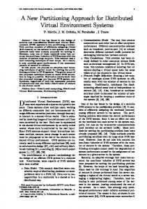
Consider the loop nest shown in Figure 1. The corresponding iteration space is shown in Figure 1(b). Note that the loop nest has a triangular geometry in the (i1 , i2 ) plane and a rectangular geometry in the (i1 , i3 ) plane. Assuming 3 processors are available, one can partition the outermost loop into three sets along the i1 -axis, as shown in Figure 2(a).2 The cardinality of the sets thus obtained is as follows (from left to right in Figure 2(a)): |S(1, 3)| = 18, |S(3, 5)| = 42 and |S(5, 7)| = 66, where S(x, y) = {i|x ≤ i1 < y}. However, one can interchange the loops corresponding to the loop indices i1 and i3 before partitioning. The sets thus obtained have equal cardinality, i.e., |S(1, 3)| = |S(3, 5)| = |S(5, 7)|, as shown in Figure 2(b). Unfortunately, in general, such partitioning may be impossible or impractical due to the following reasons: firstly, an equi-partitionable axis may not exist in a given N-dimensional convex polytope; secondly, determining functions for the loop bounds of the permuted loop is non-trivial. 1 2
Naturally, our technique can also handle rectangular loop nests too. Though an iteration space can be partitioned along an axis corresponding to an inner loop, however, it requires remapping of the index expressions (due to affine loop bounds) which introduces significant overhead. Therefore, we always partition an iteration space along the axis corresponding to the outermost loop.
2
do i1 = 1, N do i2 = 1, i do i3 = 1, N LOOP BODY end do end do
7 6 5 4 3 2 1
i3
7 6 7
5 6
end do
4
5 i2
(a) An example loop nest
4
3 3
2
i1
2 1
(b) Iteration space of loop nest shown in Figure 1(a), N = 6
Fig. 1. Partitioning non-rectangular iteration space
i2
i3
i1
i1
(a) Partitioning along i1 (Top view)
(b) Partitioning along i3 (Front view)
Fig. 2. Effect of geometry of an iteration space on partitioning
In practice, it is imperative to take into account the iteration space geometry to achieve a balanced work load distribution amongst the different sets of a partition. Also, the number of processors plays an important role in the efficient partitioning of a parallel loop nest. For example, we may partition the iteration space of Figure 1(b) across 4 and 5 processors. The corresponding partitions are shown in Figures 3(a) and 3(b) respectively. We observe that the size of the largest set (represented by boxes in Figures 3(a) and 3(b)) is the same in both the cases, and so is the execution time - if we exclude the scheduling overhead. However, unlike the partition in Figure 3(a), the partition of Figure 3(b) may incur additional scheduling overhead (e.g., communication due to an ex3
i2
i2
i1
i1
(a) P = 4
(b) P = 5
Fig. 3. Determining the number of processors (≤ P) for optimal performance based on the minimum size of the largest partition
tra processor and partition) with no performance gain. Thus, efficient processor allocation may also be important during iteration space partitioning.
3
Terminology
Let L denote a perfect nest of DOALL loops as shown in Figure 4. Without loss of any generality, we assume that the outermost loop is normalized from 1 to N with s1 = 1.3 The index variables of the individual loops are i1 , i2 , . . . , in and they compose an index vector i = (i1 , i2 , . . . , in ). An instance of the index vector i is an iteration. The set of iterations of a loop nest L is an iteration space Γ = {i}. We model an iteration space as a convex polytope in Zn . The lower and upper bounds (e.g., f3 and g3 , respectively) of an index variable (e.g., i3 ) are assumed to be affine functions of the outer loop indices (e.g., i1 and i2 ). We assume that fj ≤ gj for 1 ≤ j ≤ n − 1. The set of hyperplanes, defined by i1 = 1, i1 = N, ir = fr−1 and ir = gr−1 for 2 ≤ r ≤ n, determine the geometry of an iteration space. For example, if fr = lr and gr = ur where lr , ur ∈ Z (i.e., constant bounds) for 1 ≤ r ≤ n − 1, then the geometry of Γ is a rectangular parallelepiped. In this paper, we consider iteration spaces with complex geometries (e.g. tetrahedral, prismoidal) and with different, but constant, strides along each dimension. Of course, our technique can handle simpler, more regular loops as well. Definition 1. For each x, y ∈ R such that x < y, an elementary set S(x, y) in Γ is defined as follows : S(x, y) = {i|i ∈ Γ, x ≤ i1 < y}. 3
Note that the lower and upper bound of the outermost loop can be any two real numbers x, y ∈ R. Loops with real bounds are common in numerical applications [10] such as the Newton-Raphson method and Runge-Kutta method.
4
doall i 1 = 1, N, s1 doall i 2 = f1(i1 ),
g1(i1 ), s2
doall i n = fn−1(i1 , i 2 , ... , in−1 ), gn−1(i 1 , i 2 , ... , in−1 ), sn H(i) end doall end doall end doall
Fig. 4. A perfectly nested DOALL loop
Let β(Γ ) = {γk , k = 1, 2, . . . , m} denote a set of breakpoints of the outermost loop of L such that γ1 < γ2 2) degree polynomials as it is non-trivial to determine the closed form of their roots and is impossible for polynomial equations higher than fourth degree as stated by Abel’s Impossibility Theorem [31]. To alleviate this problem, we use binary search to determine the breakpoints. The solution of Equation (4) corresponds to the k th breakpoint γk . 6 In contrast, algebraic approaches [6,7,11] solve a system of P simultaneous equations to determine the breakpoints, which incurs significant overhead. The breakpoints thus obtained define the boundaries of the elementary sets in Γ . Note that unlike the approach presented in [7], the sets obtained by our approach are contiguous which eliminates the need for multiple loops, required in case of non-contiguous sets. Furthermore, contiguous sets facilitate exploitation of data locality. In contrast, previous approaches [6,7] balance load across different processors at the expense of data locality, as the sets obtained by applying these approaches are non-contiguous. 5
6
Assuming constant loop strides, partial volume is proportional to the number of index points in it. Note that V (x) is a monotonically increasing function of x. Therefore, there exists only one real solution of Equation (4).
6
Algorithm 1 Near-Optimal Partitioning of N-dimensional Non-Rectangular Iteration Spaces Input : An N-dimensional non-rectangular iteration space Γ and P processors. Output : A near-optimal (w.r.t. load balance amongst the different processors) partition of the iteration space. 0
/* Compute the partial volume V (x) of Γ */ V (x) =
Z
x
Z
g1
gn−1
Z ...
1
di1 di2 . . . din
f1
fn−1
/* Compute the total volume V of Γ */ V =
N
Z
Z
g1
gn−1
Z ...
1
f1
di1 di2 . . . din
(3)
fn−1
/* Determine the kth breakpoint γk . For 1 < k < (P − 1), determine the * * solution of Equation (4) using binary search */ V (γk ) =
k ×V P
(4)
β(Γ ) = {γ1 , γ2 , . . . , γP−1 } /* Eliminate void sets */ i ← 0, E ← 0 while i 6= |β(Γ )| do if bγi c = bγi+1 c then β(Γ ) ← β(Γ ) − {γi } i ← i − 1, E ← E + 1 end if i←i+1 end while /* Determine the loop bounds for the remaining P − E sets */ ( lbk =
1, ubk−1 + 1,
if k = 1 otherwise
(5)
γk − 1, ubk = bγk c, N,
if γk = bγk c if γk = 6 bγk c if k = P − E
where, lb and ub are the integer lower and upper bounds of an elementary set.
7
(6)
Next, we eliminate the void sets i.e. the sets which do not contain any index points and the corresponding breakpoints. The remaining sets are allocated to each processor. Given a minimum size of the largest set, the elimination process reduces the total number of sets which in turn minimizes the scheduling overhead. The (integer) lower and upper bounds of the loops corresponding to each set are determined using the equations 5 and 6 respectively. The algorithm is formally presented as Algorithm 1 on page 7. Note that, enumeration-based approaches may be used alternatively for computing the volume of a convex polytope. However, such techniques are not applicable in the presence of ceiling and floor functions in the loop bounds. 7 Furthermore, enumeration-based techniques such as [6,7] are not viable in the presence of non-unit strides. In fact, when the loop is normalized so that all index variables have unit stride, a non-linear constraint may appear in the loop bound. A similar problem is encountered during the data cache interference analysis for scientific computations. The non-linear constraint can be reduced to a linear one but with the introduction of further constraints. The authors of Omega Test and Polylib ([13,14]) formalize this transformation and propose a valid solution for the enumeration of rather complex iteration spaces. Nonetheless, the enumeration may be impractical for non-unit strides. In any case, our volumetric approach provides a simple, integrated and intuitive solution to the partitioning and processor allocation problem. Let us now examine the behavior of our algorithm on the example shown in Figure 1(a). First, we compute a partial volume of the convex polytope as a function of the outermost index variable. Next, we compute the volume of the convex polytope corresponding to the iteration space Γ . The total and partial volumes are given by : V =
N
Z
N
Z
di3 di2 di1 = 62.5 1
V (x) =
i1
Z
Z
x
1
Z
i1
1
Z
N
di3 di2 di1 = (N − 1) 1
1
1
(x − 1)2 2
Notice that alternatively, enumeration-based approaches may apply for the computation of volumes as follows: Ξ=
i1 N N X X X i1 =1
i2 =1
i3 =1
1 = N·
i1 N X X i1 =1
i2 =1
1= N·
N X i1 =1
i1 =
N 2 (N + 1) 2
Next, assuming 5 processors, we determine the breakpoints for the iteration space of Figure 1(b) are : 7
Floors and ceilings in loop bounds may arise after applying unimodular transformations [12]. Similarly, in many real applications, rational loop bounds can be found. In such cases, it is essential to convert the loop bounds to integers using the functions ceiling and floor.
8
i2 Void Set
i1 Eliminate
Fig. 5. Elimination of void sets
(γ1 − 1)2 1 (N − 1) = V 2 5
⇒ γ1 = 3.2,
(γ2 − 1)2 2 (N − 1) = V 2 5
⇒ γ2 = 4.1
(γ3 − 1)2 3 (N − 1) = V 2 5
⇒ γ3 = 4.8,
(γ4 − 1)2 4 (N − 1) = V 2 5
⇒ γ4 = 5.4
For simplicity, in this example we use the closed form of the roots of a quadratic equation to determine the breakpoints. Next, we eliminate the void sets i.e. the sets which do not contain any index points and the corresponding breakpoints, as shown in Figure 5. Next, we determine the lower and upper bounds of the remaining sets using the equations 5 and 6 respectively. The new loop bounds for the partition shown in Figure 5 are given by:
(lb1 , ub1 ) = (1, 4), (lb2 , ub2 ) = (4, 4), (lb3 , ub3 ) = (5, 5), (lb4 , ub4 ) = (6, 6) In the previous example, we assume that sets with equal volumes contain same number of iterations. It is important to note that the assumption is valid only if γi ∈ R ∀i. In presence of integer breakpoints, the iterations belonging to the corresponding boundary set must be allocated to either one adjoining elementary sets. This introduces load imbalance in the resulting partition. In Algorithm 1, we allocate such iterations to the elementary set on the right. For example, consider the iteration space shown in Figure 6. Assuming 3 processors, from Figure 6 we observe that γ1 , γ2 ∈ Z. The cardinality of the contiguous sets obtained from Algorithm 1 is 6, 8 and 10. Ideally, in this case the iterations in each boundary set must be distributed equally amongst the adjoining elementary sets in order to achieve perfect load balance. The boundaries corresponding to such a (optimal) partition is shown by dotted lines in Figure 6. However, such a distribution is not possible as the iteration space is partitioned only along the axis corresponding to the outermost loop. In the worst case, one might have to distribute the iterations in a boundary set 9
i2
4
4
γ1
6
γ2
9
i1
Fig. 6. Iteration space partitioning in presence of integer breakpoints
equally amongst different processors. We now present a bound on performance deviation of the partition obtained by Algorithm 1 from the optimal partition. Remark 1. Given any contiguous outermost partition Qβ(Γ ) determined by Algorithm 1, we have 0 ≤ T (Qβ(Γ ) ) − Topt (Γ, P) ≤
|Bγi | + |Bγi+1 | P γi ∈β(Γ )∩Z max
(7)
where, Topt (Γ, P) corresponds to the execution time of the optimal partition. Any elementary set Si ∈ Qβ(Γ ) is bounded by at most two hyperplanes i1 = γi and i1 = γi+1 . In Remark 1, if γi+1 ∈ / Z, then |Bγi+1 | = 0. So far, we have only considered perfect loop nests. However, our algorithm can be applied to multiway loop nests8 in a similar fashion. Likewise, our approach can be easily extended to handle non-constant strides. Detailed discussion of the above is outside the scope of this paper.
6
Experiments
To illustrate our algorithm’s behavior, we experimented with different loop nests taken from linear algebra packages and the literature. Table 1 lists the loop nests - the geometry of their iteration spaces and their source. The loops were partitioned using Algorithm 1. Subsequently, we refer to our approach as VOL and the canonical loop partitioning technique as CAN. First, we illustrate the effect of contiguous sets on performance. For the same, we partitioned loop L1 uniformly across P processors. Since L1 has rectangular geometry, both our approach and CAN result in the same number of iterations per processor. Thus, since both approaches have identical workload on each processor, the difference in performance, refer to Figure 7, can be attributed to 8
A loop is multiway nested if there are two or more loops at the same level. Note that the loops may be nested themselves[15].
10
#
Geometry
Source
L1 Rectangular SSYRK routine (BLAS3) L2 Tetrahedral
[7]
L3 Trapezoidal
Appendix A [16]
L4 Rhomboidal
Appendix A [16]
L5 Parallelepiped
pp. 58 [17]
Table 1. Geometries of the loop kernels. For each loop, N=1000.
Exploiting data locality during partitioning 16
CAN VOL
14
Execution time (s)
12 10 8 6 4 2 0
1
2
3 # of Processors
4
Fig. 7. Impact of data locality on performance of loop nest L1 (see Table 1)
data locality effects associated with contiguous sets, as explained in Section 5. Note that, our approach generates contiguous sets even with non-rectangular iteration spaces, thus facilitating exploitation of data locality in such iteration spaces as well. Next, we illustrate the performance of our algorithm for non-rectangular iteration spaces. For this, we determine the size (cardinality) of the largest set of partitions corresponding to each technique. Note that the size of the largest set in a partition correlates to the performance of that partitioning scheme. Table 2 presents the size of the largest set corresponding to our approach and (for comparison purposes) CAN. From Table 2 we observe that our approach results in smaller sizes of the largest set i.e. more uniform distribution of iterations across different processors. The difference in performance can be attributed to the fact that our approach accounts for the geometry of an iteration space during partitioning. We observe that the difference in performance decreases (expectedly) with increasing number of processors, as the volume of each set in a partition also decreases. As explained earlier, the applicability of CAN is restricted to canonical loops only, which explains the presence of dashes for loop nests L4 and L5 (noncanonical loop nests) for CAN. Furthermore, in case of large number of pro11
# of Processors 2
Loop Nest
VOL
4 CAN
VOL
8 CAN
VOL
16 CAN
VOL
CAN
L2 83368284 83596878 41810044 43807393 21003180 22397760 10738024 11538395 L3
476000
516000
219900
225037
109500
112056
55000
57232
L4
200000
-
100000
-
50000
L5
25000
-
12500
-
62500
-
25000
-
-
31500
-
Table 2. Performance (size of the largest set of a partition) of our geometric approach and canonical loop partitioning.
cessors, we also address processor allocation issues which eliminates the communication overhead due to extra processors and ensures efficient use of the processors.
7
Previous Work
It has been shown that loops without dependences among their iterations (traditionally known as DOALLs [18]) are a rich source of parallelism [19]. In addition, several compiler techniques [20] have been proposed to convert loops with interiteration dependences to DOALL loops for parallel execution. However, once this is done, the problem is how to partition the iteration space of the DOALLs across a given number of processors so as to minimize execution time and optimize processor utilization. In [21], Anik et al. discuss several models for parallel execution of nested loops. The simplest model is to execute the outermost loop in parallel and all the inner parallel loops sequentially. Another model involves collapsing [22] the nested loops into a single loop using compiler transformations. In another model, the inner loops are executed in parallel and a blocking barrier is used at the end of each parallel loop, which prevents the overlapping between execution of inner loops. Techniques such as loop concurrentization [23] partition the set of iterations of a loop and assigns a different subset to each processor. Irigoin and Triolet’s supernode partitioning approach [24] divides an iteration space of a loop nest into nodes with several goals : vector computation within a node, loop tiling for data reuse and parallelism between tiles. In [7], Sakellariou discusses the necessary condition for partitioning a loop nest across different processors with equal workload. Based on whether the iterations are distributed among processors before or during run-time, loop partitioning can be classified as static or dynamic. In static partitioning, each processor is assigned a fixed number of iterations such that the distribution among processors is as even as possible. The most common approaches for static partitioning are: 12
❐ Cyclic partitioning (CP) : It distributes the iterations in a round robin fashion; thus given n iterations and p processors, processor i executes iterations i + kp, k = 0, 1, . . . , n/p. However, this approach may deteriorate performance due to false sharing.9 ❐ Block partitioning (BP) [25] : This approach maps contiguous iterations onto processors in a consecutive manner; thus a processor i executes iterations in/p + 1 through (i + 1)n/p. The efficiency of BP is governed by the block size. Assuming zero scheduling overhead, the optimal block size is k = dn/pe number of iterations. ❐ Balanced chunk scheduling (BCS) [26] : BCS attempts to distribute the total number of iterations of the loop body among processors as evenly as possible as opposed to cyclic and block partitioning which distribute only the iterations of the outer loop. An example of the latter is shown in Appendix B of [7]. However, Haghighat and Polychronopolous restrict their discussion to double loops. ❐ Canonical loop partitioning (CLP) [7] : Sakellariou introduce a notion of canonical loop nest for loop partitioning. CLP assumes that the outermost loop can be equi-partitioned into 2pm−1 parts, where p is the number of processors and m is the depth of a loop nest. However, this may generate empty sets which leads to load imbalance. Moreover, CLP generates a fragmented partition i.e. each individual set is a collection of non-contiguous subsets. CLP employs an enumeration-based approach to determine the total number of index points in an iteration space. It relies on loop normalization in the presence of non-unit strides. However the introduction of floors and ceilings renders this approach nonviable in practice (see Section 5). Furthermore, determination of the set boundaries in CLP is very cumbersome. Similarly, Boyle et al. [11] present an approach for load balancing of parallel affine loops using unimodular transformations. Their approach transforms a loop into a load balanced form, i.e. it identifies an index variable ik , referred to as an invariant iterator, that neither makes any reference to any other index variable in its loop bounds, nor is referenced by any other index variable and reorders the iterations to move ik as far out as possible. However, this approach relies on the existence of an invariant iterator which restricts it’s applicability to rectangular iteration spaces only. Similarly, several techniques have been proposed in [27,28,29] for mapping affine loops on to multiple processors. However, these techniques focus primarily on communication minimization between the processors.
8
Conclusions
In this paper we presented an algorithm for partitioning N-dimensional iteration spaces. Unlike previous approaches [6,7], we follow a geometric approach for par9
False sharing occurs when multiple processors access data in the same cache line and one of the accesses is a ‘write’, thus causing the cache line to be exchanged between processors even though the processors access different parts of it.
13
titioning an iteration space. The partition thus obtained consists of contiguous sets, which facilitates exploitation of data locality. Our approach provides an integrated solution to the partitioning and processor allocation problems. Our experiments show that our approach has better performance than the CAN partitioning technique. As future work, we would like to extend our approach to partition iteration spaces at run-time.
9
Acknowledgments
The first author is highly grateful to Dr. Utpal Banerjee for the discussions, comments and suggestions which helped a lot in preparing the final version of the paper. He would like to thank Rafael Lopez, Carmen Badea and Radu Cornea for their help and feedback.
References 1. D. A. Padua. Multiprocessors: Discussion of theoritical and practical problems. Technical Report 79-990, Dept. of Computer Science, University of Illinois at Urbana-Champaign, November 1979. 2. R. Cytron. Doacross: Beyond vectorization for multiprocessors. In Proceedings of the 1986 International Conference on Parallel Processing, St. Charles, IL, August 1986. 3. J. Davies. Parallel loop constructs for multiprocessors. Technical Report 81-1070, Dept. of Computer Science, University of Illinois at Urbana-Champaign, May 1981. 4. C. Polychronopoulos, D. J. Kuck, and D. A. Padua. Execution of parallel loops on parallel processor systems. In Proceedings of the 1986 International Conference on Parallel Processing, pages 519–527, August 1986. 5. E. H. D’Hollander. Partitioning and labeling of loops by unimodular transformations. IEEE Trans. Parallel Distrib. Syst., 3(4):465–476, 1992. 6. Mohammad R. Haghighat and Constantine D. Polychronopoulos. Symbolic analysis for parallelizing compilers. ACM Transactions on Programming Languages and Systems, 18(4):477–518, July 1996. 7. R. Sakellariou. On the Quest for Perfect Load Balance in Loop-Based Parallel Computations. PhD thesis, Department of Computer Science, University of Manchester, October 1996. 8. U. Banerjee. Data dependence in ordinary programs. Master’s thesis, Dept. of Computer Science, University of Illinois at Urbana-Champaign, November 1976. Report No. 76-837. 9. M. Burke and R. Cytron. Interprocedural dependence analysis and parallelization. In Proceedings of the SIGPLAN ’86 Symposium on Compiler Construction, Palo Alto, CA, June 1986. 10. M.K. Iyengar, S.R.K. Jain, and R.K. Jain. Numerical Methods for Scientific and Engineering Computation. John Wiley and Sons, 1985. 11. M. O’Boyle and G. A. Hedayat. Load balancing of parallel affine loops by unimodular transformations. Technical Report UMCS-92-1-1, Department of Computer Science, University of Manchester, January 1992. 12. U. Banerjee. Loop Transformation for Restructuring Compilers. Kluwer Academic Publishers, Boston, MA, 1993.
14
13. W. Pugh. The Omega test: A fast and practical integer programming algorithm for dependence analysis. In Proceedings of Supercomputing ’91, Albuquerque, NM, November 1991. 14. P. Clauss and V. Loechner. Parametric analysis of polyhedral iteration spaces. In IEEE, editor, Int. Conf. on Application Specific Array Processors, Chicago, Illinois, August 1996. 15. C. Polychronopoulos. Loop coalescing: A compiler transformation for parallel machines. In S. Sahni, editor, Proceedings of the 1987 International Conference on Parallel Processing. Pennsylvania State University Press, August 1987. 16. S. Carr. Memory-Hierarchy Management. PhD thesis, Dept. of Computer Science, Rice University, September 1992. 17. U. Banerjee. Loop Parallelization. Kluwer Academic Publishers, Boston, MA, 1994. 18. S. Lundstrom and G. Barnes. A controllable MIMD architectures. In Proceedings of the 1980 International Conference on Parallel Processing, St. Charles, IL, August 1980. 19. D. Kuck et al. The effects of program restructuring, algorithm change and architecture choice on program performance. In Proceedings of the 1984 International Conference on Parallel Processing, August 1984. 20. M. J. Wolfe. Optimizing Supercompilers for Supercomputers. The MIT Press, Cambridge, MA, 1989. 21. S. Anik and W. W. Hwu. Executing nested parallel loops on shared-memory multiprocessors. In Proceedings of the 1992 International Conference on Parallel Processing, pages III:241–244, Boca Raton, Florida, August 1992. 22. M. J. Wolfe. High Performance Compilers for Parallel Computing. AddisonWesley, Redwood City, CA, 1996. 23. D. A. Padua and M. J. Wolfe. Advanced compiler optimizations for supercomputers. Communications of the ACM, 29(12):1184–1201, December 1986. 24. F. Irigoin and R. Triolet. Supernode partitioning. In Proceedings of the Fifteenth Annual ACM Symposium on the Principles of Programming Languages, San Diego, CA, January 1988. 25. C. P. Kruskal and A. Weiss. Allocating independent subtasks on parallel processors. IEEE Transactions on Software Engineering, 11(10):1001–1016, 1985. 26. M. Haghighat and C. Polychronopoulos. Symbolic program analysis and optimization for parallelizing compilers. In Proceedings of the Fifth Workshop on Languages and Compilers for Parallel Computing, New Haven, CT, August 1992. 27. N. Koziris, G. Papakonstantinou, and P. Tsanakas. Mapping nested loops onto distributed memory multiprocessors. In International Conference on Parallel and Distributed Systems, pages 35–43, December 1997. 28. M. Dion and Y. Robert. Mapping affine loop nests: new results. In HPCN Europe 1995, pages 184–189, 1995. 29. M. Dion and Y. Robert. Mapping affine loop nests. Parallel Computing, 22(10):1373–1397, 1996. 30. Matlab. http://www.mathworks.com. 31. Eric W. Weisstein. ”Abel’s Impossibility Theorem.” From MathWorld–A Wolfram Web Resource. http://mathworld.wolfram.com/AbelsImpossibilityTheorem. html.
15