Addison-Wesley Series in. Computer Science. Addison-Wesley, 1989. 4] Linda Stals. Parallel Multigrid on Unstructured Grids using Adaptive Finite Element ...
Computational Techniques and Applications: CTAC97 World Scienti c
1
A Key Based Parallel Adaptive Refinement Technique for Finite Element Methods S. Roberts
School of Mathematical Sciences, Australian National University, Canberra, ACT 0200, Australia.
S. Kalyanasundaram
Department of Engineering, Australian National University, Canberra, ACT 0200, Australia.
M. Cardew-Hall
Department of Engineering, Australian National University, Canberra, ACT 0200, Australia.
W. Clarke
Department of Engineering, Australian National University, Canberra, ACT 0200, Australia.
1. Introduction Many computational problems such as nite element analysis and computational
uid dynamics are solved by discretising the geometry of the problem into a mesh. Such problems may become very large. Splitting a geometry-based problem into small pieces and computing the solution all at once (parallel programming) should result in a much faster turnaround. Unfortunately these problems are not particularly conducive to such ne-grain parallelism since the solutions have many interdependencies, which means that there will be a great deal of inter-processor communication which slows computation. However, coarse-grain parallelism can be used e�ciently so long as each processor holds a large enough continuous piece of the mesh, and each processor sends and receives updates on the boundaries to and from its neighbours. To improve the accuracy of many such problems adaptive re nement may be used to re ne those parts of the mesh in which the accuracy is de cient. An important problem with parallel geometry-based programs is the decomposition of the mesh onto the processors: that is, determining which elements of the mesh go into which processor, such that the computation is evenly spread (load-balanced), and communication between processors is minimised. In addition, since adaptive re nement creates new elements the load quickly becomes unbalanced and so the mesh must again be decomposed and load-balanced. This paper investigates the use of spatial keys to uniquely identify and order the objects de ning a triangular mesh. By associating a key to each object in a mesh we obtain an order of the objects in one dimension. This makes decomposition much easier, since we simply divide the ordering into equal-sized pieces and let each processor have a piece. Keys based on the position ensure that objects which are close spatially generally have close key values, which tends to form decompositions with low communication costs. We present an adaptive re nement algorithm based on these ideas, and show typical parallel distributions of objects associated with di�erent keys.
2
S. Roberts, S. Kalyanasundaram, M. Cardew-Hall & W. Clarke n b 1
b 2
b Figure 1.
3 n
n 4 b n 4 1 1 b b
b2 b 3 3 2 b b 2 3 2 3 n n
Triangular re nement by newest-node bisection.
2. Re nement
A triangulation, or triangular mesh, is a collection of non-overlapping connected triangles. Such a triangulation is said to be conforming if every triangle's side is shared by exactly one neighbour | or zero neighbours on the boundary. For stable computations it is important that the triangles making up the mesh satisfy a minimal and maximal angle condition. For a given re nement algorithm and mesh, these set a lower and upper bound on the angles for any triangle. There are a number of basic types of triangular re nement, for instance: regular, centroidal and bisection. We will concentrate on newest-node bisection which works by giving each triangle a newest-node which is re ned. Figure 1 shows the rst four levels of newest-node re nement; vertices marked with an \n" are the newest nodes, sides marked with a \b" are the bases. The gure shows that there are four similarity classes of triangle produced for any given triangle, and hence the angle conditions are easily satis ed. It can be seen that given a side to re ne to, a triangle may re ne two levels at most to satisfy the re nement requirements. Both Mitchell [1] and Stals [4] use newest-node bisection in their respective nite element implementations. In our project we also use the newest-node bisection method as it allows local calculation of the re nement process and requires only a message notifying neighbouring elements that a re nement has taken place. In addition the method can be generalised to 3-dimensional meshes.
3. Key-Based Parallelism
When working with spatial data structures it is necessary to decide how to assign the structures to the processors. A standard method is to use domain decomposition where the whole structure is progressively divided into smaller and smaller pieces until each of the processors has a contiguous piece of the structure. This method takes time and a large amount of memory so other options were investigated. Samet [3, pp10{15] describes various methods for space-ordering and spatial data structures. He presents various mappings from 2-dimensional to 1-dimensional space including the Morton and Peano-Hilbert orders. The mappings are known as space lling curves because they pass through every point in the (integral) 2-dimensional parameter-space. The mappings preserve the spatial locality of the original set of objects. Figure 2 illustrates the Morton (M), Alternating Morton (M0), Peano-Hilbert
Key Based Finite Element Methods
3
(P H), and simple Concatenation orders (C ), which all de ne space lling curves in 2-dimensional parameter space. The M, M0 and C orders are speci ed by the key calculations (
x; y
)
=
( ?1 ?2 � � � 1 0 ?1 ?2 � � � 1 0)2 ( ?1 ?1 ?2 ?2 � � � 1 1 0 0 )2
M
!
(
x; y
xn
yn
xn
x x ; yn
yn
xn
yn
y y
) M! ( ?1 ?1 ?2 ?2 � � �
)
xn
C
!
=
yn
yn
( ?1 ?2 � � � �2 + yn
yn
n
y
(3.1)
y x y x
0
x; y
(
xn
xn
x1 y1 y0 x0
)2
(3.2)
?1 xn?2 � � � x1 x0 )2
(3.3)
y1 y0 xn
x
where ( ?1 ?2 � � � 1 0 )2 denotes the binary representation of an integer . The P H order is more complicated to specify and so we omit its speci cation due to lack of space. For our implementations of the key calculations we nd that the ratio of executions times is P H:M:M0 :C = 2.3:1:1:0.15. (These calculations were done on a SGI R4000 workstation, using gcc and g++ version 2.7.2). Due to the spatial properties of these keys, they form a good base for a decomposition. We can split the one-dimensional list of objects sorted by key into (approximately) equal pieces | where is the number of processors, and \equal" may be a weighted equality depending on the expected amount of work a given object will require. Warren and Salmon [5, 6] use a 3-dimensional Morton order key for N-body simulations. Stals [4, p69] uses a generalisation of the Morton order for global identi cation of nodes. Oden, Patra and Feng [2] use a Peano-Hilbert curve to order their quadrilateral elements. xn
xn
x x
x
p
p
4. Implementation Issues
The data structures that we use include the low-level elements of the mesh, as well as the containers which hold them. A mesh consists of three distinct parts, of increasing order (dimension-wise): the nodes (N ), the lines (L) which are the connections between the two end-point nodes and between two neighbouring triangles (parents); and the triangles (T ) which signify a connected triple of lines. In order to refer between objects of a mesh, we must either have direct references or some other method of determining the location of an object. Since the particular object to be referenced may be on a di�erent processor, we cannot have direct references (such as pointers). We could use its \location" in 2- or 3-dimensional space, but this does not enable quick access within a processor. Storage via keys enables the use of hash-tables or search-trees in order to access the required object quickly. In order to make the mapping from coordinates to keys one-to-one, we rst represent the coordinates of objects as (unsigned) integers. This means that if we are given the coordinates in oating point we must convert them to integral coordinates.
4
S. Roberts, S. Kalyanasundaram, M. Cardew-Hall & W. Clarke y
y
7
7
6
6
5
5
4
4
3
3
2
2
1
1
0
0 0
1
2
3
4
(a)
5
6
7
x
y
y
7
7
6
6
5
5
4
4
3
3
2
2
1
1
0
0
1
2
3
4
5
6
7
x
0
1
2
3
4
5
6
7
x
(b)
0 0
1
2
3
4
(c)
5
6
7
x
(d)
(a) The Morton, (b) the Alternating Morton, (c) the PeanoHilbert and (d) the Concatenate orders through 3-bit coordinate space.
Figure 2.
This is done by scaling the coordinates of the objects so that the coordinates di�er in at least one dimension by one. Then the closest point in Z2 provides the integer coordinates of an object. If the initial mesh is given as a set of connected points or nodes then the integral coordinates of the set of nodes are rst calculated. After that, in order to specify the integral coordinates for each line we specify the mid-point of each connection as the \coordinates" of each line. The obvious coordinates of a triangle is its centroid, but this leads to divisions by 3. With newest-node bisection, another obvious choice is the mid-point of the bisector. When re ning we replace a line with a new node (at the location of that line) and two new lines (with locations at the midpoints of the new node and the original end-points). We also bisect a triangle, replacing it with a new line (at the location of that triangle) and two new triangles (with locations at the midpoint of the new node and the opposite side). This means that the integral distance of each distinct type (node, line and triangle) will divide by two. However, during re nement it is possible for there to be two levels of triangles and lines created; this means in general each re nement process will divide the mesh integral distance by four. Each of the mesh objects has slightly di�erent requirements and structures:
Key Based Finite Element Methods
Figure 3.
�
5
Mesh example: L-shaped domain.
the only relevant feature of a node is its location; i.e. a node N = f g, where is the location; a line consists of a location, two end-points and two parents (where one of the parents may not exist); i.e. a line L = f f 1 2 g f 1 2 gg, where is the location (de ned as the midpoint between end-points 1 and 2), is the key of an end-point, and is the key of a parent; we order the keys of the end-points such that 1 2 to aid re nement; and a triangle consists of a location, three corners and three sides; i.e. a triangle T = f f 1 2 3 g f 1 2 3 gg, where is the location (de ned as the midpoint of the newest node 1 and the oldest side 1), is the key of a corner and is the key of a side; the keys of the second and third corners are ordered such that 2 are ordered such that they are opposite the 3 , and the sides corresponding corner . n
n
�
l;
e ;e
;
e
p ;p
l
e
ei
pi
ei
�
e
t;
< e
c ;c ;c
;
s ;s ;s
t
c
c
s
< c
ci
si
si
ci
Each object in the mesh has an integral coordinate. It may also have references to other objects within the mesh via those objects' keys. This means that we must be able to e�ciently access an object within the mesh given its key. Such a problem is well-suited to hash-tables and search-trees. The C++ Standard Template Library (STL) provides a standard set of associative containers which enable one to associate an object of a given class with that of an ordered class (in which the ordering is entirely up to the user). This project uses STL in its implementation of the algorithms however, the principles will apply to any other container which quali es.
5. An Example
Using an initial coarse L-shaped mesh up of four triangular elements as illustrated in Figure 3, we will demonstrate the behaviour of the key-orders and the adaptive re nement algorithm. The criterion used for adaptive re nement of the L-shaped mesh tries to mimic the behaviour of nite element error indicators applied to the solution of Laplace's equation on a domain with a re-entrant corner. So for a given tolerance we specify T
6
S. Roberts, S. Kalyanasundaram, M. Cardew-Hall & W. Clarke
that the length of any line in the mesh satis es h
hr
? 31
(5.1)
< T
where is the distance of the line from the re-entrant corner. For this example the large side length is 32,768 and a tolerance = 50 produces 8 levels of re nement where the last four levels of re nement are truly adaptive. The sixth level of re nement of the L-shaped domain load-balanced over four processors for each of the Morton, Peano-Hilbert and Concat key-orders are shown in Figures 4, 5 and 6 respectively. Boundary statistics are used to measure the \goodness" of the decomposition. We measure the number and length of lines which have nodes or parents on di�erent processors. Similarly we measure the number and area of triangles which have components which \live" on di�erent processors. These boundary statistics are summarised in Table 1, and this shows that all three key-orders produce similar distributions, with the Peano-Hilbert order distribution tending to be slightly better. r
T
Figure 4.
L-shaped Domain, = 4, 6th level: Morton order. P
While we have not tested three-dimensional meshes, one would suspect that the Morton and Peano-Hilbert orders would work much better than the Concat order.
6. Conclusion
We have shown that a spatial key can be used to uniquely identify and order all objects of a triangular mesh. The key also provides a simple method to decompose
Key Based Finite Element Methods
Figure 5.
7
L-shaped Domain, = 4, 6th level: Peano-Hilbert order. P
Measure: No. lines Line length No. triangles Triangle area M 192 128467 351 6.001e7 PH 168 122923 339 6.521e7 P H/M% 87.5 95.7 96.6 108.7 C 210 144291 282 5.741e7 C /M% 109.4 112.3 80.3 95.7 O
Table 1.
Boundary measure for L-shaped domain, = 4, 6th level. P
the mesh over the processors. A parallel adaptive re nement algorithm with load balancing has been successfully implemented and some results presented. The data structures, adaptive re nement and load-balancing implementation form a powerful parallel C++ library which can be adapted for use in computational engineering codes. The code uses the C++ Standard Template Library for mesh storage and the Message Passing Interface for parallel programming.
7. Acknowledgements
This work was supported by Australian National University Faculty Research Grants, F97128 \Computational Modelling and Simulation of Advanced Manufacturing Systems", and FNS-06 \Parallel Adaptive Meshing Techniques for Finite Element
8
S. Roberts, S. Kalyanasundaram, M. Cardew-Hall & W. Clarke
Figure 6.
L-shaped Domain, = 4, 6th level: Concat order. P
Methods".
References
[1] William F. Mitchell. Uni ed Multilevel Adaptive Finite Element Methods for Elliptic Problems. PhD thesis, University of Illinois, Urbana-Champaign, 1988. [2] J. Tinsley Oden, Abani Patra, and Yusheng Feng. Domain decomposition for adaptive hp nite element methods. In David E. Keyes and Jinchao Xu, editors, Domain Decomposition Methods in Scienti c and Engineering Computing, volume 180 of Contemporary Mathematics, pages 296{ 301, Pennsylvania State University, 1993. NSF, US DoE, IMA, GAMNI, American Mathematical Society, Rhode Island. [3] Hanan Samet. The Design and Analysis of Spatial Data Structures. Addison-Wesley Series in Computer Science. Addison-Wesley, 1989. [4] Linda Stals. Parallel Multigrid on Unstructured Grids using Adaptive Finite Element Methods. PhD thesis, ANU Department of Mathematics, Australia, June 1995. [5] M. S. Warren and J. K. Salmon. A parallel hashed oct-tree n-body algorithm. In Supercomputing '93, pages 12{21, Los Alamitos, 1993. IEEE Comp. Soc. [6] M. S. Warren and J. K. Salmon. Abstractions and techniques for parallel n-body simulations. In Parallel Object Oriented Methods and Applications (POOMA) '96, 1996.