A Low Computation Cost Algorithm to Solve. Cellular Systems with Retrials Accurately. Ma José ... orbit and retries after an exponentially distributed time with rate µr. .... The generic definition of the state space of that Markov process is S :=.
A Low Computation Cost Algorithm to Solve Cellular Systems with Retrials Accurately Ma Jos´e Dom´enech-Benlloch, Jos´e Manuel Gim´enez-Guzm´an, Jorge Mart´ınez-Bauset and Vicente Casares-Giner Department of Communications, Universitat Polit`ecnica de Val`encia, UPV ETSIT Cam´ı de Vera s/n, 46022, Val`encia, Spain {mdoben,jogiguz}@doctor.upv.es,{jmartinez,vcasares}@dcom.upv.es
Abstract. This paper proposes an approximate methodology for solving Markov models that compete for limited resources and retry when access fails, like those arising in mobile cellular networks. We limit the number of levels that define the system by aggregating all levels beyond a given one in order to manage curse of dimensionality issue. The developed methodology allows to balance accuracy and computational cost. We determine the relative error of different typical performance parameters when using the approximate model as well as the computational savings. Results show that high accuracy and cost savings can be obtained by deploying the proposed methodology.
1
Introduction
A common assumption when evaluating the performance of communication systems is that users that do not obtain an immediate service leave the system without retrying. However, due to the increasing number of users and the complexity of current systems the impact of retrials is no longer negligible. This perception has triggered an increasing interest in introducing the phenomenon of retrials in telecommunication systems. Different models have been proposed to evaluate the impact of blocked subscribers retrying after a relative short delay, both in wire line telephone networks [1] and in cellular networks [2]. The retrial phenomenon can also be observed in web browsing, where users try to reload a web page in case of congestion. Retrials do not only appear as a consequence of user behavior, but also due to the operation of some protocols like random access protocols [3]. For an interesting overview of the retrial phenomenon, please refer to [4] and references therein. In real systems, the population can be very large or even infinite, so the numerical computation can become extremely large in terms of memory space and CPU time, or even impossible in many cases. So approximate methodologies are needed like the one proposed in [5], which is studied in a mobile cellular network scenario. It is based on grouping states according to the presence or not of users in the retrial orbit. Our work is motivated by the perception that this seems a gross approximation in overloaded systems, where retrials are specially
2
Fig. 1. System Model.
critical. As it will be shown later, the precision with which common performance parameters are estimated can be quite poor. Our proposal makes it possible a gradual transition from the model in [5] towards the exact model. The rest of the paper is structured as follows. Section 2 describes the exact model and defines the performance parameters, comparing it with the approximation proposed in [5]. Section 3 introduces the novel approximation of the Markov model and Section 4 presents its numerical evaluation. Finally, a summary of the paper and some concluding remarks are given in Section 5.
2
System Model
As in [5], the system under study is a mobile cellular network with customer retrials. This system can be modeled by Fig. 1, where a group of M users contend for C servers, requesting an exponentially distributed service time with rate µ. When a user accesses the system and finds all servers busy, it joins the retrial orbit and retries after an exponentially distributed time with rate µr . The retry is successful if it finds a free server. Otherwise, the user returns to the retrial orbit with probability (1 − Pi ) or leaves the system with probability Pi . The implicit assumption of geometric distribution for the number of retrials is a first order approximation to more exact models like the one proposed in [6]. The arrival process is modeled as an state-dependent Poisson process with rate λ(k, m) = (M − k − m)λ, being λ the individual user arrival rate when idle, and k (m) the number of users in service (in the retrial orbit). The most common performance parameter used in queueing systems is the blocking probability, which is defined as the probability of having all servers occupied. Notwithstanding, other performance parameters can describe the behaviour of retrial systems more accurately. That performance parameters are the immediate service probability (Pis ), the delayed service probability (Pds ) and the non-service probability (Pns ). Obviously, it must be met that Pis +Pds +Pns = 1. The computation of such performance parameters can be done in terms of the next rates. Let us denote by Ro the mean offered user rate, by R1,s the mean
3
Fig. 2. Exact Markov model.
first attempt successful rate and by R1,f the mean first attempt failure rate. It is obvious that, Ro = R1,s + R1,f . Let us also denote by Rr the mean retrial rate, by Rr,s the mean successful retrial rate, and by Rr,f the mean failure retrial rate. It is also obvious that, Rr = Rr,s + Rr,f . Finally, let us denote by Rab the mean abandon rate, which can be expressed as Rab = Pi Rr,f . The performance parameters are defined by the following expressions Pis = 2.1
Rr,s Rab R1,s ; Pds = ; Pns = Ro Ro Ro
(1)
Exact Markov model
The retrial system described in Fig. 1 can be modeled as a Markov process with the state space defined as S := {(k, m) : 0 ≤ k ≤ C; 0 ≤ m ≤ M − C}, where k is the number of occupied servers and m the number of users in the retrial orbit. The state-transition diagram is shown in Fig. 2. The infinitesimal generator matrix (2) presents a tridiagonal structure whose elements are also matrices. This is the classical structure of a QBD process [7].
D0 M1 0 . Q= .. 0 0 0
L0 D1 M2 .. . 0 0 0
... 0 0 ... 0 0 ... 0 0 . . .. . . . . . . . . LM −C−2 0 . . . DM −C−1 LM −C−1 . . . MM −C DM −C
(2)
4
where Mm , Dm and Lm , are square matrices with dimension (C + 1)(C As an example, for C = 5 we have 00000 0 0 mµr 0 0 0 0 0 0 0 0 0 0 0 0 mµr 0 0 0 00000 0 0 0 0 mµ 0 0 r Lm = Mm = 0 0 0 0 0 0 0 0 mµr 0 0 0 0 0 0 0 0 0 0 0
0 0
0 0
0 0
0 0
mµr mµr Pi
0 0 0 0 0 λ(5, m)
Dm
0 0 0 ∗ λ(0, m) µ ∗ λ(1, m) 0 0 ∗ λ(2, m) 0 = 0 2µ 0 0 3µ ∗ λ(3, m) 0 0
0 0
0 0
+ 1).
4µ 0
∗ 5µ
0 0 0 0 λ(4, m) ∗
The asterisks that appear in Dm are the negative values that make the sum of every row of Q equal to zero. The stationary state probability vector π can be obtained by solving πQ = 0 with the normalization condition πe = 1. Note that e is the common all ones transposed vector. The blocking probability can be computed as BP =
M−C X
π(C, m)
m=0
And the rest of the performance parameters can be determined by using the following expressions Ro =
C M−C X X
λ(k, m)π(k, m)
C−1 X M−C X
λ(k, m)π(k, m)
Rr =
k=0 m=0
R1,s =
M−C X
λ(C, m)π(C, m)
m=0
2.2
mµr π(k, m)
C−1 X M−C X
mµr π(k, m)
k=0 m=0
Rr,s =
k=0 m=0
R1,f =
C M−C X X
k=0 m=0
Rr,f =
M−C X
mµr π(C, m)
m=0
Previous approximate Markov models
In [5] a boolean variable is defined to indicate the presence (’1’) or absence (’0’) of blocked users with option to retry. Then, the approximation is done by aggregating all the columns of the exact model beyond the first one, i.e. aggregating states depending on the presence or not of users in the retrial orbit. We evaluated the error introduced by this approximation in a mobile cellular network scenario, which parameters are similar to the ones used in [5], being
5
M C µ λ ) ρ (ρ = λ+µ µr Pi
120 users 30 servers 1/180s−1 0.14 — 0.44 0.1s−1 0.5
The results for the exact Markov model are presented in Fig. 3(a), where we show the evolution of the different performance parameters as ρ increases. As can be seen, retrials become important when the system is overloaded, i.e. when the blocking probability is, for example, over 10% (ρ ≃ 0.22). In Fig. 3(b) we evaluate the relative error in the performance parameters when using the approximate methodology, defined by | Γ exact −Γ approx | /Γ exact , where Γ ∈ {BP, Pis , Pds , Pns }. As shown, the blocking probability computed by the approximate model is close to its exact value. However, the relative error in the rest of the performance parameters is not negligible when the mean number of users in the retrial orbit is significant, i.e. in overloaded systems. 1
0.7 BP Pis Pds Pns
0.9 0.6
0.5
0.7 0.6
|Pexact−Paprox|/Pexact
Performance parameters
0.8
BP P is Pds P
0.5
ns
0.4 0.3
0.4
0.3
0.2
0.2 0.1
0.1 0
0.15
0.2
0.25
ρ
0.3
0.35
0.4
(a) Results of the exact Markov model.
0
0.15
0.2
0.25
ρ
0.3
0.35
0.4
(b) Relative errors respect to the exact.
Fig. 3. Results of the exact model and relative errors of the approximate model.
3
Novel approximate Markov model
We propose a novel approximate Markov model that is able to improve the accuracy of the model proposed in [5], with a relatively small additional computation cost. This novel model can be considered a generalization of [5], being the aggregation done when there are Q or more users in the retrial orbit. The value of Q is tunable from Q = 1 (as proposed in [5]) to Q = M − C (exact model), increasing both accuracy and computation cost as we increase Q. The generic definition of the state space of that Markov process is S := {(k, m) : 0 ≤ k ≤ C; 0 ≤ m ≤ Q}, where k is the number of occupied servers and
6
Fig. 4. Approximate Markov model.
m (when m < Q) is the number of users in the retrial orbit. The set of states (k, Q) corresponds to the situation where Q or more users are in the retrial orbit. Fig. 4 shows the state transition diagram of the proposed approximate model. The first Q − 1 columns are exactly the same as the first Q − 1 columns in Fig. 2. For column Q we approximate the new users arrival rate by λ(k, Q) = (M − k − m)λ, where m denotes the average number of users in the retrial orbit when it holds Q or more users. When a user in the retrial orbit executes a successful retrial, then the number of users in the orbit can drop below Q with probability (1 − p) or not with probability p. Therefore, the retrial rate in states (k, Q) could be split in two contributing rates α and β. The first one corresponds to transitions from (k, Q) to (k + 1, Q − 1) and is approximated by α = mµr (1 − p). The second one corresponds to transitions from (k, Q) to (k + 1, Q), and is approximated by β = mµr p. Parameters m and p must be conveniently estimated from the model.
The infinitesimal generator of the proposed model Q presents the same structure as the exact model infinitesimal generator changing the limits from (M −C) to Q. Matrices MQ and DQ are different from those defined in the exact model. As an example, for C = 5 we have
7
0α0 0 0 0 ∗ λ(0, m) + β 0 0 α 0 0 0 µ ∗ 0 0 0 α 0 0 0 2µ MQ = DQ = 0 0 0 0 α 0 0 0 0 0 0 0 0 α 0 0 0 0 0 0 0 αPi 0 0 The rates defined in Section 2 can now be rewritten as Ro =
R1,s =
Q C X X
mµr π(k, m) + mµr
k=0 m=0
C Q−1 X X
k=0 m=0
Q X
C−1 X Q−1 X
mµr π(k, m) + mµr
C−1 X
λ(k, m)π(k, m)
λ(k, m)π(k, m)
Rr =
Rr,s =
k=0 m=0
R1,f =
... 0 ... 0 ... 0 ... 0 . . . λ(4, m) + β ... ∗
Q X
C X
k=0 m=0
λ(C, m)π(C, m)
Rr,f =
m=0
Q−1 X
π(k, Q)
k=0 C−1 X
π(k, Q)
k=0
mµr π(C, m) + mµr π(C, Q)
m=0
Parameters p and m can be estimated as described below. Balancing the probability flux crossing each vertical cut of the state transition diagram produces the following set of equations λ(C, 0)π(C, 0) = µr
C X
π(k, 1) − µr π(C, 1) + µr Pi π(C, 1)
k=0
λ(C, 1)π(C, 1) = 2µr
C X
π(k, 2) − 2µr π(C, 2) + 2µr Pi π(C, 2)
(3)
k=0
... λ(C, Q − 1)π(C, Q − 1) = mµr (1 − p)
C X
π(k, Q) − mµr (1 − p)(1 − Pi )π(C, Q)
k=0
Summing them we obtain X
Q−1
X
Q−1
λ(C, m)π(C, m) =
m=0
+ mµr (1 − p)
mµr
m=0 C X
C−1 X k=0
X
Q−1
π(k, m) + Pi
mµr π(C, m)
m=0
π(k, Q) − mµr (1 − p)(1 − Pi )π(C, Q)
k=0
This equation can be rewritten as �
�
�
R1,f − λ(C, Q)π(C, Q) = Rr,s − mµr
C X
�
π(k, Q) + mµr π(C, Q) +
k=0
�
�
+ Rab − mµr Pi π(C, Q) + mµr (1 − p)
C X k=0
π(k, Q) − mµr (1 − p)(1 − Pi )π(C, Q)
8
Given that R1,f = Rr,s + Rab and after some algebra we get λ(C, Q)π(C, Q) = mµr p
C X
π(k, Q) − mµr p(1 − Pi )π(C, Q)
(4)
k=0
From (3) and (4) we get p=
λ(C, Q)π(C, Q) λ(C, Q − 1)π(C, Q − 1) + λ(C, Q)π(C, Q)
(5)
λ(C, Q − 1)π(C, Q − 1) + λ(C, Q)π(C, Q) Pk=C−1 µr [ k=0 π(k, Q) + Pi π(C, Q)] To find the values of p and m an iterative procedure must be followed. Starting with p = 0 and m = Q the stationary state probabilities π(k, m) can be computed and the next values for p and m obtained. The procedure is repeated until the relative precision is less than, for example, 10−4 . In [5] the convergence of the iterative procedure was assumed. We evaluated a wide range of scenarios with different configuration parameters and the procedure converged in all cases. m=
4
Numerical Evaluation
This section has a two-fold objective. One is to evaluate the accuracy of our approach and the other is to evaluate the computation cost savings that can be obtained when referring to the exact model. The parameters used in the scenario under study are the ones presented in Section 2. 4.1
Accuracy
In this section, we study the relative error in the performance parameters for approximate models with increasing complexity, i.e. with an increasing Q value. In Fig. 5 we plot the relative error in the performance parameter values for different loads. In general, the relative error in all performance parameters decreases as we get closer to the exact model, i.e. as Q increases. Note again that using Q = 1 might not be a good choice because the relative error in Pis , Pds and Pns is not negligible. It can be noted that the degree of success of approximations in systems with retrials is mainly dependent on the offered load. The reason of this behavior is that as more load is offered more users will be held in the retrial orbit. Therefore, using higher values for Q seems an intuitive choice. However the value of Q required for a given precision is much lower than (M − C), that would constitute the exact solution. For example, in the worst scenario studied (ρ = 0.44), with Q = 12 we can get a relative error of less than 10−2 in the worst performance parameter while reducing the number of states more than 85%. In not so overloaded scenarios, the state space reduction is even higher. As a conclusion, a rule of thumb to determine a suitable value for Q could be to try with a value around Q ≃ 0.15(M − C), independently of the system load, although lower values would be probably enough. We have checked this rule in several scenarios and we found that it was a good choice in all of them.
9 0.1
0.3 Q=1 Q=3 Q=6 Q=9 Q=12
0.09
exact
0.08
Q=1 Q=3 Q=6 Q=9 Q=12
0.25
0.2
is
|Pexact−Paprox|/Pexact
exact
0.06 0.05
0.15
is
−BP
aprox
|/BP
0.07
|BP
is
0.04
0.1
0.03 0.02 0.05 0.01 0
0.15
0.2
0.25
ρ
0.3
0.35
0
0.4
(a) Blocking probability.
0.2
0.25
ρ
0.3
0.35
0.4
(b) Immediate service probability.
0.7
0.7 Q=1 Q=3 Q=6 Q=9 Q=12
0.6
Q=1 Q=3 Q=6 Q=9 Q=12
0.6
0.5 ns
ds
|Pexact−Paprox|/Pexact
0.5
|Pexact−Paprox|/Pexact
0.15
0.4
ns
ds
0.4
0.3
ns
ds
0.3
0.2
0.2
0.1
0.1
0
0.15
0.2
0.25
ρ
0.3
0.35
0.4
(c) Delayed service probability.
0
0.15
0.2
0.25
ρ
0.3
0.35
0.4
(d) Non-service probability.
Fig. 5. Relative errors respect to the exact.
4.2
Computation Costs
In this section we compare the computation costs, measured in floating-point operations (flops),1 required to solve the exact and approximate models. Two different algorithms have been used, the GJL’s proposed by Gaver, Jacobs and Latouche in [8] and the Servi’s algorithm proposed in [9]. They provide the same solution but they need a different number of flops. The scenario considered uses a load of ρ = 0.22, which is a typical overloaded scenario. For this scenario it is sufficient to consider Q = 6, as can be shown in Fig. 5. Fig. 6(a) shows the cost of each solving algorithm when applied to both the exact and the approximate models with a required relative precision of 10−4 for the computation of m and p. It is clear that the Servi’s algorithm outperforms the GJL’s algorithm for the range of Q values of interest. Note that 1
The numerical results and their associated computation cost have been obtained using Matlab. For this product, sums and subtractions require 1 flop if operators are real and 2 flops if complex, products and divisions require 1 flop if the result is real and 6 flops otherwise.
10 6
10
0.7
0.6
5
Flops x 1e3
4
10
3
10
Approx Model Servi’s Alg. Approx Model GJL’s Alg. Exact Model GJL’s Alg. Exact Model Servi’s Alg.
2
10
% Operations respect to the exact
10
0.5
0.4
0.3
0.2
0.1
1
10
10
20
30
40
50
60
70
80
Q
(a) Computation costs with different algorithms.
0 1
2
3
4
5 Q
6
7
8
9
(b) Computation cost for the algorithm 0 proposed by Servi.
Fig. 6. Results of the exact model and relative errors of the approximate model.
the value of Q at which the costs of the approximate and exact models become equal is less than M − C, and from this point on the cost of the approximate model is higher than the cost of the exact model. This is due to the fact that the approximate model has an additional overhead associated to the iterative computation of m and p. For Servi’s algorithm, Fig. 6(b) displays the ratio of the costs of solving the approximate and the exact model. As shown, computation costs savings of approximately 99.6% are possible for Q = 6, which constitute a substantial performance gain while guaranteeing excellent precision. Moreover, additional savings can be obtained when using a smaller precision for the estimation of m and p. Fig. 7(a) shows the variation of the relative error of the performance parameter which exhibits the highest error (Pds ) as a function of Q. It is clear that for values of Q higher than 6, it is enough to use rough estimations of m and p to achieve a negligible relative error for the values of the performance parameters. Fig. 7(b) shows the ratio of the costs of solving the approximate and the exact model as a function of Q. As observed, the computation cost can additionally be reduced by a factor of 2 for typical values of Q when using rough estimations of m and p.
5
Conclusions
We have proposed a novel methodology to determine the value of typical performance parameters in systems with retrials like mobile cellular networks. In these systems, repeated calls can have a negative impact on the performance and therefore its evaluation should not be neglected in the phases of design and planning. When the computation of the exact model might not be feasible due to the explosion of the state space, approximate methodologies are needed.
11 0.7
0.14
0.6 % operations respect to the exact
Precision=0.0001 Precision=0.001 Precision=0.01 Precision=0.1
0.12
Relative error
0.1
0.08
0.06
0.04
0.5
0.4
0.3
0.2
0.1
0.02
0 1
Precision=0.0001 Precision=0.001 Precision=0.01 Precision=0.1
2
3
4
5 Q
6
7
8
9
(a) Relative error of the performance parameter which exhibits the highest error (Pds ).
0 1
2
3
4
5 Q
6
7
8
9
(b) Computation cost for the algorithm 0 proposed by Servi.
Fig. 7. Effect of using different precisions for the estimation of m and p.
Our approximation methodology substantially improves the precision of previous approximations like [5], when estimating critical performance parameters. The computation cost can be reduced by two orders of magnitude when comparing to the exact model for a typical overloaded scenario. Additionally, it requires only a very small computation cost increase when compared to the model of [5]. We have noted that relative errors are very sensitive to the load offered to the system, being higher as load increases. We have shown that with a state space reduction of 85% respect to the exact model, our methodology is able to achieve accurate solutions, even in overloaded scenarios. At present authors are extending this model by considering several retrial orbits. Here, the proposed methodology will allow to handle the state space explosion.
Acknowledgment The authors express their sincere thanks to Jes´ us Artalejo and Vicent Pla for their insightful comments. This work has been supported by the Spanish Government and the European Commission through projects TIC2003-08272 and TEC2004-06437-C05-01 (30% PGE and 70% FEDER), by the Spanish Ministry of Education and Science under contract AP-2004-3332 and by the Universidad Polit´ecnica de Valencia under Programa de Incentivo a la Investigaci´on.
References 1. K. Liu, Direct distance dialing: Call completion and customer retrial behavior, Bell System Technical Journal, Vol. 59, pp. 295–311, 1980.
12 2. P. Tran-Gia and M. Mandjes, Modeling of customer retrial phenomenon in cellular mobile networks, IEEE Journal on Selected Areas in Communications, Vol. 15, pp. 1406–1414, October 1997. 3. D. J. Goodman and A. A. M. Saleh, The near/far effect in local ALOHA radio communications, IEEE Transactions on Vehicular Technology, Vol. 36, no. 1, pp. 1927. February 1987. 4. J. Artalejo and G. Falin, Standard and retrial queueing system: A comparative analysis, Revista Matem´ atica Complutense, vol 15, no. 1 pp. 101-129, 2002. 5. M. A. Marsan, G. De Carolis, E. Leonardi, R. Lo Cigno and M. Meo, Efficient Estimation of Call Blocking Probabilities in Cellular Mobile Telephony Networks with Customer Retrials, IEEE Journal on Selected Areas in Communications, Vol. 19, no. 2, pp. 332-346, February 2001. 6. E. Onur, H. Deli¸c, C. Ersoy and M. U. C ¸ aglayan, Measurement-based replanning of cell capacities in GSM networks, Computer Networks, Vol. 39, pp. 749-767, 2002. 7. M. F. Neuts, Matrix Geometric Solutions in Stochastic Models: An Algorithmic Approach, The John Hopkins University Press, Baltimore, 1981. 8. D. P. Gaver, P. A. Jacobs and G. Latouche, Finite birth-and-death models in randomly changing environments, Advanced Applied Probability, Vol. 16, pp. 715-731, 1984. 9. L. D.Servi, Algorithmic Solutions to Two-Dimensional Birth-Death Processes with Application to Capacity Planning, Telecommunication Systems, Vol. 21:2-4, pp. 205212, 2002.