Progress In Electromagnetics Research B, Vol. 55, 87–114, 2013
A MULTI-FIDELITY BASED ADAPTIVE SAMPLING OPTIMISATION APPROACH FOR THE RAPID DESIGN OF DOUBLE-NEGATIVE METAMATERIALS Patrick J. Bradley RF & Microwave Research Group, School of Electrical Electronic and Communications Engineering, University College Dublin, Ireland Abstract—Due to the increasing complexity of metamaterial geometric structures, direct optimisation of these designs using conventional approaches, such as Gradient-based and evolutionary algorithms, are often impractical and limited. This is in part due to the inherently high computational cost associated with running multiple expensive high-fidelity full-wave simulations, commonly required to optimise the constitutive parameters of a single metamaterial particle. In order to alleviate this issue, we propose an efficient optimisation approach which exploits the Co-Kriging methodology, such that we can successfully couple varying levels of discretisation and solver accuracy obtained from a 3d full-wave numerical solver suite. In contrast to other optimisation strategies, we investigate the improvement in efficiency of optimisation through the use of the LOLA-Voronoi, in conjunction with Expected Improvement and the embedding of a trustregion framework within our optimisation algorithm, to accelerate the convergence of Co-Kriging. Finally, the effectiveness of the outlined algorithm will be demonstrated by a quantitative evaluation of the performance of optimised planar 2D negative index of refraction structures. 1. INTRODUCTION The ability to independently tailor the electric and magnetic response of sub-wavelength geometric structures to electromagnetic energy, has provided the opportunity for designers to create fully customised artificial materials termed Metamaterials. These structures allow for fully tuneable material properties that can be engineered to have Received 10 July 2013, Accepted 23 September 2013, Scheduled 24 September 2013 * Corresponding author: Patrick J. Bradley (
[email protected]).
88
Bradley
either positive or negative values of permittivity ², permeability µ and consequently the ability to achieve a negative index of refraction n (NIR) [1, 2]. The macroscopic properties of metamaterials are harnessed by engineering the geometric dimensions of the constituent particles. Due to the increased complexity of these geometric structures, exacerbated by the increased interest in generating inhomogeneous and anisotropic metamaterials, direct optimisation of these designs using conventional approaches such as Gradient-based [3] and Genetic algorithms [4] are often impractical and limited. This is in part due to the inherently high computational cost associated with running multiple expensive highfidelity (primary) full-wave simulations, commonly required to optimise the constitutive parameters of a single metamaterial particle, and the underlying numerical noise that can adversely affect the simulationdriven optimisation cycle. Thus, a key challenge is to be able to perform global optimisation using physics-based simulations in an efficient manner so as to allow these methods to be used within the short time-scales of conceptual design. As a consequence, alternative measures which make economical use of the primary data must be considered, in conjunction with surrogate models that can incorporate low fidelity (auxiliary) data within the framework of a global optimisation strategy. Preferably, the auxiliary model should be a reasonably accurate representation of the primary model, computationally inexpensive to evaluate and amenable to optimisation. A wide variety of possible auxiliary models are available and are largely dependant on the type of system been modelled. Typically, these include simplified physics models, numerical models evaluated at varying levels of discretisation and/or converged to contrasting degrees of accuracy, Reduced Order Models (ROMs), response surfaces models and artificial neural networks. Indeed, while analytical methods can be formulated for limited classes of metamaterial structures, they are often unable to accurately predict the macroscopic behaviour of metamaterials. More importantly they may not be acceptable or even desirable in an automated design driven optimisation cycle. An optimisation design space with widely set bounds can be searched effectively using local surrogate based methodologies, such as space and manifold mapping [5, 6] if the design space is unimodal. However, it must be assumed that there may be local basins of attraction, with the prospect that the objective function multi-dimensional landscape is highly nonlinear. As such, a global search is required to increase the chances of isolating the global optimum. Commonly used global approximation surrogate models
Progress In Electromagnetics Research B, Vol. 55, 2013
89
such as Kriging [7], Radial Basis Functions [8] (RBFs) and polynomial response surface model [9] (RSM), attempt to approximate the primary objective function landscape, which in turn are inexpensive to evaluate within an optimisation cycle. These models may be realised by sampling the primary objective landscape at a large number of sites, in order to assimilate the underlying salient feature of the landscape. To achieve the right balance between exploitation and exploration of the design space, these approaches must be coupled with a credible infill criterion. Accurately modelling suboptimal regions is not essential in a global optimisation approach, while exploiting the surrogate model before the design space has been explored sufficiently may lead to the global optimum lying undiscovered. This trade off can be successfully achieved with the Expected Improvement (EI) criteria [10, 11], which determines the next infill point by calculating the amount of improvement we can expect compared to the best observed objective value. Based on the expected problem dimensionality, complexity and the form of infill strategy we wish to pursue, Kriging is a natural selection that makes the least amount of assumptions regarding the underlying landscape and provides the potential for the most accurate predication [11, 12]. However, a more efficient use of the primary simulations can be conceived, the Co-Kriging [10, 13], which uses auxiliary simulations to build a statistical approximation of the objective landscape. If the sampled points are reasonably uniformly spread, then the method should be accurate enough to guide the search towards promising areas of the landscape. The Co-Kriging essentially couples a relatively small amount of primary data to improve the accuracy of the model by correcting the output of the auxiliary model. This ensures that the computation time is drastically reduced in finding the global optimum, by proving a more exhaustive search of the auxiliary model to seed a narrower search using the primary simulations. In order to limit the number of data points in an optimal manner while maximising the model accuracy, we employ an adaptive sampling algorithm, the LOcal Linear Approximation (LOLA)-Voronoi [14]. This algorithm iteratively selects data points based on the previous iterations to efficiently distribute new samples in areas that highlight the most salient features of the design space. In addition, we also employ a trust-region inspired methodology [15] that ensures the convergence of the Co-Kriging scheme to a solution of the primary problem. This is achieved by providing a systematic response to situations in which an optimisation phase preformed gives a poor prediction of the primary model actual behaviour. The motivation for this work is to consider for the first time the
90
Bradley
application Co-Kriging to the topology optimisation of metamaterial structures. In addition, we evaluate what additional amendments are required to result in an efficient and robust automated global optimisation scheme that requires no prior knowledge of the problem. In particular, we exploit the co-Kriging methodology to successfully couple varying levels of discretisation and solver accuracy gleaned from a 3d full-wave numerical solver suite. In contrast to other optimisation strategies, we investigate the improvement in efficiency of optimisation through the use of the LOLA-Voronoi, in conjunction with EI and the embedding of a trust-region (TR) framework within our optimisation algorithm, to accelerate the convergence of Co-Kriging. Finally, the effectiveness of the outlined algorithm will be demonstrated by a quantitative evaluation of the performance of optimised planar 2D NRI structures in the GHz regime. 1.1. Planar 2D Negative Refractive Index (NRI) Metamaterials Initial efforts to harvest NRI materials were realised by designing structures consisting of split-ring resonators (SRRs) in combination with electric inductive-capacitive (ELC) resonators [16] (D1)† or wire arrays [1, 2] (D2). However, there were fundamental limitations in both the design and manufacturability of such approaches. This is a result of the restrictive orientation of the excitation field relative to the SRR design required to produce a NRI response which is further complicated by the bi-anisotropy nature of these structures. Accordingly, the incident magnetic field must be perpendicular to the SRRs plane to produce a negative µ, with the electric field parallel to the wire array to obtain a negative ² via a plasmonic response. By a procedure of continuous transformation, these designs have been simplified to a pair of carefully aligned metallic strips (D3) separated by a dielectric spacer, which overcomes the limiting restriction imposed by the original design [17]. The capability of paired metallic strips to provide a NRI response, stems from the hybridisation of the plasmonic eigenmodes of each individual strip that results in two separate eigenmodes with opposite symmetry. This mode hybridisation is due to near-field interactions between the paired strips that leads to the resonance splitting, subject to an in-plane electric and magnetic excitation [18]. A Lagrangian formulation with a quasi-static dipole-dipole interaction model has been successfully used to study the hybridisation effects in SRR arrays [19]. In these resonator systems, it is found that both electric and magnetic dipoles contribute to inter†
Where D1–D6 refers to specific designs.
Progress In Electromagnetics Research B, Vol. 55, 2013
91
resonator coupling, and the coupling efficiency depends on the distance and relative orientation among the resonators. The high energy or anti-bonding mode, |ω+ i is characterised by inphase current oscillations associated with a resonant electric response and a negative ² regime, while the opposite is true for the bonding of low energy |ω− i magnetic resonance [19]. The design of NRI metamaterials consists of preserving an overlap between these two modes, where the frequency split ∆ω = ω+ − ω− ≈ κω0 is proportional to the coupling strength κ [19]. As the tuning of the two resonances by a single geometric parameter l (the length of the strip) is not feasible, the eigenmode overlap is obtained by adjusting either the spacer or the alignment of the paired metallic strips [20]. The lower resonance frequency in particular is extremely sensitive to the characteristics of the gap between the wires, making the cut wire lattice difficult to design accurately. An alternative approach, to lower the electric resonance in the magnetic negative µ region, is to increase the inter-particle capacitance by increasing the width of the strip ends to produce the classic dogbone shape [21] (D4). This increase in capacitance can only be obtained by strongly reducing the spacing between two consecutive strips, which will be limited according to the fabrication technology. Other theoretical proposals include combining continuous strips (D5) to produce negative ² due to a plasmonic response with the negative µ produced by the metallic strip pair [22]. However, these strip lattices exhibit strong spatial dispersion regardless of the wavelength relative to the lattice spacing, and as a consequence of the natural scaling of the effective permittivity with the unit cell dimensions, makes these designs problematic. To mitigate this sensitivity, several variants of the strip structure have been introduced. In the context of a proven robust and scalable design the fishnet structure [23–25] Figure 1 (D6), has provided significant progress in the realisation of NRI at higher frequencies well into the THz range. The fishnet design consists of a pair of metal films separated by a dielectric layer, with an array of periodically placed rectangular, circular, elliptical or cross shaped holes penetrating the metallic layers. Conceptually this design is derived from extending the paired strip end of D5 to join the continuous wire arrays to produce a continuously connected network. Recently, a further possibility to accomplish a NRI response at both high frequencies and high dimensions was realised based on an isolated pair of ELC components combined with a metallic strip [26] Figure 1 (D7). Under normal incidence, the fundamental electrically excited resonant eigenmodes |ω1,2 i of the single ELC undergo a
92
Bradley
(a)
(b)
(c) Figure 1. (a) Schematic representation of the 2D mode hybridisation metamaterial NIM design, (b) isometric view of a layer of the metamaterial formed by a periodic array of patterned metallic double layers separated by a thin dielectric substrate and (c) bottom view of the proposed structure. hybridisation, where the coupling between the paired ELCs lifts the degeneracy of the single ELC mode into two separate eigenmodes. As with D4 these modes exhibit opposite symmetry and display |ωe2 i > |ωm2 i > |ωe1 i > |ωm1 i, where e, m refers to the type of resonance. Unlike D4 where the overlap between the negative ² from |ωe1 i and negative µ from |ωm2 i is achieved by adjusting the overlap between the paired strips, the same effect can be achieved with ease by adjusting the ELC geometric parameters. Indeed this design alleviates the limitation of D4 by providing additional flexibility in the design of
Progress In Electromagnetics Research B, Vol. 55, 2013
93
a NRI response, with the parameter lc providing sufficient modulation to ensure the overlap between the hybridized modes. Nevertheless, these different classes of designs D1–D6, remain very sensitive to their constituent geometric parameters and lattice spacing, implying the need for careful selection and optimisation of these parameters. 1.2. Retrieval of Effective Constitutive Parameters In order to conceptualise the complex propagation characteristics of the local field structure around metamaterial elements, one needs to average the local field charge and current distribution which yields a macroscopic interpretation of the inhomogeneous composites [27]. This homogenisation procedure relies on the applied fields having a spatial variation on a scale significantly larger than the scale of the composite particles and the period of the lattices. By replacing the inhomogeneous structure with a continuous material and restricting our analysis to that of a linear polarized incident wave, the effective permittivity ² and permeability µ of the inhomogeneous slab can be characterised. Based on Nicolson and Ross [28] (NR) these effective parameters can be retrieved by calculating the scattering parameters from a material slab and comparing them to analytical expression for a homogeneous slab of the same thickness d. Assuming a time harmonic time dependence, the reflection Γ and transmission T coefficients are given by p S21 Γ = K ± K 2 − 1, T = (1) 1 − S11 Γ 2 +1 S 2 − S21 1 −j K = 11 , = ln(T ) (2) 2S11 Λ 2πd Subsequently ², µ and the complex effective refractive index n can be extracted from the Γ and T coefficients ¡ ¢ µ ¶ λ20 1/Λ2 1 1+Γ √ ²r = , µr = λ0 , n = ± ²µ (3) µr Λ 1−Γ where λ0 , Λ are the free space and sample wavelengths, respectively. The resultant retrieved material parameters must be physically reasonable and are subject to the following restrictions kΓk =≤ 1,
n00 ≥ 0
(4)
required by causality for passive materials [27, 29], where (·)0 and (·)00 denote the real and imaginary part operators, respectively. However, ambiguity can still arise in the definition of the constitutive parameters
94
Bradley
due to the multi-valued solution to the branching problem in the logarithmic function (see Equation (2)), stemming from the complex exponential propagation factor in the transmission coefficient. To resolve this phase ambiguity, we use a conceptually simple routine recently published [30] which recast the logarithmic function as ½ 1 if − π < φ < π 1 2πd (−j ln kT k + φ) = (5) 1 Λ 2πd (−j ln kT k + φ + 2mπ) otherwise where m is an integer denoting the branch index. The choice of m is determined by examining the behavior of the phase of T at which the phase jumps from −π to π. Based on this information, the unwrapping method introduces the phase component 2mπ into T to ensure that the logarithmic function will be single valued and continuous at kT k‡ . In addition to correctly determining the branch indices, in order to remove any ambiguity in the material retrieval process, one must also be careful in determining the location of the effective boundaries between the metamaterial slab and air. Due to the effect of the scattered field produced by the resonant metamaterial structure, an effective boundary must be introduced which indicates the distance at which the reflected wave behaves like a plane wave. Based on the fact that the impedance of a homogenous slab of material does not depend on its thickness, the effective boundary is determined as the location where the impendence difference between two slabs of different thickness is minimised [31]. It should be noted that the topic of parameter extraction is still evolving with several alternative schemes having been postulated in recent years (see [31, 32]). 1.3. Co-Kriging Co-Kriging is a multivariate enhancement to the geostatistical method of Kriging [7], that attempts to build an approximation of a function that is expensive to evaluate, through coupling cheap low fidelity data (auxiliary) with a small amount of high fidelity data (primary) [13]. The auxiliary is cross correlated with the primary and is usually sampled more frequently and regularly, thus allowing estimation of unknown points using both data sets globally. A brief overview of Co-Kriging will be given here with the reader directed to [12, 13] for more detailed information on this approach. Although multi sets of variable-fidelity data can be considered, we are only interested in two data sets, that of the primary with values yp at ‡ It should be noted that when the phase of T remains confined to the interval [−π, π] there is no branching problem and the standard extraction procedure is able to correctly retrieve the constitutive parameters.
Progress In Electromagnetics Research B, Vol. 55, 2013
95
points Xp and auxiliary, ya at points Xa (Xp ⊂ Xa ). These data sets are concentrated to give the combined set of points µ ¶ ³ ´ Xa (np ) T (na ) (1) X = = x(1) , . . . , x , x , . . . , x (6) p a a p Xp µ ¶ ya (Xa ) y = yp (Xp ) ³ ³ ´ ³ ´ ³ ´ ³ ´´T (np ) (na ) (1) = ya x(1) , . . . , y x , y x , . . . , y x . (7) p a p p a a p To construct a Co-Kriging model, the auto-regressive formulation of Kennedy and O’Hogan [33] is used ³ ´o ´ n ³ (i) = 0 |∀x6=x Zp (x) = ρZa (x)+Zd (x), cov Zp x(i) , Za (x)|Za x(i) (8) where Za (·) and Zp (·) are Gaussian processes that represents the local features of the auxiliary and primary data. The above auto-regressive model approximates the primary as the sum of the auxiliary, scaled by a constant factor ρ plus a Gaussian process Zd (·) representing the difference between ρZa (·) and Zp (·). As with the Kriging approach, the observed data is correlated with each other using the Kriging basis function expression ! Ã n °p ³ ´ X ° ° ° (i) (j) θk °xk − xk ° (9) Ψ x(i) , x(j) = exp − k=1
k
where θ is a width parameter controlling the spatial extent of a sample point’s influence, and p is a parameter controlling the local smoothness§ . A key attribute of surrogate modelling is the ability to modify the co-Kriging formulation such that the data can be regressed appropriately to filter out any noise. Any anomalies in the data can make optimisation difficult and might mislead an infill criterion into poor design areas. For multi-fidelity analysis different levels of filtering may be required. This is useful when our sampled data has an element of systematic error, due to for example, different levels of discretisation and or convergence [34, 35]. In the augmented Co-Kriging formulation, regression constants λa , λp are added to the leading diagonal of the correlation matrices to give C =
§
© ª σa2 Ψa (Xa , Xa )+I(na ×na ) λa ρσa2 Ψa (Xp , Xa )
o ρ2 σa2 Ψa (Xp , Xp )+I(np ×np ) λa (10) n o +σd2 Ψd (Xp , Xp )+I(np ×np ) λp n
ρσa2 Ψa (Xa , Xp )
We assume that there will not be any discontinuities and use p = 2, thus reducing the complexity associated with tuning the hyper-parameters.
96
Bradley
where σ 2 is the processes variance of Y(·) and Ψ the spatial correlation function. As our auxiliary data is considered independent of the primary, we can calculate the unknown parameters µa , σa2 , λa , and θa (hyper-parameters) by maximising the ln-likelihood na ¡ ¢ 1 − ln σa2 − ln |det (Ψa (Xa , Xa ) + λa I)| (11) 2 2 where the variance and mean are given by maximum likelihood estimates (MLEs)k (ya − 1µa )T (Ψa + λa I)−1 Ψa (Ψa + λa I)−1 (ya − 1µa ) (12) na 1T (Ψa + λa I)−1 ya µa = . (13) 1T (Ψa + λa I)−1 1 σa2 =
Similarly, the parameters µd , σd2 , θd and the scaling factor ρ associated with the difference model d = yp − ρya (Xp ) (14) are calculated by maximising the ln-likelihood of d, given by np ¡ ¢ 1 − ln σd2 − ln |det (Ψd (Xp , Xp + λp I))| (15) 2 2 yielding MLEs of σd2
(d − 1µd )T (Ψd + λp I)−1 Ψd (Ψd + λp I)−1 (d − 1µd ) = (16) np
µd =
1T (Ψd + λp I)−1 d
. (17) 1T (Ψd + λp I)−1 1 Equations (11) and (15) cannot be reliably solved using a local optimisation technique. As such a suitable global search routine is typically used¶ . With the parameters estimated, the Kriging and Co-Kriging predication at an unknown x is now given by ³ ´ yba x(na +1) = 1µa + Ψa (Ψa + λa I)−1 (ya − 1µa ) (18) ³ ´ ybp x(np +1) = 1µ + cT C−1 (y − 1µ) (19) k
Ψa will now be shorthand for Ψa (Xa , Xa ), similarly Ψd = Ψd (Xp , Xp ). It should be noted that for high dimensional data sets, d > 10, a substantial increase in computational time can occur and techniques by [36] will be required to efficiently circumvent this cost. Further reductions in time can be achieved by keeping the hyperparameter θc constant over several iterations. This has be shown to have a limited effect on the overall accuracy of the approximation.
¶
Progress In Electromagnetics Research B, Vol. 55, 2013
where
µ c =
¶ ¡ ¢ 2 Ψ X , x(n+1) ρσ a a a ¢ ¢ ¡ ¡ ρ2 σa2 Ψa Xp , x(n+1) + σd2 Ψd Xp , x(n+1)
µ = 1T C−1 y/1T C−1 1.
97
(20) (21)
The estimated mean squared error (MSE) corresponding to the predictors is subsequently given by ¸ · 1 − 1T Ψ−1 a Ψa 2 2 T −1 (22) sa (x) = σa 1 − Ψa Ψa Ψa + 1T Ψ−1 a 1 s2p (x) = ρ2 σa2 + σd2 cT C−1 c. (23) 1.4. Infill Criteria The success and failure of surrogate based optimisation rests on the correct choice of model and infill criteria. Global based optimisation must find the right balance between exploitation and exploration of the design space. Accurately modelling suboptimal regions is not essential in a global optimisation approach. However, exploiting the surrogate model before the design space has been explored sufficiently may lead to the global optimum lying undiscovered. By modelling the uncertainty in the predication by considering it as the realisation of a Gaussian random variable Y (x) with mean yb(x) (Equations (18), (19)) and variance s2 (x) (Equations (22), (23)), an infill criteria can be constructed which balances the values of yb(x) and s2 (x). This trade off can be successfully achieved with the Expected Improvement (EI) criteria [10, 11, 13, 37] which determines the next infill point by calculating the amount of improvement we can expect compared to the best observed objective value min{yp }. While a maximising EI infill process will eventually find the global optimum, its convergence can be slow. Thus it is necessary to couple this approach with alternative measures to ensure convergence in an accelerated framework. Such measures will be discussed in the following sections. 1.5. Adaptive Sampling Plans In order to limit the number of data points in an optimal manner while maximising model accuracy, we employ an adaptive sampling algorithm the LOcal Linear Approximation (LOLA)-Voronoi [14]. This algorithm iteratively selects data points, based on the previous iterations, to efficiently distribute new samples into areas highlighting the most salient features of the design space. This is achieved by balancing the trade off between exploring regions of design space not
98
Bradley
yet identified with exploitation of regions which are highly dynamic. This process starts with an initial design of experiment (DOE) sample data set, such as the Latin Hypercube (LHC) sampling technique, and uses the maximum optimality criterion of Morris and Mitchell [38] in order to achieve uniform coverage of the design space+ . The density of this data set is then estimated by computing an approximation of the Voronoi tessellation of the entire design space. These samples are then ranked based on the Voronoi cell size which is indicative of whether this region is under-sampled. While this ensures that no region is left permanently under-sampled, an additional measure, the LOLA, is required to sample highly dynamic regions. The LOLA component estimates the gradient at each sample location x(r) , based on a set of neighboring samples N(x(r) ) = (x(r1) , x(r2) , . . . , x(rm) ) δy x(r) ( ) δx(r) δy(x1(r) ) ³ ´ (r) ∇y x(r) = δx2 . .. δy x(r) ( ) (r)
=
δxd
(r1)
(rm)
(r)
x1 − x1 (r2) (r) x1 − x1 .. . (r)
(r1)
(r)
x2 − x2 (r2) (r) x2 − x2 .. . (rm)
x1 − x1 x2 ¡ (r1) ¢ y ¡x ¢ y x(r2) . .. . ¡ (rm) ¢ y x
(r)
− x2
... ... .. .
(r1)
(r)
xd − xd (r2) (r) xd − xd .. . (rm)
. . . xd
−1
(r)
− xd
(24)
where m = 2d and d is dimension size. Having estimated the gradient by fitting a hyperplane though the sample point x(r) based on its m neighbours in a least squared sense, the local nonlinearity can be quantified from the normal of the hyperplane given by m ° ³ ³ ´ X ´ ³ ³ ´ ³ ´³ ´´° ° ° (r) E x = °y x(rk) − y x(r) +∇y x(r) x(rk) −x(r) ° . (25) k=1 +
Pre-optimised LHC designs are available online which will provide better space-filling properties than those created using the maximum optimality criterion above and will significantly reduce the computational cost of producing an optimum sample set.
Progress In Electromagnetics Research B, Vol. 55, 2013
99
Data points with a large deviation indicate a region in the design space where the data is varying more rapidly and will require a proportional increase in samples within this region. In regions where the function is almost linear, the output is easily predicted and will result in a low LOLA value. Combining the Voronoi and LOLA criteria into one metric, provides an optimal approach that can identify locations for additional points in a robust and efficient manner. 1.6. Constraints Having considered the role of EI in determining new infill points, we must now discuss how to effectively include constraints in the optimisation procedure [12, 39]. To ensure that the objective function is not unfairly penalised in the wrong areas due to a deceptive constraint function, a probabilistic approach will be factored into the calculation of the EI expectation. As with the objective function, the constrained function is modelled by a Gaussian process based on the same sampled data. Using this model to ensure that a design is feasible, we calculate the probability of the predication being greater than the constraint limit [12]. We can couple these results with the EI of the objective function to formulate a Constrained Expected Improvement (CEI). As before, the next infill point will be calculated by maximising this coupled expression to provide a new infill point that both improves on the current best point and is also feasible. 1.7. Trust Radius (TR) In many situations maximising CEI will prove to be the best route to finding the global optimum. However, it may converge very slowly if the optimum is deceptively positioned. It is therefore prudent to implement a procedure that ensures convergence of the algorithm to a solution of the primary problem. Based on the TR methodology [40, 41], the next trial solution xi+1 is gleaned from the optimisation of the Co-Kriging model, which has been constrained to the vicinity of the current optimum solution x∗ , by the TR radius δ i (see Table 1). At each iteration, an optimisation of the Co-Kriging model is performed within a TR, where the model trends are thought to approximate the function trend adequately for finding a step towards a solution. Once completed, the trial solution is evaluated by comparing the actual improvement in the objective function to the predicated improvement ybp . The trial step is then either accepted or rejected based on a sufficient decrease condition and the TR is updated based on the comparative performance of the model. Unlike traditional TR approaches, in this scheme all solutions rejected or otherwise,
100
Bradley
ba , R bp represent the Kriging Table 1. Trust Region Approach, where R and Co-Kriging model respectively and Lb, Ub are the lower and upper bounds over which the models are optimised. begin Trust Region Approach x0p = x∗a or x∗p ¡ ¢ ¡ ¢ yp0 = 3dFEMSimPrimary x0p , [θd , ρ, λd ] = MLE yp0 , ya0 , x0p ¡ ¢ ¡ ¢ bp = CoKrigCreate yp0 , ya0 , x0p , θd , ρ, λd , ybp0 = R bp x0p R set i = 0, δ 0 = 0.2, Lb = x0p − δ 0 , Ub = x0p + δ 0 for j = 1 : ntr p ³ ´ i+1 bp , Lb, Ub xp = Optimise R ¡ ¢ ypi+1 = 3dFEMSimPrimary xi+1 p ¡ ¢ ba xi+1 yai+1 ≈ yba = R p ¡ ¢ [θd , ρ, λd ] = MLE ypi+1 , yai+1 , xi+1 p ¡ i+1 i+1 ¢ bp = CoKrigCreate y , y , xi+1 , θd , ρ, λd R p a p ¡ ¢ bp xi+1 ybpi+1 = R p ζ = kypi+1 − ypi k/kb ypi+1 − ybpi k if ζ 0.5 then δ i+1 = min δ i ∗ 2, 1 else δ i+1 = δ i endif if kxi+1 − xip k2