A Multilayer Backpropagation Saliency Detection Algorithm Based on Depth Mining Chunbiao Zhu1, Ge Li1 ✉ , Xiaoqiang Guo2, Wenmin Wang1, and Ronggang Wang1 (
1
)
School of Electronic and Computer Engineering, Shenzhen Graduate School, Peking University, Shenzhen, China
[email protected],
[email protected] 2 Academy of Broadcasting Science, SAPPRFT, Beijing, China
Abstract. Saliency detection is an active topic in multimedia field. Several algorithms have been proposed in this field. Most previous works on saliency detection focus on 2D images. However, for some complex situations which contain multiple objects or complex background, they are not robust and their performances are not satisfied. Recently, 3D visual information supplies a powerful cue for saliency detection. In this paper, we propose a multilayer back‐ propagation saliency detection algorithm based on depth mining by which we exploit depth cue from four different layers of images. The evaluation of the proposed algorithm on two challenging datasets shows that our algorithm outper‐ forms state-of-the-art. Keywords: Saliency detection · Depth cue · Depth mining · Multilayer · Backpropagation
1
Introduction
Salient object detection is a process of getting a visual attention region precisely from an image. The attention is the behavioral and cognitive process of selectively concen‐ trating on one aspect within the environment while ignoring other things. Early work on computing saliency aims to locate the visual attention region. Recently the field has extended to locate and refine the salient regions and objects. Many saliency detection algorithms have been used as a useful tool in the pre-processing, such as image retrieval [1], object recognition [2], object segmentation [3], compression [4], image retargeting [5], etc. In general, saliency detection algorithm mainly use top-down or bottom-up approaches. Top-down approaches are task-driven and need supervised learning. While bottom-up approaches usually use low-level cues, such as color features, distance features, depth features and heuristic saliency features. One of the most used heuristic saliency feature [6–10] is contrast, such as pixel-based or patch-based contrast, regionbased contrast, multi-scale contrast, center-surround contrast, color spatial compactness, etc. Although those methods have their own advantages, they are not robust to specific situations which lead to inaccuracy of results on challenging salient object detection datasets. © Springer International Publishing AG 2017 M. Felsberg et al. (Eds.): CAIP 2017, Part II, LNCS 10425, pp. 14–23, 2017. DOI: 10.1007/978-3-319-64698-5_2
A Multilayer Backpropagation Saliency Detection Algorithm
15
To deal with the challenging scenarios, some algorithms [11–15] adopt depth cue. In [11], Zhu et al. propose a framework based on cognitive neuroscience, and use depth cue to represent the depth of real field. In [12], Cheng et al. compute salient stimuli in both color and depth spaces. In [13], Peng et al. provide a simple fusion framework that combines existing RGB-produced saliency with new depth-induced saliency. In [14], Ju et al. propose a saliency method that works on depth images based on anisotropic center-surround difference. In [15], Guo et al. propose a salient object detection method for RGB-D images based on evolution strategy. Their results show that stereo saliency is a useful consideration compare to previous visual saliency analysis. All of them demonstrate the effectivity of depth cue in improvement of salient object detection. Although, those approaches can enhance salient object region. It is very difficult to produce good results when a salient object has low depth contrast compared to the background. The behind reason is that only partial depth cue is applied. In this paper, we propose a multilayer backpropagation algorithm based on depth mining to improve the performance.
2
Proposed Algorithm
The proposed algorithm is a multilayer backpropagation method based on depth mining of an image. In the preprocessing layer, we obtain the center-bias saliency map and depth map. In the first layer, we use original depth cue and other cues to calculate preliminary saliency value. In the second layer, we apply processed depth cue and other cues to compute intermediate saliency value. In the third layer, we employ reprocessed depth cue and other cues to get final saliency value. The framework of the proposed algorithm is illustrated in Fig. 1.
Fig. 1. The framework of the proposed algorithm.
2.1 The Preprocessing Layer In the preprocessing layer, we imitate the human perception mechanism to obtain centerbias saliency map and depth map.
16
C. Zhu et al.
Center-bias Saliency Map. Inspired by cognitive neuroscience, human eyes use central fovea to locate object and make them clearly visible. Therefore, most of images taken by cameras always locate salient object around the center. Aiming to get centerbias saliency map, we use BSCA algorithm [6]. It constructs global color distinction and spatial distance matrix based on clustered boundary seeds and integrate them into a background-based map. Thus it can improve the center-bias, erasing the image edge effect. As shown in the preprocessing stage of Fig. 2 (c), the center-bias saliency map can remove the surroundings of the image and reserve most of salient regions. We denote this center-bias saliency map as Cb.
Fig. 2. The visual process of the proposed algorithm.
Depth Map. Similarly, biology prompting shows that people perceive the distance and the depth of the object mainly relies on the clues provided by two eyes, and we call it binocular parallax. Therefore, the depth cue can imitate the depth of real field. The depth map used in the experimental datasets is taken by Kinect device. And we denote the depth map as Id. 2.2 The First Layer In the first layer, we extract color and depth features from the original image Io and the depth map Id, respectively. First, the image Io is segmented into K regions based on color via the K-means algo‐ rithm. Define: ( ) ∑K Sc rk =
i=1,i≠k
) ( ) ( Pi Ws rk Dc rk , ri ,
(1)
( ) where Sc rk is the color saliency of region k, k ∈ [1, K], rk and ri represent regions k and ( ) i respectively, Dc rk , ri is the Euclidean distance between region k and region i in L*a*b color space, Pi represents the area ratio of region ri compared with the whole image, ( ) Ws rk is the spatial weighted term of the region k, set as: − ( ) Ws rk = e
( ) Do rk , ri σ2
,
(2)
A Multilayer Backpropagation Saliency Detection Algorithm
17
( ) where Do rk , ri is the Euclidean distance between the centers of region k and i , σ is the ( ) parameter controlling the strength of Wd rk . Similar to color saliency, we define: ( ) ∑K Sd rk =
i=1,i≠k
) ( ) ( Pi Ws rk Dd rk , ri ,
(3)
( ) ( ) Where Sd rk is the depth saliency of Id, Dd rk , ri is the Euclidean distance between region k and region i in depth space. In most cases, a salient object always locate at the center of an image or close to a camera. Therefore, we add the weight considering both center-bias and depth for both color and depth images. The weight of the region k is set as: ) ( ‖ ( ) G ‖ ( ) ‖Pk − P0 ‖ Ss rk = Wd dk , Nk
(4)
where G(∙)represents the Gaussian normalization, ‖⋅‖ is Euclidean distance, Pk is the position of the region k, Po is the center position of this map, Nk is the number of pixels in region k, Wd is the depth weight, which is set as:
( )𝜇 Wd = max{d} − dk ,
(5)
where max{d} represents the maximum depth of the image, and dk is the depth value of region k, 𝜇 is a fixed value for a depth map, set as: 𝜇=
1 , max{d} − min{d}
(6)
where min{d} represents the minimum depth of the image. Second, the coarse saliency value of the region k is calculated as:
( ) ( )) ( ) ( ( ) ( ) Sfc rk = G Sc rk Ss rk + Sd rk Ss rk ,
(7)
Third, to refine the salient detection results, we optimize the coarse saliency map with the help of the center-bias and depth maps. The preliminary saliency map is calcu‐ lated as following: ( ) ( ) ( ) ( ) S1 rk = Sfc rk ¬Id rk Cb rk ,
(8)
where ¬ is the negation operation which can enhance the saliency degree of front regions as shown in Fig. 2(d), because the foreground object has low depth value in depth map while the background object has high depth value.
18
C. Zhu et al.
2.3 The Second Layer In the second layer, we exploit depth map further, we allocate the color values to the depth map according to different depth values, in this way, we can polarize the color attribute between foreground and background. First, we set:
Ie ⟨R|G|B⟩ = Io ⟨R|G|B⟩ × Id ,
(9)
where Ie represents the extended color depth map. ⟨R|G|B⟩ represents processing of three RGB channels, respectively. The extended color depth map is displayed in Fig. 2(e), from which the salient objects’ edges are prominent. Second, we use extended color depth map Ie to replace Io . Then, we calculate inter‐ mediate coarse saliency value Ssc via the first stage’ Eq. (1)–(6). We get:
( ) ( )) ( ) ( ( ) ( ) Ssc rk = G Sc rk Ss rk + Sd rk Ss rk ,
(10)
( ) where Ssc rk is the intermediate saliency value. Third, to refine coarse saliency value, we apply the backpropagation to enhance the intermediate saliency value by mixing the result of the first layer. And we define our intermediate saliency value as:
( ) ( ) ( ) 2 S2 rk = S12 rk + S1 (rk ) 𝟏 − e−Ssc (rk) ¬Id (rk )
(11)
2.4 The Third Layer In the third layer, we find that background noises can reduced by filtering the depth map, so, we exploit the depth map again. First, we reprocess the depth cue by filtering the depth map via the following formula: { Idf =
Id , d ≤ β × max{d} 0, d > β × max{d},
(12)
where Idf represents the filtered depth map. In general, salient objects always have the small depth value compared to background, thus, by Eq. (12), we can filter out the background noises. β is the parameter which controls the strength of Idf . Second, we extend the filtered depth map to the color images via the Eq. (9). We denote the reprocessed depth map as Ief . We use filtered depth map Ief to replace Io . Then, we calculate third coarse saliency map Stc via the first stage’ Eq. (1)–(6), denoted as: ( ) ( )) ( ) ( ( ) ( ) Stc rk = G Sc rk Ss rk + Sd rk Ss rk ,
(13)
A Multilayer Backpropagation Saliency Detection Algorithm
19
( ) ( ) ( ) Fourth, to refine Stc rk , we apply the backpropagation of S1 rk and S2 rk as following: ) )( ( ) ( ) ( )( ( ) 2 S rk = S2 rk S2 rk + Stc (rk) Stc rk + 𝟏 − e−Stc (rk )S1 (rk ) .
(14)
From the Fig. 2, we can see the visual results of the proposed algorithm. The main steps of the proposed salient object detection algorithm are summarized in Algorithm 1.
3
Experimental Evaluation
3.1 Datasets and Evaluation Indicators Datasets. We evaluate the proposed saliency detection algorithm on two RGBD standard datasets: RGBD1* [12] and RGBD2* [13]. RGBD1* has 135 indoor images taken by Kinect with the resolution of 640 × 480. This dataset has complex backgrounds and irregular shapes of salient objects. RGBD2* contains 1000 images with two different resolutions of both 640 × 480 and 480 × 640, respectively. Evaluation Indicators. Experimental evaluations are based on standard measurements including precision-recall curve, ROC curve, MAE (Mean Absolute Error), F-measure. The MAE is formulated as: ∑N | | |GTi − Si | MAE = i=1 . N
And the F-measure is formulated as:
(15)
20
C. Zhu et al.
F−measure =
2 × Precision × Recall . Precision + Recall
(16)
3.2 Ablation Study We first validate the effectiveness of each layer in our method: the first layer result, the second layer result and the third layer result. Table 1 shows the MAE and F-measure validation results on two datasets. We can clearly see the accumulated processing gains after each layer, and the final saliency result shows a good performance. After all, it proves that each layer in our algorithm is effective for generating the final saliency map. Table 1. Validation results on two datasets. RGBD1* Dataset Layers MAE values F-measure values
S1
S2
0.1065 0.5357
0.0880 0.6881
RGBD2* Dataset S 0.0781 0.7230
S1
S2
0.1043 0.5452
0.0900 0.7025
S 0.0852 0.7190
3.3 Comparison To illustrate the effectiveness of our algorithm, we compare our proposed methods with DES14 [12], RSOD14 [13], BSCA15 [6], LPS15 [10], ACSD15 [14], HS16 [9] and SE16 [11]. We use the codes provided by the authors to reproduce their experiments. For all the compared methods, we use the default settings suggested by the authors. And for the Eq. (2), we take σ^2 = 0.4 which has the best contribution to the results. The MAE and F-measure evaluation results on both RGBD1* and RGBD2* datasets are shown in Figs. 3 and 4, respectively. From the comparison results, it can be observed that our saliency detection method is superior and can obtain more precise salient regions than that of other approaches. Besides, the proposed algorithm is the most robust.
Fig. 3. The MAE results on two datasets. The lower value, the better performance.
A Multilayer Backpropagation Saliency Detection Algorithm
21
Fig. 4. The F-measure results on two datasets. The higher value, the better performance.
Fig. 5. From left to right: PR curve on RGBD1* dataset and PR curve on RGBD2* dataset.
The PR curve and ROC curve evaluation results are shown in Figs. 5 and 6, respec‐ tively. From the precision-recall curves and ROC curves, we can see that our saliency detection results can achieve better results on both RGBD1* and RGBD2* datasets.
Fig. 6. From left to right: ROC curve on RGBD1* dataset and ROC curve on RGBD2* dataset.
22
C. Zhu et al.
The visual comparisons are given in Fig. 7, which clearly demonstrate the advantages of our method. We can see that our method can detect both single salient object and multiple salient objects more precisely. Besides, by intermediate results, it shows that by exploiting depth cue information of more layers, our proposed method can get more accurate and robust performance. In contrast, the compared methods may fail in some situations.
Fig. 7. Visual comparison of saliency map on two datasets, GT represents ground truth.
4
Conclusion
In this paper, we proposed a multilayer backpropagation saliency detection algorithm based on depth mining. The proposed algorithm exploits depth cue information of four layers: in the preprocessing layer, we obtain center-bias map and depth map; in the first layer, we mix depth cue to prominent salient object; in the second layer, we extend depth map to prominent salient object’ edges; in the third layer, we reprocess depth cue to
A Multilayer Backpropagation Saliency Detection Algorithm
23
eliminate background noises. And the experiments’ results show that the proposed method outperforms the existing algorithms in both accuracy and robustness in different scenarios. To encourage future work, we make the source codes, experiment data and other related materials public. All these can be found on our project website: https:// chunbiaozhu.github.io/CAIP2017/. Acknowledgments. This work was supported by the grant of National Science Foundation of China (No.U1611461), the grant of Science and Technology Planning Project of Guangdong Province, China (No.2014B090910001), the grant of Guangdong Province Projects of 2014B010117007 and the grant of Shenzhen Peacock Plan (No.20130408-183003656).
References 1. Cheng, M.M., Mitra, N.J., Huang, X., et al.: SalientShape: group saliency in image collections. Vis. Comput. 30(4), 443–453 (2014) 2. Alexe, B., Deselaers, T., Ferrari, V.: Measuring the objectness of image windows. IEEE Trans. Pattern Anal. Mach. Intell. 34(11), 2189–2202 (2012) 3. Donoser, M., Urschler, M., Hirzer, M., et al.: Saliency driven total variation segmentation. In: IEEE International Conference on Computer Vision, pp. 817–824. IEEE (2009) 4. Sun, J., Ling, H.: Scale and object aware image retargeting for thumbnail browsing. In: IEEE International Conference on Computer Vision, pp. 1511–1518 (2011) 5. Itti, L.: Automatic foveation for video compression using a neurobiological model of visual attention. IEEE Trans. Image Process. 13(10), 1304–1318 (2004) 6. Qin, Y., Lu, H., Xu, Y., et al.: Saliency detection via cellular automata. In: IEEE Conference on Computer Vision and Pattern Recognition, pp. 110–119. IEEE (2015) 7. Achanta, R., Hemami, S., Estrada, F., et al.: Frequency-tuned salient region detection. In: IEEE International Conference on Computer Vision and Pattern Recognition, pp. 1597–1604 (2009) 8. Murray, N., Vanrell, M., Otazu, X., et al.: Saliency estimation using a nonparametric lowlevel vision model. 42(7), 433–440 (2011) 9. Shi, J., et al.: Hierarchical image saliency detection on extended CSSD. IEEE Trans. Patt. Anal. Mach. Intell. 38(4), 717 (2016) 10. Li, H., Lu, H., Lin, Z., et al.: Inner and inter label propagation: salient object detection in the wild. IEEE Trans. Image Process. 24(10), 3176–3186 (2015) 11. Zhu, C., Li, G., Wang, W., et al.: Salient object detection with complex scene based on cognitive. IEEE Third International Conference on Multimedia Big Data, pp. 33–37. IEEE (2017) 12. Cheng, Y., Fu, H., Wei, X., et al.: Depth enhanced saliency detection method. Eur. J. Histochem. Ejh 55(1), 301–308 (2014) 13. Peng, H., Li, B., Xiong, W., Hu, W., Ji, R.: RGBD salient object detection: a benchmark and algorithms. In: Fleet, D., Pajdla, T., Schiele, B., Tuytelaars, T. (eds.) ECCV 2014. LNCS, vol. 8691, pp. 92–109. Springer, Cham (2014). doi:10.1007/978-3-319-10578-9_7 14. Ju, R., Liu, Y., Ren, T., et al.: Depth-aware salient object detection using anisotropic centersurround difference. Sig. Process. Image Commun. 38(5), 115–126 (2015) 15. Guo, J., Ren, T., Bei, J.: Salient object detection for RGB-D image via saliency evolution. In: IEEE International Conference on Multimedia and Expo, pp. 1–6. IEEE (2016)
http://www.springer.com/978-3-319-64697-8