data, including fuzzy k-means, which allows an object to be assigned to multi-clusters with different degree ..... ter is represented by a center (vertex) and a âfixed.
A New Approach for Visualizing Fuzzy-clustered Microarray Data LUIS RUEDA YUANQUAN ZHANG School of Computer Science University of Windsor 401 Sunset Ave., Windsor, ON N9B 3P4 CANADA
Abstratct: Microarrays are relatively new techniques that allow scientists to measure the expression level of thousands of genes simultaneously. Many clustering methods are currently applied to analyze microarray data, including fuzzy k-means, which allows an object to be assigned to multi-clusters with different degree of membership. However, the memberships which result from fuzzy k-means, are rarely analyzed and visualized properly, but converted to 0-1 memberships. In this paper, we propose a new approach to visualize fuzzy-clustered data. The scheme provides a geometric view by grouping the objects with similar cluster memberships, and shows clear advantages over existing methods, demonstrating its capabilities for viewing and navigating inter-cluster relationships in a spatial manner. The advantages are analyzed on microarray data for experiments on the cell cycle of the budding yeast. Key-Words:
1
yeast expression analysis, clustering visualization, microarray analysis, fuzzy clustering.
Introduction
between the object and the centroid of each cluster. Applying fuzzy clustering to microarray data brings the advantage that the clustering result allows a gene to be assigned to more than one cluster [4, 8]. The problem, however, is how to assign the genes (objects) to one of the clusters. A common technique to deal with this is to use a “cutoff” value and assign an object to a cluster if its membership value is above the cutoff. On the other hand, visualizing the “fuzzy” membership of an object belonging to different clusters constitutes in itself an interesting and challenging problem. In the past, two methods addressed the topic of visualizing fuzzy-clustered data. Berthold et al. proposed a method to visualize fuzzy points in parallel coordinates [9]. They point out the disadvantage of the existing fuzzy point techniques, which only show centroids or use shaded areas to represent the general variance of cluster centers. An extended version of parallel coordinates visualization is to apply the color shading for representing the degree of membership. Gasch et al. proposed a modified hierarchical visualization to observe the fuzzy-clustered genes utilizing different membership cutoff values [10].
Microarray constitute quite useful tools that allow scientists to analyze the expression levels of thousands of genes on snapshots made in one or several experiments. There are two approaches based on different microarray fabrications: cDNA microarray and In situ synthesis. The relative information about cDNA microarray data processing and data analysis is described in [1, 2]. In order to study the gene hybridization during the biological experiments, the gene expression values are measured along time series. The result of gene expression values is stored in an n × p matrix, where n is the number of genes, and p is the number of measurement at different points in time. An important step in analyzing such a massive amount of data is to group the genes that show a certain degree of similarity. In this regard, clustering is a well-known technique that is commonly applied. Many clustering algorithms have been proposed so far, including k-means [3], fuzzy k-means [4], expectation maximization (EM) [5], hierarchical clustering [6], and self-organizing maps [7]. Fuzzy clustering is an approach that consists of grouping objects which share a certain degree of similarity. This method assigns a certain probability of cluster membership to each object corresponding to the distance
The main drawback of these two approaches is that they cannot provide a visualization scheme, 1
which represents the position of clustered points corresponding to each other. In this paper, we present a visualization approach that solves this problem. Our approach projects the fuzzy membership data points onto a multi-dimensional tetrahedron, which allows to observe the inter-cluster relationships in a spatial manner.
parameters, θ , while maximizing the likelihood. A common approach used in optimizing this criterion is the EM algorithm. The result of both fuzzy k -means and EM is then a k × n membership matrix, and our aim is to provide an efficient scheme to visualize these data.
2
3
Fuzzy clustering
Fuzzy clustering, (also called “soft” clustering) assigns each sample to multiple clusters using a membership value, which is the probability that the sample belongs to the corresponding cluster. Various methods use this idea, being the most widely used ones, fuzzy k -means and expectation maximization [5]. Consider a dataset D = {x1 , x2 , . . . , xn } where xi = [x1 , x2 , x3 , . . . , xp ]t is a p-dimensional feature vector that represents a sample (gene), where xr is the rth feature. The aim is to partition D into k clusters (classes), ω1 , . . . , ωk , in such a way that samples that belong to the same cluster are similar to each other. In fuzzy clustering, the membership is given by the probability that xi belongs to cluster ωj , Pˆ (ωj |xi ). Fuzzy k -means seeks a minimum of a heuristic global cost function: Jf uz =
k X n X
[Pˆ (ωj |xi )]b d(xi , µj ) ,
The visualization method that we introduce in this paper takes the membership matrix, and performs three different steps. It, first of all, finds the k vertices of a regular hyper-tetrahedron, onto which all the n data points are projected. It finally transform the regular tetrahedron into an irregular one that reflects the inter-cluster center distances.
3.1 Obtaining Vertices of the Regular Space As pointed out earlier, fuzzy clustering results in a k × n membership matrix, M. The columns of M are n vectors, m1 , . . . , mn , where mi = [m1i , m2i , . . . , mki ]t is a k-dimensional vector and mji contains the probability that mi belongs to ωj . The important feature of the membership matrix is that the sum of each column is unity, i.e. Pk j=1 mji = 1. The visualization method described in this paper is based on this observation. We see the vectors m1 , . . . , mn lying in the kdimensional space, where the j th cluster ωj is represented by a k-dimensional vector yj = [yj1 , . . . , yjk ]t with yjr = 0 for r = 1, . . . , k, r 6= j and yjj = 1. The first step is to project these vectors onto the (k − 1)-dimensional space, where the k clusters are represented by k points, y01 , . . . , y0k , in the (k − 1) dimensional space. These points compose a metric Yk0 = [y01 , . . . , y0k ]t , which is computed as per the algorithm below.
(1)
j=1 j=1
where b is a parameter, which is greater than unity, Pn
µj = Pi=1 n
[Pˆ (ωj |xi )]b xi [Pˆ (ωj |xi )]b
,
(2)
i=1
is the cluster center of ωj 1/(b−1)
(1/dji ) Pˆ (ωj |xi ) = Pk 1/(b−1) r=1 (1/dri )
,
The Visualization Method
(3)
Algorithm 1 Regular Tetrahedra Vertices.
and d(xi , µj ) (dij for short) is a distance function that states the “dissimilarity” between xi and µj . Fuzzy k -means proceeds in an iteratively manner. It receives k and b as parameters, and initializes µ1 , . . . , µk , and Pˆ (ωj |xi ), i = 1, . . . , n, j = 1, . . . , k. It then iteratively recomputes µj and Pˆ (ωj |xi ) using (2) and (3) until a small change in µj and Pˆ (ωj |xi ) is observed. Another criteria that can be optimized, instead of (1), is to maximize the likelihood that a sample belongs to ωj with a probability given by a mixture of densities. In such a case, the aim is to estimate the
"
Step 1. Initialize
Y20
←
#
√0 0 . 2 0
Step 2. Let Yj0 =
2
0 0 0 ... 0 y21 0 0 ... 0 0 y31 y32 0 ... .. .. .. .. . . . . 0 0 0 yj1 yj2 . . . yj(j−1)
0 0 0 .. . 0
,
(4)
0 d012 d013 0 0 d023 .. .. .. . . . 0 0 0 0 0 0
0 Dj =
... ... .. . ... ...
d01j d02j .. .
(k − 1)-dimensional space, where the vertices of the hyper-tetrahedron are given by Y0 . In particular, for k = 3, the points will lie on an equilateral trian0 0 0 √ gle and Y0 = √ 2 √0 0 . 2 6 0 2 2 The procedure for transferring m0i to a regular hyper-tetrahedron is similar to Algorithm 1 except the following two steps. First, di is a distance vector that contains the k distances from mi to each yj , where j = 1, . . . , k. Second, since m0i represents a point in the (k − 1)-dimensional space, it is not necessary to perform Steps 4, 5 and 6. As a result, we obtain all points m01 , . . . , m0n , which are (k − 1)-dimensional points enclosed in a hyper-tetrahedron given by vertices y10 , . . . , yk0 .
, d0(j−1)j
(5)
0
where yj = [yj1 , yj2 , . . . , yjk ]t . Step 3. 0 Assume that the distance from yj+1 to 0 0 0 y1 , y2 , . . . , yj is given by a j-dimensional vector d0j+1 = [d0(j+1)1 , d0(j+1)2 , . . . , d0(j+1)j ]t . √ √ √ We set d0j+1 ← [ 2, 2, . . . , 2]t , since those vertices compose a hyper-tetrahedron whose edge √ 0 length is 2 in the j-dimensional space. Then, yj+1 is computed as follows: 1 0 0 ˆ + ys0 ) , [y(j+1)1 , . . . , y(j+1)(j−1) ]t ← Yc0 (d 2
(6)
3.3 Creating an Irregular Tetrahedron It is important to note that, at this point, each cluster is represented by a center (vertex) and a “fixed radius”, which is unity for every cluster. However, this model does not reflect the actual clusters produced by the fuzzy clustering algorithm, which also depend on the distance function being used. Then, to enhance the visualization we show the points in an irregular hyper-tetrahedron that uses the corresponding edges to reflect the inter-cluster distances. Let D00 be a k × k matrix that contains the distances between each pair of vertices, where dij , i, j = 1, . . . , k and i < j, represents the distance from the centroid of the ith cluster to the centroid of the jth cluster. The value of dij depends on the specific distance function used in fuzzy k -means. To avoid the extremely large distance value that may result from certain real-life problems, we let √ 00 d12 = 2 which coincides with the distance in the √ d regular hyper-tetrahedron. Therefore, d00ij = 2 d00ij , 12 for 1 ≤ i ≤ k, 1 ≤ j ≤ k, results in a relative distance based on d0012 . Thus, Yj00 and D00j have the same format as Yj0 and D0j . We now apply a procedure similar to Algorithm 1, except the vectors y10 , . . . , yn0 are transformed into vectors y100 , . . . , yn00 lying in an irregular tetrahedron. In addition, the distance vector, d00j+1 is computed as above, i.e. d00j+1 = [d00(j+1)1 , d00(j+1)2 , . . . , d00(j+1)j ]t , √ d where d00ij = 2 d00ij , for 1 ≤ i ≤ k, 1 ≤ j ≤ k. 12 To reflect the distances between vertices in the visualization, the points in the regular hypertetrahedron are stretched along a series of steps, which depend on the distance values. For each pair of vertices, the distance between these vertices in
where
0
y212 02 0 y31 + y322 .. .
=
,
(7)
and
(8)
ˆ = [d2v1 − d2v2 , d2v1 − d2v3 , . . . , d2v1 − d2vn ]t . d
(9)
ys0
0
0
0
2 yj12 + yj22 + . . . + yj(j−1)
Yc0 =
0 y21 0 y31 .. .
0 y32 .. .
... ... .. .
0 0 .. .
,
yn1 yn2 . . . yn(n−1)
0 Step 4. The last component of yj+1 is computed as: 0 y(j+1)j =
q
0
0
0
2 2 2 d(j+1)1 − y(j+1)1 . . . − y(j+1)(j−1)
. (10) 0 As a result, we obtain a j-dimensional vector, yj+1 . 0 0 Step 5. Transform y1 , . . . , yj+1 into (j + 1)dimensional vectors as follows: yr0 ← [(yr0 )t , 0]t , where r = 1, . . . , j + 1, and update Y0 by Y0 ← [y10 , . . . , yr0 ]t , where r = 1, . . . , j + 1. Step 6. If j + 1 = k, stop. Otherwise, go to Step 2.
3.2
Transferring Objects to a Regular Tetrahedron
The vectors in M can be seen as points lying in the k-dimensional space, and the aim now is to transform the points mi into new points, m0i , which are enclosed in a regular hyper-tetrahedron in the 3
the tetrahedron is equivalent to the distance between the corresponding clusters in the clustering algorithm. All points inside the tetrahedron that includes all vertices are shifted together. The transformed coordinates of the n vertices of the hyper-tetrahedron are contained in Yk00 , which has the same format as Yk0 . Note that y100 = [0, . . . , 0]t , which implies that the vector is located in the origin of the coordinate system. The coordinates for point m00i are computed as follows: m00i = m0i + [ρir ]t F , (11) where ρir =
m0ir y(r+1)r
,
1 ≤ r ≤ j,
The visualization of four clusters in the fourdimensional original space can not be plotted, and hence the corresponding figure is omitted. However, the fuzzy-clustered data can be transformed into a tetrahedron in the three-dimensional space, as shown in Figure 2 (a). The irregular tetrahedron and the transformed point, m000 , which is contained in it, are displayed in Figure 2 (b).
4
(12)
00 0 fij = yi(j+1) −yi(j+1) ,
1 ≤ i ≤ k, 1 ≤ j ≤ k − 1 , (13) represents the difference between the point on the irregular tetrahedron and that of the regular one. x3
y3
y '3
x'2
y1
y''3
y '2
y''1
y''2
d(xi , µj ) = 1− qP
(b)
(c)
Figure 1: A two-dimensional visualization for the 3-cluster problem.
x'3
y'4
x''3 y''4
m'0 x'1 x'2
y'2 y'3
(a)
x''1 x''2
y''2
y''1
¯i )(µjr − µ ¯j ) r=1 (xik − x qP p k−1 ¯i )2 r=1 (µjr − k=1 (xir − x
µ ¯ j )2 (15) and µ ¯i is the
where x ¯i is the mean of xi1 , . . . , xip mean of µi1 , . . . , µip . The Yeast dataset contains the expression profiles of 6,200 yeast genes whose expression was measured along a time series. We applied two different distance functions, the Euclidean distance and the Pearson correlation distance, to “fuzzy cluster” the dataset into three and four classes. In addition, we applied each fuzzy clustering algorithm to the original yeast data set and the normalized yeast dataset [11]. In our case, a point in the visualization scheme represents a gene in the yeast dataset. The two-dimensional visualization shown in Figure 3 (a), and the three-dimensional visualization shown in Figure 4 (a) come from the membership table obtained from fuzzy 3-means and fuzzy 4-means clustering, which were applied to the yeast dataset using the Euclidean distance. Figures 3 (b) and 4 (b) depict the visualization of fuzzy 3-means and fuzzy 4-means clustering using the correlation distance. In these figures, only the points lying in the irregular tetrahedron are plotted. This means that the figures are “stretched” depending on the corresponding distance between each pair of cluster cen-
m''0
y'1
(14)
Pp
x''1
x'1
x2 (a)
,
and the Pearson correlation, obtained as:
m''0
x1
y '1
y2
d(xi , µj ) = ||xi − µj ||2
x''2
m'0
m0
Simulations on Real-life Data
The visualization scheme presented in this paper was applied to the result of performing fuzzy k means on the yeast dataset [11]. The visualization is presented in the three-dimensional space and shows the distribution of the fuzzy-clustered data which were clustered into four classes. In our simulations, we use fuzzy k-means and two distance functions: the Euclidean distance, which is computed as follows:
y''3
(b)
Figure 2: Visualization of fuzzy-clustered data in the threedimensional case, where k = 4.
We now discuss two examples which help understand the transformations involved in the proposed visualization method. Figure 1 (a) represents the visualization of three clusters in the three-dimensional original space, which can be transformed into a regular hypertetrahedron (an equilateral triangle) in the twodimensional space, as shown in Figure 1 (b). The corresponding irregular triangle and the transformed point, m000 , are shown in Figure 1 (c). 4
(a) Euclidean distance
(a) Euclidean distance
(b) Correlation distance
(b) Correlation distance
Figure 3: Visualization of fuzzy 3-means clustering results using the original yeast data set.
Figure 4: Visualization of fuzzy 4-means clustering results using the original yeast data set.
troids. Different point patterns were used to assign the clusters to which the point most likely belongs. In the normalized yeast dataset, each original value of the time series is divided by the mean. We show four figures for the visualization of fuzzyclustered data, which are similar to Figures 3 and 4. Figure 5 represents the visualization of 3-means fuzzy-clustered memberships, while Figure 6 shows the visualization of fuzzy 4-means memberships. There are four different patterns representing four areas of the tetrahedra. A point inside one area has a higher membership to the corresponding cluster than its membership to other clusters.
clustering than the result of the original dataset. Regarding the comparison between the Euclidean distance and the correlation distance visualization, the latter provides a more reliable clustering result. The distribution of the points in the visualization of the clustering result applying the Euclidean distance has the form of a triangle which “squeezes” to nearly a line. Note that we have reduced the viewing range in order to avoid this situation. The distribution of the points in the visualization of the clustering result using the correlation distance sparsely appear inside the tetrahedra, thus, enhancing their visualization. The proposed scheme not only provides a precise visualization of the probability of a point belonging to each cluster, but also represents the geometric distribution of the points in the two or three-dimensional spaces. The future work focuses on how to deal with the restriction of visualizing fuzzy membership data which contains more than four classes. We plan to extract a subspace of the clustered data, which allows the user to visualize
5 Discussion and Conclusion Compared to the visualization of the original yeast data set, the genes in the visualization of the normalized data set are more concentrated near the vertices than the genes of original data set. From this point of view, we conclude that the clustering result of the normalized data set has more reliable 5
(a) Euclidean distance
(a) Euclidean distance
(b) Correlation distance
(b) Correlation distance
Figure 5: Visualization of fuzzy 3-means clustering results using the normalized yeast dataset.
Figure 6: Visualization of fuzzy 4-means clustering results using the normalized yeast dataset.
sub-sets of classes and project them onto the threedimensional space.
[6] Eisen M., Spellman P., Brown P., and Botstein D. Cluster Analysis and Display of GenomeWide Expression Patterns. Proceedings of the National Academy of Sciences, USA, vol. 95, 1998, pp. 14,863–14,868.
Acknowledgments: This research works has been partially supported by NSERC, the Natural Sciences and Engineering Research Council of Canada, CFI, the Canadian Foundation for Innovation, and OIT, the Ontario Innovation Trust.
[7] Kohonen T. The Self-Organizing Map, 3rd Edition. Springer, 2001. [8] Futschik M.E. and Kasabov N.K. Fuzzy Clustering of Gene Expression Data. World Congress of Computational Intelligence WCCI, 2002.
References
[9] Berthold M.R. and Hall L.O. Visualizing Fuzzy Points in Parallel Coordinates. Fuzzy Systems, vol. 11, June 2003, pp. 369–374.
[1] Draghici S. Data Analysis Tools for DNA Microarrays. Prentice-Hall, Inc., 2003.
[10] Gasch A.P. and Eisen M.B. Exploring the Conditional Coregulation of Yeast Gene Expression through Fuzzy k-means Clustering. Genome Biology, vol. 3(11), 2002, pp. 1–22.
[2] Schena M. Microarray Analysis. Wiley-Liss, 2002. [3] Hartigan J. Clustering Algorithms. John Wiley and Sons, Inc., New York, 1975.
[11] Cho R.J., J.Campbell M., Winzeler E.A., Steinmetz L., Conway A., Wodicka L., Wolfsberg T.G., Gabrielian A.E., Landsman D., Lockhart D.J., and Davis R.W. A Genome-Wide Transcriptional Analysis of the Mitotic Cell Cycle. Molecular Cell, vol. 2, July 1998, pp. 65–73.
[4] Dembele D. and Kastner P. Fuzzy C-means Method for Clustering Microarray Data. Bioinformatics, vol. 19(8), May 2003, pp. 973–80. [5] Duda R., Hart P., and Stork D. Pattern Classification, 2nd Edition. John Wiley and Sons, Inc., New York, NY, 2000.
6