A New Kernel of Support Vector Regression for Forecasting High

Hindawi Publishing Corporation Mathematical Problems in Engineering Volume 2016, Article ID 4907654, 9 pages http://dx.doi.org/10.1155/2016/4907654

Research Article A New Kernel of Support Vector Regression for Forecasting High-Frequency Stock Returns Hui Qu1 and Yu Zhang2 1

School of Management and Engineering, Nanjing University, No. 22 Hankou Road, Nanjing 210093, China School of Physics, Nanjing University, No. 22 Hankou Road, Nanjing 210093, China

2

Correspondence should be addressed to Hui Qu; [email protected] Received 22 December 2015; Accepted 31 March 2016 Academic Editor: Yannis Dimakopoulos Copyright © 2016 H. Qu and Y. Zhang. This is an open access article distributed under the Creative Commons Attribution License, which permits unrestricted use, distribution, and reproduction in any medium, provided the original work is properly cited. This paper investigates the value of designing a new kernel of support vector regression for the application of forecasting highfrequency stock returns. Under the assumption that each return is an event that triggers momentum and reversal periodically, we decompose each future return into a collection of decaying cosine waves that are functions of past returns. Under realistic assumptions, we reach an analytical expression of the nonlinear relationship between past and future returns and introduce a new kernel for forecasting future returns accordingly. Using high-frequency prices of Chinese CSI 300 index from January 4, 2010, to March 3, 2014, as empirical data, we have the following observations: (1) the new kernel significantly beats the radial basis function kernel and the sigmoid function kernel out-of-sample in both the prediction mean square error and the directional forecast accuracy rate. (2) Besides, the capital gain of a simple trading strategy based on the out-of-sample predictions with the new kernel is also significantly higher. Therefore, we conclude that it is statistically and economically valuable to design a new kernel of support vector regression for forecasting high-frequency stock returns.

1. Introduction Although the efficient market hypothesis is one of the most influential theories in the past few decades, researchers have never given up examining the predictability of stock returns. The complexity of the market makes the relationship between past and future financial data nonlinear [1, 2]. Linear statistical models, such as the autoregressive (AR) model, the autoregressive moving average (ARMA) model, and the autoregressive integrated moving average (ARIMA) model, are apparently powerless when compared to nonlinear approaches such as the generalized autoregressive conditional heteroskedasticity (GARCH) model, the artificial neural network (ANN), and the support vector machine for regression (SVR). Atsalakis and Valavanis [3] provide a very comprehensive review of the nonlinear models used in stock market forecasting. With its remarkable generalization performance, support vector machine (SVM), firstly designed for pattern recognition by Vapnik [4], has gained extensive applications

in regression estimation (in which it is called SVR) and is thus introduced to time series forecasting problems. SVR is compared with multiple other models such as the backpropagation (BP) neural network [5–7], the regularized radial basis function (RBF) neural network [6], the case-based reasoning (CBR) approach [7], the GARCH-class models [8] and shows superior forecast performance. The kernel function used in SVR plays a crucial role in capturing the nonlinear dynamics of the time series under study. Several commonly used kernels, for example, the radial basis function kernel, are firstly derived mathematically and are widely applied in time series forecasting problems. Parameters are empirically tuned by researchers to achieve good performance of prediction. In addition, several researchers argue that using a single kernel may not solve a complex problem satisfactorily and thus propose the multiple-kernel SVR approach [9–11]. Yeh et al. [11] show that multikernel SVR outperforms single-kernel SVR in forecasting the daily closing prices of Taiwan capitalization weighted stock index. Besides, Huang et al. [12] linearly combine the predicting result of SVR with those of other

2 classifiers trained with the same data set and realize better forecast performance of the weekly movement direction of NIKKEI 225 index. However, current applications seldom touch the inner structure of the existing kernels, which depicts the nonlinear relationship between past and future data. Thus, it is reasonable to argue that if the kernel is designed according to the specific nonlinear dynamics of the series under study, improvement in forecast accuracy can be expected. In addition, the above-mentioned studies mostly use daily (or lower frequency) data in their empirical experiments. Since high-frequency trading has gained its popularity in recent years, the ability to forecast intraday stock returns is becoming increasingly important. Thus in this study, we instead consider the forecasting of high-frequency stock returns. Mat´ıas and Reboredo [13] and Reboredo et al. [14] empirically show the forecast ability of SVR for highfrequency stock returns by directly using the radial basis function kernel. Instead of directly applying some conventional kernel or some combination of conventional kernels, we design a kernel for the specific forecasting problem. Specifically, under the assumption that each high-frequency stock return is an event that triggers momentum and reversal periodically, we decompose each future return into a collection of decaying cosine waves that are functions of past returns. After taking several realistic assumptions, we reach an analytical expression of the nonlinear relationship between past and future returns and design a new kernel accordingly. One-minute returns of Chinese CSI 300 index are used as empirical data to evaluate the new kernel of SVR. We show that the new kernel significantly beats the conventional radial basis function and sigmoid function kernels in both the prediction mean square error and the directional forecast accuracy rate. Besides, the capital gain of a practically simple trading strategy based on the predictions with the new kernel is also significantly higher. The remainder of this paper is organized as follows. Section 2 introduces the basic idea of SVR. Section 3 presents our basic assumptions and designs the new kernel. Section 4 determines the newly introduced kernel parameters and compares the new kernel with two commonly used kernels in terms of the forecast performance of the SVR. Finally, the conclusions are drawn in Section 5.

2. Support Vector Machine for Regression First designed by Vapnik as a classifier [4], SVR is featured with the capability of capturing nonlinear relationship in the feature space and thus is also considered as an effective approach to regression analysis. The following sketches the basic idea of SVR. For more detailed illustration of SVR, please refer to Burges [15]. 2.1. SVR for Linear Regression. In a regression problem, given a finite data set 𝐹 = {(x𝑘 , 𝑦𝑘 )}𝑛𝑘=1 derived from an unknown function 𝑦 = 𝑔(x) with noise, we need to determine a function 𝑦 = 𝑓(x) solely based on 𝐹 and to minimize the difference between 𝑓 and the unknown function 𝑔. For linear

Mathematical Problems in Engineering regression, 𝑔 is assumed to be a linear relationship between x and 𝑦 𝑚

𝑦 = 𝑔 (x, w, 𝑏) = w ⋅ x + 𝑏 = ∑ 𝑤𝑗 𝑥𝑗 + 𝑏, 𝑗=1

(1)

where x is called feature vector and the space X it lives in is named as feature space. 𝑚 is the dimension of the feature vector x and the feature space X. 𝑦 is referred to as the label for each (x, 𝑦). Now that the relationship to be determined is assumed linear, our goal is to find a hyperplane 𝑦 = 𝑓(x) in the 𝑚 + 1 dimension space, where {(x𝑘 , 𝑦𝑘 )}𝑛𝑘=1 are plotted and to minimize the fitting errors by adjusting the parameters. As is proven by Vapnik, the hyperplane is given as 𝑦 = 𝑓 (x, 𝛼, 𝑏) = ∑𝛼𝑘 𝑦𝑘 x𝑘 ⋅ x + 𝑏, 𝑘

(2)

where x𝑘 ’s are support vectors in the given data set 𝐹 and 𝑦𝑘 ’s are the corresponding labels. “⋅” represents the inner product in the feature space X. Finding the support vectors and determining the parameters 𝛼 and 𝑏 turn out to be a linearly constrained quadratic programming problem that can be solved in multiple ways (e.g., the sequential minimal optimization algorithm [16]). Such a process conducted on the given data set 𝐹 is called learning. Once the learning phase is done, the model built can be used to predict the corresponding label 𝑦 from any feature vector x in the feature space X. 2.2. SVR for Nonlinear Regression. However, the linear relationship assumption is often too simple to characterize the dynamics of the time series, and thus it is necessary to consider the case when 𝑔 is nonlinear. The idea of SVR for nonlinear regression is to build a mapping x → 𝜙(x) from the original 𝑚 dimension feature space X to a new feature space X󸀠 whose dimension depends on the mapping scheme and is not necessarily finite. In the new space X󸀠 , the relationship between the new feature vector 𝜙(x) and label 𝑦 is believed to be in a linear form. By building a proper mapping, the nonlinear relationship can be approximated by doing in the new feature space X󸀠 exactly the same thing as is done for the linear case, and it can be proven that the nonlinear version of (2) is 𝑦 = 𝑓 (x, 𝛼, 𝑏) = ∑𝛼𝑘 𝑦𝑘 𝐾 (x𝑘 , x) + 𝑏, 𝑘

(3)

where 𝐾(x𝑘 , x) = 𝜙(x𝑘 ) ⋅ 𝜙(x) is the kernel function and “⋅” represents the inner product in the new feature space X󸀠 . The new feature 𝜙(x), which can be an infinite dimension vector, is usually not necessary to be computed explicitly, since we normally work with the kernel function in the training and forecasting phases. Accordingly, the kernel function is essential to the performance of SVR. Any function satisfying Mercer’s condition can be used as the kernel function. Commonly used kernels include the radial basis function kernel 𝐾(x, y) = exp(−‖x − y‖/2𝜎2 ) and the sigmoid function kernel 𝐾(x, y) = tanh(𝜅x ⋅ y − 𝛿), where 𝜎, 𝜅, and 𝛿 are kernel parameters that can be tuned.

Mathematical Problems in Engineering

3

3. A New Kernel for Forecasting High-Frequency Stock Returns

the market reacts to events. For subsequent deduction, (4) is transformed as follows:

Most applications of SVR directly apply the commonly used kernels and tune the kernel parameters for improved forecast performance. However, we argue that a specifically designed kernel function, which builds on the properties of the underlying data, can enable the SVR to better capture the nonlinear relationship between the original feature vector x and label 𝑦. Thus, in this study, we develop a new kernel specifically for forecasting high-frequency stock returns from some basic assumptions about the stock market. 3.1. High-Frequency Stock Return Series Forecasting Problem. High-frequency stock return series refers to the return time series with one-minute or comparatively small time intervals. Given a return time series 𝐼𝑛 = {𝑟𝑛 , 𝑟𝑛−1 , 𝑟𝑛−2 , . . .} from present 𝑡 = 𝑛 to some time point in the history, a forecasting problem is to find the one-step-ahead return 𝑟𝑛+1 based on the knowledge of 𝐼𝑛 . To put it in another way, we need to determine the function 𝑟𝑛+1 = 𝑓(𝑟𝑛 , 𝑟𝑛−1 , 𝑟𝑛−2 , . . .) that best fits the given return series 𝐼𝑛 . (Some studies introduce exogenous variables in stock return series forecasting. However, since we focus on the high-frequency return series where the inefficiency of the market is obvious [17, 18], it is reasonable to believe that the return series itself can provide enough information for its forecasting.) The vector r𝑛 = (𝑟𝑛 , 𝑟𝑛−1 , 𝑟𝑛−2 , . . .) is thus the feature vector, and 𝑟𝑛+1 is the label. The training data set 𝐹 includes every single return as label and all the returns before it as the elements of the corresponding feature vector. According to former studies, 𝑓 is believed to be nonlinear considering the complexity of the financial market. 3.2. The New Kernel for SVR. It is straightforward that every single return has impact on the market. Due to behavioral effects such as overreaction and underreaction, such impact is not unidirectional during its remaining period. In this study, we assume that each high-frequency stock return is an event that triggers momentum and reversal periodically and thus express the impact generated by the return 𝑟𝑖 as 󵄨 󵄨 𝐴 (𝑟𝑖 , 𝑡𝑝 ) = 𝑟𝑖 cos [𝜔 (𝑖, 𝑡𝑝 ) 󵄨󵄨󵄨𝑟𝑖 󵄨󵄨󵄨 𝑡𝑝 + 𝜑 (𝑖)] 𝑒−𝜆𝑡𝑝 ,

(4)

where 𝑖 is the time point when the return 𝑟𝑖 first occurs, 𝑡𝑝 is the time past since 𝑡 = 𝑖, and 𝜆 is the parameter that controls the decay rate. 𝜔(𝑖, 𝑡𝑝 )|𝑟𝑖 | is the frequency of the cosine wave where 𝜔(𝑖, 𝑡𝑝 ) is a nonzero factor, and 𝜑(𝑖) is the phase factor. Such an expression ensures that the same level of return occurring at different time points can have different impact waves. According to (4), a larger return leads to greater (amplitude) and faster (frequency) price change in the future, and as time goes by, such an impact wave will gradually fade to vanity. This exactly meets the basic intuition about how

󵄨 󵄨 𝐴 (𝑟𝑖 , 𝑡𝑝 ) = 𝑟𝑖 {𝑎𝑖 cos [𝜔 (𝑖, 𝑡𝑝 ) 󵄨󵄨󵄨𝑟𝑖 󵄨󵄨󵄨 𝑡𝑝 ] + (1 −

1/2 𝑎𝑖2 )

󵄨 󵄨 sin [𝜔 (𝑖, 𝑡𝑝 ) 󵄨󵄨󵄨𝑟𝑖 󵄨󵄨󵄨 𝑡𝑝 ]} 𝑒−𝜆𝑡𝑝 ,

(5)

where 𝑎𝑖 ∈ [−1, 1]. It is natural to assume that every return is comprised of all the impact waves generated by the past returns. (We only consider the predictable part of every future return and ignore the innovation part.) Thus, we decompose every return 𝑟𝑛 into a collection of decaying cosine waves ∞

𝑟𝑛 = ∑𝐴 (𝑟𝑛−𝑖 , 𝑖Δ𝑡) ,

(6)

𝑖=1

where Δ𝑡 denotes the time interval length, which is 1 minute in this study, and thus the time passed since event 𝑟𝑛−𝑖 is 𝑡𝑝 = 𝑖Δ𝑡. Now we substitute (5) into (6). Taylor serial expansion is used on the “sin” and “cos” terms and the coefficients are rearranged to generate the following: ∞ ∞

𝑘 󵄨 󵄨 𝑟𝑛 = ∑ ∑ 𝐶𝑖,𝑘 𝑟𝑛−𝑖 [𝜔 (𝑛 − 𝑖, 𝑖Δ𝑡) 󵄨󵄨󵄨𝑟𝑛−𝑖 󵄨󵄨󵄨 𝑖Δ𝑡] 𝑒−𝜆𝑖Δ𝑡 𝑖=1 𝑘=0

=

∞ ∞

󸀠 𝑟𝑛−𝑖 ∑ ∑ 𝐶𝑖,𝑘 𝑖=1 𝑘=0

(7) 𝑘 󵄨 󵄨 (󵄨󵄨󵄨𝑟𝑛−𝑖 󵄨󵄨󵄨 𝑖Δ𝑡) 𝑒−𝜆𝑖Δ𝑡 ,

󸀠 where {𝐶𝑖,𝑘 }𝑖,𝑘 is the coefficient set to be determined. Therefore, based on the assumptions above, a nonlinear relationship between past returns and the one-step-ahead future return is derived. It is easy to see that 𝑟𝑛 is a linear combination of {𝑟𝑛−𝑖 (|𝑟𝑛−𝑖 |𝑖Δ𝑡)𝑘 𝑒−𝜆𝑖Δ𝑡 }𝑖,𝑘 . Thus, it is possible to map the original feature vectors to a proper form to make the relationship between label and feature vector linear. However, we once again fall into the dilemma that (7) is a collection of infinite series, which makes the mapped feature vectors have infinite dimension and hard to compute. It is also unlikely to derive the kernel function instead like before. To solve the above-mentioned problem, we first consider the decay property of the impact waves, which is presented by the factor 𝑒−𝜆𝑖Δ𝑡 . Since the decay rate 𝜆 is constant, we believe that the impact of an event that is 𝑚Δ𝑡 before the time being is negligible, and 𝑚 is the minimum integer that satisfies the condition 𝑒−𝜆𝑚Δ𝑡 /𝑒−𝜆Δ𝑡 < 𝛿, where 𝛿 → 0. Since we do not know how little 𝛿 should be, 𝑚 is determined through experiments in Section 4.2. It is also necessary to consider the high-frequency property of the data. Such a property ensures that the scale of the time interval Δ𝑡 is subtle compared to the time scale of the fluctuation of the market. Thus, it is reasonable to assume Δ𝑡 ≪ 2𝜋/𝜔(𝑖, 𝑡𝑝 )|𝑟𝑖 |, ∀𝑖, where the right hand side is the period of the impact wave of return 𝑟𝑖 and “≪” represents at least 2 orders of magnitude smaller. Furthermore, since the Taylor serial expansion reserved till order 𝑞 has an error

4

Mathematical Problems in Engineering

err (𝑥) = (𝑓(𝑞+1) (𝜉)/(𝑞 + 1)!)𝑥𝑞+1 , the error from truncating the Taylor expansions in (7) satisfies err ≤

𝑞+1 󵄨 󵄨 [𝜔 (𝑛 − 𝑖, 𝑖Δ𝑡) 󵄨󵄨󵄨𝑟𝑛−𝑖 󵄨󵄨󵄨 𝑖Δ𝑡] (𝑞 + 1)!

󵄨 󵄨 𝜔 (𝑛 − 𝑖, 𝑖Δ𝑡) 󵄨󵄨󵄨𝑟𝑛−𝑖 󵄨󵄨󵄨 Δ𝑡 =( ) ⏟⏟⏟⏟⏟⏟⏟⏟⏟⏟⏟⏟⏟⏟⏟⏟⏟⏟⏟⏟⏟⏟⏟⏟⏟⏟⏟⏟⏟⏟⏟⏟⏟⏟⏟⏟⏟⏟⏟ 2𝜋 ≪1

𝑞+1

(2𝜋𝑖)𝑞+1 ⋅ . (𝑞 + 1)!

(8)

Thus, setting 𝑞 = 3 can well ensure the accuracy of the approximation. Now, a much more accessible approximation of (7) is derived 𝑚

𝑞

𝑘 󵄨 󵄨 󸀠 𝑟𝑛−𝑖 (󵄨󵄨󵄨𝑟𝑛−𝑖 󵄨󵄨󵄨 𝑖Δ𝑡) 𝑒−𝜆𝑖Δ𝑡 . 𝑟𝑛 = ∑ ∑ 𝐶𝑖,𝑘

(9)

𝑖=1 𝑘=0

Equation (9) explicitly states how the mapping is constructed. For any past return series {𝑟𝑛−𝑖 }𝑚 𝑖=1 , the original feature vector is r𝑛−1 = (𝑟𝑛−1 , 𝑟𝑛−2 , . . . , 𝑟𝑛−𝑚 ), and the mapping 𝜙 is defined as 𝑚,𝑞 𝑘 󵄨 󵄨 𝜙 (r𝑛−1 ) = {𝑟𝑛−𝑖 (󵄨󵄨󵄨𝑟𝑛−𝑖 󵄨󵄨󵄨 𝑖Δ𝑡) 𝑒−𝜆𝑖Δ𝑡 }

𝑖=1, 𝑘=0

.

(10)

It is important to understand that the new feature vector 𝜙(r) is 𝑚 × (𝑞 + 1) dimension, with each element 𝜙𝑖,𝑘 given as 𝜙𝑖,𝑘 = 𝑟𝑛−𝑖 (|𝑟𝑛−𝑖 |𝑖Δ𝑡)𝑘 𝑒−𝜆𝑖Δ𝑡 . Now that 𝜙(r) has finite dimension, the dimension of the new feature space X󸀠 is also finite, and the kernel function is naturally built as the inner product in such a space 𝑚

𝑞

(1) (2) 𝜙𝑖,𝑘 . 𝐾 (r(1) , r(2) ) = ∑ ∑ 𝜙𝑖,𝑘

(11)

𝑖=1 𝑘=0

Although it is theoretically important to examine whether the new kernel satisfies Mercer’s condition or not, considering that some kernels which fail to meet the condition still lead to perfectly converged results [15], we will examine the appropriateness of the new kernel through experiments.

4. Empirical Experiments 4.1. Data. One-minute prices of Chinese CSI 300 index from January 4, 2010, to March 3, 2014 (1000 trading days), are used as empirical data in this study. The data are obtained from Wind Financial Terminal, and days with missing prices are deleted. The official trading hours are from 9:30 to 11:30 and from 13:00 to 15:00, and thus we have 240 one-minute returns per day. The returns within the same trading day are used for learning and forecasting, since the continuousness of the time is important in the above derivation. (Although there is a 1.5-hour break in each trading day, buy and sell orders submitted in the morning are still valid and new orders can still be submitted during this period; thus we deem the time as continuous in each trading day.) Specifically, the first 100 + 𝑚 returns within each trading day are set as the insample data (𝑚 ≤ 30), which are used for learning, and the

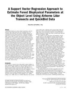
last 110 returns are set as the out-of-sample data, which are used for prediction and evaluation. The average performance of the SVR during the first 500 trading days, that is, from January 4, 2010, to February 1, 2012, is used for determining the kernel parameters. The last 500 trading days, that is, from February 2, 2012, to March 3, 2014, is used for performance comparison against the commonly used kernels. To improve the performance, the logarithmic returns are normalized to [−1, 1] before being input into the SVR. 4.2. Determining the Kernel Parameters. Before evaluating the performance of the new kernel, multiple parameters still need to be determined to make best use of the kernel. The undetermined parameters are 𝑚, which measures how many historical data are used, 𝜆, which measures how fast the impact of one event decays with time, and Δ𝑡, which indicates how we represent 1 minute numerically. We optimize the parameters according to the out-of-sample forecast performance of the corresponding SVR, which is evaluated by MSE and hit rate, respectively. MSE is the mean square error of the predictions and is computed using the normalized returns. Hit rate is the proportion of predicted returns that have the same sign with the actual ones, that is, the directional forecast accuracy rate. To determine 𝑚, all the other parameters are fixed, and 𝑚 varies from 1 to 30. The average MSE and hit rate in the first 500 trading days are plotted in Figures 1(a) and 1(b), respectively. (Figures 1(a) and 1(b) are plotted with 𝜆 and Δ𝑡 set to the optimal values. Actually, the trends of the plots do not vary with the other kernel parameters.) The average MSE decreases sharply with 𝑚 when 𝑚 ≤ 21, is relatively constant when 𝑚 ∈ [21, 26], and decreases slowly with 𝑚 when 𝑚 ∈ [26, 30]. The average hit rate increases sharply with 𝑚 when 𝑚 ≤ 21, is relatively constant when 𝑚 ∈ [21, 25], and gets smaller afterwards. Considering that smaller MSE and greater hit rate are preferred, 𝑚 = 30 and 𝑚 ∈ [21, 25] are all appropriate choices suggested by the experiments. In the following comparative experiments, 𝑚 is set to 25. (We have also done comparative experiments with 𝑚 set to the other suggested values, and the results are consistent.) To determine 𝜆, all the other parameters are fixed, and 𝜆 varies from 1 to 50. The average MSE and hit rate in the first 500 trading days are plotted in Figures 2(a) and 2(b), respectively. It is quite clear that the minimum average MSE and maximum average hit rate are both achieved at 𝜆 = 10, and thus we set 𝜆 to 10 in the following comparative experiments. The same method is used to optimize Δ𝑡, and the average MSE and hit rate are plotted in Figures 3(a) and 3(b), respectively. We can see that the minimum average MSE and maximum average hit rate are both achieved at Δ𝑡 = 0.05, and thus we set Δ𝑡 to 0.05 in the following comparative experiments. 4.3. New Kernel versus Commonly Used Kernels. The new kernel is compared with the commonly used kernels in terms of the out-of-sample forecast performance of the corresponding SVR. Although any function satisfying Mercer’s condition

Mathematical Problems in Engineering

5

0.036

500-day average hit rate

500-day average MSE

0.035 0.034 0.033 0.032

0.72

0.71

0.7

0.031 0.03

0

5

10

15 (m)

20

25

0.69

30

0

5

10

15

20

25

30

(m)

(a) Average MSE versus 𝑚

(b) Average hit rate versus 𝑚

0.037

0.73

0.036

0.72 500-day average hit rate

500-day average MSE

Figure 1: 500-day average MSE and hit rate achieved with different values of 𝑚.

0.035 0.034 0.033 0.032 0.031

0.71 0.7 0.69 0.68

0

10

20

30

40

50

𝜆

(a) Average MSE versus 𝜆

0.67

0

10

20

30

40

50

𝜆

(b) Average hit rate versus 𝜆

Figure 2: 500-day average MSE and hit rate achieved with different values of 𝜆.

can be used as the kernel function, radial basis function and sigmoid function are two widely used kernels. The former tends to outperform others under general smoothness assumption [12], and the latter gives a particular kind of twolayer sigmoidal neural network [15]. Thus, these two kernel functions are used for performance comparison. We realize each SVR by LIBSVM-3.20 [19], and the related codes are modified for the new kernel. The out-of-sample MSE and hit rate are computed for each of the three kernels on each of the last 500 trading days. The results of the new kernel are plotted against those of the radial basis function kernel and the sigmoid function kernel in Figures 4 and 5, respectively. In Figure 4(a), the vertical and horizontal axes represent the MSE of the new kernel and the radial basis function kernel, respectively, while, in Figure 4(b), the vertical and horizontal axes represent the hit rate of the new kernel and the

radial basis function kernel, respectively. There are 500 points corresponding to the 500 trading days plotted in each subplot, and the diagonal line representing 𝑦 = 𝑥 is for reference. We can see that most points lie below the line 𝑦 = 𝑥 in Figure 4(a) and lie above the line 𝑦 = 𝑥 in Figure 4(b). This indicates that the new kernel leads to smaller MSE and greater hit rate than the radial basis function kernel in most of the 500 trading days. Similarly, Figures 5(a) and 5(b) indicate that the new kernel leads to smaller MSE and greater hit rate than the sigmoid function kernel in most of the 500 trading days. Therefore, the SVR with the new kernel has obviously better forecast performance in terms of both the MSE and the hit rate. In addition, a simple trading strategy is carried out based on the out-of-sample forecasts of the SVR with different kernel specifications. The initial capital is set as 100 on each trading day. The index is bought if the one-step-ahead

6

Mathematical Problems in Engineering 0.037

0.73 500-day average hit rate

500-day average MSE

0.036 0.035 0.034 0.033

0.71

0.7

0.032 0.031

0.72

0

20

40

60 Δt(×100)

80

100

0.69

120

0

(a) Average MSE versus Δ𝑡

20

40

60 Δt(×100)

80

100

120

(b) Average hit rate versus Δ𝑡

Figure 3: 500-day average MSE and hit rate achieved with different values of Δ𝑡.

0.14

0.85

0.12 0.75 Hit rate-new kernel

MSE-new kernel

0.1 0.08 0.06 0.04

0.65

0.55

0.45 0.02 0

0

0.02

0.04 0.06 0.08 0.1 MSE-radial basis kernel

0.12

0.14

(a) MSE

0.35 0.35

0.45

0.55 0.65 Hit rate-radial basis kernel

0.75

0.85

(b) Hit rate

Figure 4: New kernel versus radial basis function kernel from February 2, 2012, to March 3, 2014.

predicted return is positive and exceeds a threshold and sold if the one-step-ahead predicted return is negative and below a threshold, and no action is performed otherwise. The threshold is set as the average of the (100 + 𝑚) normalized returns in the training period divided by the scale coefficient of ln(1000). (The scale coefficient controls the trading strategy’s sensitivity to index price change, and a higher value leads to more frequent trading. The value of ln(1000) is arbitrarily set and can be adjusted. The results are consistent as the scale coefficient varies.) The variation of capital under such a strategy in the 110minute out-of-sample period on February 2, 2012, is plotted in Figure 6(a). We can see that the new kernel leads to higher capital gain than the other two kernels most of the time. Also, the average capital variation in the last 500 trading days is plotted in Figure 6(b). Unlike the fluctuant plots in Figure 6(a), the capital increases steadily when it is averaged

over the 500-day period, no matter which kernel is used. This confirms the effectiveness of SVR in forecasting highfrequency stock returns. Once again, the new kernel leads to the highest capital gain and the advantage gets more obvious as the trading period is prolonged. At the end of a day, the new kernel leads to a return at about 0.6%/110 min on average, while the resulting returns of the other two kernels are both less than 0.4%/110 min on average. Furthermore, Student’s 𝑡-test is used to test whether the new kernel significantly outperforms the commonly used kernels. Specifically, we calculate the differences of MSE, hit rate, and 110-minute capital gain between the forecasts with the new kernel and those with each comparative kernel, respectively, on each of the last 500 trading days. Table 1 reports the mean (𝑥𝑑 ) and the standard deviation (𝑠𝑑 ) of these differences in these 500 trading days. We test the null hypothesis that “the forecasts with the new kernel and those

Mathematical Problems in Engineering

7 0.85

0.14 0.12

0.75 Hit rate-new kernel

MSE-new kernel

0.1 0.08 0.06 0.04

0.65

0.55

0.45 0.02 0

0

0.02

0.04

0.06 0.08 0.1 MSE-sigmoid kernel

0.12

0.35 0.35

0.14

0.45

0.55 0.65 Hit rate-sigmoid kernel

(a) MSE

0.75

0.85

(b) Hit rate

Figure 5: New kernel versus sigmoid function kernel from February 2, 2012, to March 3, 2014.

100.6

102.5

100.5

Average capital

102

Capital

101.5

101

100.5

100

100.4 100.3 100.2 100.1 100

0

20

40

60 Time (min)

80

100

120

New kernel Radial basis kernel Sigmoid kernel

0

20

40

60

80

100

120

Time (min) New kernel Radial basis kernel Sigmoid kernel

(a) Capital variation on February 2, 2012

(b) Average capital variation from February 2, 2012, to March 3, 2014

Figure 6: Capital variation of a simple trading strategy.

with the comparative kernel have the same accuracy in terms of the specified criterion,” with the comparative kernel and the criterion specified in the first row and the second row of Table 1, respectively. The 𝑡-statistics are reported in the last row of Table 1. We can easily see that the six null hypotheses are all significantly rejected. The new kernel has smaller MSE, greater hit rate, and higher 110-minute capital gain than both the radial basis function kernel and the sigmoid function kernel. And the differences are all significant at the 1% level. Therefore, the results of Student’s 𝑡-test indicate that the improvement in out-of-sample forecast accuracy brought about by the new kernel is significant both statistically and economically, and

thus the new kernel is preferred in forecasting high-frequency stock returns.

5. Summary and Conclusion Support vector machine for regression is now widely applied in time series forecasting problems. Commonly used kernels such as the radial basis function kernel and the sigmoid function kernel are first derived mathematically for pattern recognition problems. Although their direct applications in time series forecasting problems can generate remarkable performance, we argue that using a kernel designed according

8

Mathematical Problems in Engineering Table 1: Out-of-sample forecast performance comparison results from February 2, 2012, to March 3, 2014 (𝑛 = 500).

Criterion 𝑥𝑑 𝑠𝑑 𝑡=

𝑥𝑑 √𝑛 𝑠𝑑

New kernel versus (minus) radial basis kernel MSE Hit rate 110-min gain −1.5201𝑒 − 3 4.8709𝑒 − 2 2.0250𝑒 − 3 5.3684𝑒 − 3 6.0785𝑒 − 2 2.8530𝑒 − 3 −6.33∗∗∗

17.92∗∗∗

15.87∗∗∗

New kernel versus (minus) sigmoid kernel MSE Hit rate 110 min gain −1.3917𝑒 − 3 5.3945𝑒 − 2 2.3879𝑒 − 3 5.3658𝑒 − 3 6.3875𝑒 − 2 3.2202𝑒 − 3 −5.80∗∗∗

18.88∗∗∗

16.58∗∗∗

Note: ∗∗∗ indicates significance at the 1% level.

to the specific nonlinear dynamics of the series under study can further improve the forecast accuracy. Under the assumption that each high-frequency stock return is an event that triggers momentum and reversal periodically, we decompose each future return into a collection of decaying cosine waves that are functions of past returns. Under realistic assumptions, we reach an analytical expression of the nonlinear relationship between past and future returns and thus design a new kernel specifically for forecasting high-frequency stock returns. Using highfrequency prices of Chinese CSI 300 index as empirical data, we determine the optimal parameters of the new kernel and then compare the new kernel with the radial basis function kernel and the sigmoid function kernel in terms of the SVR’s out-of-sample forecast accuracy. It turns out that the new kernel significantly outperforms the other two kernels in terms of the MSE, the hit rate, and the capital gain from a simple trading strategy. Our empirical experiments confirm that it is statistically and economically valuable to design a new kernel of SVR specifically characterizing the nonlinear dynamics of the time series under study. Thus, our results shed light on an alternative direction for improving the performance of SVR. Current study only utilizes past returns to predict future returns. A natural extension is to introduce intraday trading volumes and intraday high/low prices into the feature vector of the SVR and develop kernels characterizing the corresponding nonlinear relationship between future return and feature vector. Another possible extension is to apply the SVR with new kernel in the energy markets where trading is continuous 24 hours. We leave them for future work.

Competing Interests The authors declare that they have no competing interests.

Acknowledgments The authors are grateful for the financial support offered by the National Natural Science Foundation of China (71201075) and the Specialized Research Fund for the Doctoral Program of Higher Education of China (20120091120003).

References [1] D. A. Hsieh, “Testing for nonlinear dependence in daily foreign exchange rates,” The Journal of Business, vol. 62, no. 3, pp. 339– 368, 1989.

[2] J. A. Scheinkman and B. LeBaron, “Nonlinear dynamics and stock returns,” The Journal of Business, vol. 62, no. 3, pp. 311–337, 1989. [3] G. S. Atsalakis and K. P. Valavanis, “Surveying stock market forecasting techniques-part II: soft computing methods,” Expert Systems with Applications, vol. 36, no. 3, pp. 5932–5941, 2009. [4] V. N. Vapnik, The Nature Of Statistical Learning Theory, Springer, New York, NY, USA, 1995. [5] L. Cao and F. E. H. Tay, “Financial forecasting using support vector machines,” Neural Computing & Applications, vol. 10, no. 2, pp. 184–192, 2001. [6] L. J. Cao and F. E. H. Tay, “Support vector machine with adaptive parameters in financial time series forecasting,” IEEE Transactions on Neural Networks, vol. 14, no. 6, pp. 1506–1518, 2003. [7] K.-J. Kim, “Financial time series forecasting using support vector machines,” Neurocomputing, vol. 55, no. 1-2, pp. 307–319, 2003. [8] V. V. Gavrishchaka and S. Banerjee, “Support vector machine as an efficient framework for stock market volatility forecasting,” Computational Management Science, vol. 3, no. 2, pp. 147–160, 2006. [9] S. Sonnenburg, G. R¨atsch, C. Sch¨afer, and B. Sch¨olkopf, “Large scale multiple kernel learning,” Journal of Machine Learning Research, vol. 7, pp. 1531–1565, 2006. [10] A. Rakotomamonjy, F. R. Bach, S. Canu, and Y. Grandvalet, “Simple MKL,” Journal of Machine Learning Research, vol. 9, pp. 2491–2521, 2008. [11] C.-Y. Yeh, C.-W. Huang, and S.-J. Lee, “A multiple-kernel support vector regression approach for stock market price forecasting,” Expert Systems with Applications, vol. 38, no. 3, pp. 2177–2186, 2011. [12] W. Huang, Y. Nakamori, and S.-Y. Wang, “Forecasting stock market movement direction with support vector machine,” Computers and Operations Research, vol. 32, no. 10, pp. 2513– 2522, 2005. [13] J. M. Mat´ıas and J. C. Reboredo, “Forecasting performance of nonlinear models for intraday stock returns,” Journal of Forecasting, vol. 31, no. 2, pp. 172–188, 2012. [14] J. C. Reboredo, J. M. Mat´ıas, and R. Garcia-Rubio, “Nonlinearity in forecasting of high-frequency stock returns,” Computational Economics, vol. 40, no. 3, pp. 245–264, 2012. [15] C. J. C. Burges, “A tutorial on support vector machines for pattern recognition,” Data Mining and Knowledge Discovery, vol. 2, no. 2, pp. 121–167, 1998. [16] J. C. Platt, “Fast training of support vector machines using sequential minimal optimization,” in Advances in Kernel Methods: Support Vector Learning, B. Sch¨olkopf, C. J. C. Burges, and A. J. Smola, Eds., chapter 12, pp. 185–208, MIT Press, Cambridge, Mass, USA, 1999.

Mathematical Problems in Engineering [17] T. Chordia, R. Roll, and A. Subrahmanyam, “Evidence on the speed of convergence to market efficiency,” Journal of Financial Economics, vol. 76, no. 2, pp. 271–292, 2005. [18] D. Y. Chung and K. Hrazdil, “Speed of convergence to market efficiency: the role of ECNs,” Journal of Empirical Finance, vol. 19, no. 5, pp. 702–720, 2012. [19] C. W. Hsu, C. C. Chang, and C. J. Lin, “A practical guide to support vector classification,” Tech. Rep., Department of Computer Science, National Taiwan University, 2003.

9

Advances in

Operations Research Hindawi Publishing Corporation http://www.hindawi.com

Volume 2014

Advances in

Decision Sciences Hindawi Publishing Corporation http://www.hindawi.com

Volume 2014

Journal of

Applied Mathematics

Algebra

Hindawi Publishing Corporation http://www.hindawi.com

Hindawi Publishing Corporation http://www.hindawi.com

Volume 2014

Journal of

Probability and Statistics Volume 2014

The Scientific World Journal Hindawi Publishing Corporation http://www.hindawi.com

Hindawi Publishing Corporation http://www.hindawi.com

Volume 2014

International Journal of

Differential Equations Hindawi Publishing Corporation http://www.hindawi.com

Volume 2014

Volume 2014

Submit your manuscripts at http://www.hindawi.com International Journal of

Advances in

Combinatorics Hindawi Publishing Corporation http://www.hindawi.com

Mathematical Physics Hindawi Publishing Corporation http://www.hindawi.com

Volume 2014

Journal of

Complex Analysis Hindawi Publishing Corporation http://www.hindawi.com

Volume 2014

International Journal of Mathematics and Mathematical Sciences

Mathematical Problems in Engineering

Journal of

Mathematics Hindawi Publishing Corporation http://www.hindawi.com

Volume 2014

Hindawi Publishing Corporation http://www.hindawi.com

Volume 2014

Volume 2014

Hindawi Publishing Corporation http://www.hindawi.com

Volume 2014

Discrete Mathematics

Journal of

Volume 2014

Hindawi Publishing Corporation http://www.hindawi.com

Discrete Dynamics in Nature and Society

Journal of

Function Spaces Hindawi Publishing Corporation http://www.hindawi.com

Abstract and Applied Analysis

Volume 2014

Hindawi Publishing Corporation http://www.hindawi.com

Volume 2014

Hindawi Publishing Corporation http://www.hindawi.com

Volume 2014

International Journal of

Journal of

Stochastic Analysis

Optimization

Hindawi Publishing Corporation http://www.hindawi.com

Hindawi Publishing Corporation http://www.hindawi.com

Volume 2014

Volume 2014