A New Statistical Model for Site-Specific Indoor Radio ... - CiteSeerX

112

IEEE TRANSACTIONS ON WIRELESS COMMUNICATIONS, VOL. 1, NO. 1, JANUARY 2002

A New Statistical Model for Site-Specific Indoor Radio Propagation Prediction Based on Geometric Optics and Geometric Probability Mudhafar Hassan-Ali, Member, IEEE and Kaveh Pahlavan, Fellow, IEEE

Abstract—The ray-tracing (RT) algorithm has been used for accurately predicting the site-specific radio propagation characteristics, in spite of its computational intensity. Statistical models, on the other hand, offers computational simplicity but low accuracy. In this paper, a new model is proposed for predicting the indoor radio propagation to achieve computational simplicity over the RT method and better accuracy than the statistical models. The new model is based on the statistical derivation of the ray-tracing operation, whose results are a number of paths between the transmitter and receiver, each path comprises a number of rays. The pattern and length of the rays in these paths are related to statistical parameters of the site-specific features of indoor environment, such as the floor plan geometry. A key equation is derived to relate the average path power to the site-specific parameters, which are: 1) mean free distance; 2) transmission coefficient; and 3) reflection coefficient. The equation of the average path power is then used to predict the received power in a typical indoor environment. To evaluate the accuracy of the new model in predicting the received power in a typical indoor environment, a comparison with RT results and with measurement data shows an error bound of less than 5 dB. Index Terms—Power coverage, power delay profile, probabilistic geometry, rat tracing, site-specific channel model, statistical indoor radio propagation, wireless deployment tool.

I. INTRODUCTION

W

E ARE living with ever increasing demand on telecommunications speed and ubiquity. The advent of the Internet and data networks has escalated this demand. The mobility and ease of installation make wireless communication networks one of the most important communication systems to deploy. Personal communications systems (PCS), wireless local area networks (WLANs), wireless private branch exchanger (WPBXs), and Home Phoneline Network Alliance (HomePNA) are the services that are being deployed in indoor areas on an increasing scale. The latter application is proving to have a large market since it will be integrated to the emerging Digital Subscriber Loop technologies (ADSL, VDSL, etc.). The market of these services will try to reach out to offices, schools, hospitals, and factories [10], [12]. Because the indoor radio Manuscript received December 1, 1999; revised February 1, 2001; accepted March 7, 2001. The editor coordinating the review of this paper and approving it for publication is R. Valenzuela. M. Hassan-Ali is with the Systems Engineering, Alcatel USA, Petaluma, CA 94954 USA. K. Pahlavan is with the CWINS, Worcester Polytechnic Institute, MA 01609 USA. Publisher Item Identifier S 1536-1276(02)00185-X.

channel has a tremendous amount of impairment and variability [1], [5], [6], large-scale deployment of these services provides a major challenge to the network designers. For this reason, it is imperative to develop deployment tools, where efficient but accurate radio channel models are required. The efficiency of a model is measured by the computational complexity, whereas accuracy is measured by the estimation error. Ray-tracing (RT) [1], [14], [20] is one of the most popular techniques for predicting radio channels used in the deployment tools. The main characteristic of the RT is the computational intensity, which is the main reason for the prediction tools to be slow in spite of its accuracy compared to the tools based on the statistical model. This has motivated a significant research effort to pursue alternative methods including the so-called Fast RT [2], [21] in an attempt to expedite the computation time. Still these alternative methods require more complex floor-plan databases and the need to trace all rays regards of their significance to the received power. The purpose of this paper is to introduce a new model for statistically predicting the indoor radio propagation in order to contrive a more computationally efficient method for predicting the received power within a building. The paper is organized as follows. Section II states the theory behind the new model and presents a key equation for estimating path power. Section III shows a method whereby the total received power can be estimated. In Section IV, the prediction of indoor radio power using the new model is compared to the prediction of RT software and data collected from measurements for a typical office environment. II. POWER OF A PATH WITH A GIVEN LENGTH RT approximates the radio propagation in a finite number of rays originated from the transmitter. Each ray encounters reflection and transmission upon intersecting with an obstacle (such as walls, doors, windows, etc.) The pattern of ray propagation is dictated by the geometry of the floor layout and the materials from which these obstacles are made. Hence, as an alternative, the statistical characterization of radio propagation can be related explicitly to the statistics of these patterns [4]. The statistical features of the propagation can be deduced directly from the layout and the materials of the floor under consideration. The purpose of this section is to relate the path power to the key site-specific propagation parameters. The path power relationship will be used in Section III to predict the received power.

1536–1276/02$17.00 © 2002 IEEE

HASSAN-ALI AND PAHLAVAN: STATISTICAL MODEL FOR SITE-SPECIFIC INDOOR RADIO PROPAGATION PREDICTION

113

A. Path Power and the Number of Reflections and Transmissions When a path arrives at a point, it has already gone through many reflections and transmissions (object-intersections). Consequently, the path power tends to decay rapidly with distance more than the inverse-square distance law for the free-space. Each path is traced throughout its entire trip from the transmitter to the receiver. Each time there is an object-intersection the ray loses a certain amount of power while the propagation loss in between intersections will maintain the free-space rate, i.e., inverse-square distance law. The intersection loss is either due to reflection or transmission, since other mechanism, such as diffraction and diffused scatter, can be ignored in indoor propagation [9]. Each loss can be expressed in power formulation as a multiplication by a loss coefficient. Hence, after traveling meters from the transmitter (Tx) and undergoing intersections transmissions), the path power is ex( reflections and pressed (1) where and are the mean “voltage” reflection and transmisis the free-space power at dission coefficients, respectively, tance 1 meter, which is expressed by

Where and ( for isotropic antenna) are gain of is the speed transmit and receive antennas, respectively, of light in free space, and is the frequency of the radio signal, which is 900 MHz in this paper. For rest of this paper, the assumption is that the transmit and receive antennas are isotropic; i.e., omni-directional propagation. The mean path power can be expressed as follows:

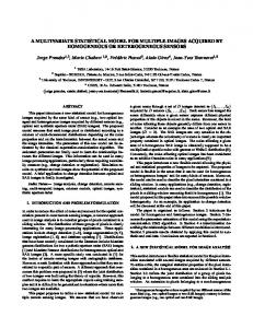
Fig. 1.

The rectangular model used to find PDF of q and p.

is the mean free distance between two intersections, where which depends on the floor layout Mean Free Distance. It is defined as the mean distance a ray can travel before it intersects with an object. This parameter is estimated within a given shape, which is assumed to be rectangular due to the adoption of the rectilinear model. In Section III-C, a method for estimating this parameter will be presented using probabilistic techniques. The from knowing the width and length of the method estimates , rectangles of the floor plans. The second function on the other hand, gives the probability of having exactly reflections and transmissions in path length . As mentioned earlier, these are independent and exclusive, hence binomial PDF fits these conditions [18]. Then

(2) (5) is the PDF of a path that intersects objects where transafter traveling distance with reflections and missions. In the following section, this PDF will be discussed in detail.

and are the probabilities of reflection and transwhere mission, respectively, for a path of length . Note that . After a few manipulations on (2) we obtain the following results (see Appendix A for derivation):

B. Calculation of

(6)

One can think of the process of hitting obstacles as a combination of reflections and transmissions. These two events are independent and exclusive in one path at one instance. Hence, can be decomposed as a multiplication of two functions (3) is the PDF for a path that has undergone inwhere tersections after traveling distance . In [13], it has been demonstrated through a Monte Carlo simulation that this function is a Poisson distribution for the indoor environment. Hence (4)

This equation gives an explicit relationship between the average power of a path with site-specific details and the building layout via , and the floor materials via ( and ). By estimating the values of these parameters based on the location of both transmitter and receiver, (6) can be applied to predict the power of a path versus distance. C. Calculation of

and

To use (6) for predicting the power of a multipath arrival knowing the location of the transmitter and the receiver, it is important to know how and change with path distance . In order to do that, let denote the Transmitter–Receiver distance, therefore, , where is the difference between

114

Fig. 2.


The probability distribution of reflection (p).

the total path length and Transmitter–Receiver distance. Hence , because LOS can not undergo any reflections. For large excess path lengths, reflection and transmission events are taken to be equally likely; i.e., approaches 0.5. Therefore, one can conjecture that this behavior can be exponential, i.e.,

D. General Formula for Path Power Substituting (7) in (6) yields (8) Note serves as the time delay of the profile since where is the speed of light. Hence

,

(7) A Monte Carlo simulation has supported this conjecture where the rectangular shape model is employed. The simulation can be summarized as follows: The rectangular model of a floor plan is taken to be 10 5 with 50% uniform randomness in both where length and width. This means that the width is is a uniform random variable in the range of , where is a uniform random variable and the length is . A numerous number of rays that have in the range of undergone through intersections are generated. For each ray, the type of intersection (reflection or transmission) is recorded at each intersection as seen in Fig. 1. The reach and length of each path are then computed, where the reach of a path is the direct distance between Tx and Rx , while the path is equivalent to . Hence, and are is estimated. assigned for each from which the PDF of Fig. 2 shows the result of this simulation. In this figure, both the PDF’s derived from simulation and the best exponential fit estimated is very close are plotted together. The value of to the “mean free distance” of a rectangle with the dimension of 10 5 as can be calculated using the formulas presented in Section III-C.

(9) This equation represents an “average” power delay profile for indoor radio channel. To visualize the significance of the parameters to the shape of the profile, Fig. 3(a)–(d) show profiles where one parameter is made variable while the others are held constant. The most influential parameter is the Tx–Rx distance, whereas ranks second. and have a roughly similar effect. , then (9) will give the expected value of Note that when the power for the LOS ray (10) Clearly, LOS power is inversely proportional to squared Tx–Rx distance (free-space component), and exponentially is the to transmission loss in this distance. Note that average transmission loss (no Reflection coefficient exists is the mean number of transmission since it is LOS), and occurrences within . Since the LOS ray is nothing more than the line drawn between Tx and Rx, this portion of signal power can be replace by the deterministic power calculation. If there


Fig. 3.

115

The model parameters and their effect of predicted channel profiles.

are object-intersections along this line, then the correction to (8) and, therefore, to (9) will be as

No close form could be found for this integral, thus, it has to be computed numerically as (12b)

(11)

III. THE MULTIPATH RECEIVED POWER In this section, the total power received from multiple paths will be estimated based on the key equation derived in the previous section. For a wideband receiver, the multipath power is simply defined as the sum of the their individual power regardless of the phase of the individual paths [19]; i.e., (12a)

where is the bin time unit. In (12b), it is assumed that a path exists in each bin, which is 5 ns in this case, since the bandwidth is 200 MHz. The result from (12b) will be compared to the power estimation using RT results as well as measurement data. In the following two subsections, methods for determining the three parameters ( , , and ) are presented. A. The Area Where

,

and

to be Estimated

For a given pair of (Tx, Rx), we need to identify the neighborhood; i.e., obstacles surrounding Tx and Rx, that influences the estimation of the received power by determining the mean value of , , and . To identify these obstacles, maximum path

116


length can serve as an indication of how far the inclusion of the obstacles should be. The path power is assumed to reach a threshold (say 10 dB below the strongest ray arrives at Rx) under which the ray will be neglected. The shape of area that the maximum path length traverses before its power drops below the threshold is naturally ellipsoid. Within this ellipsoid shape, the path is expected to have the lowest power when it undergoes only one reflection out of intersections. This is true on a statistical basis, since in (assuming that ). general As depicted in Fig. 4, the locations of Tx and Rx serve as the foci of the ellipse whose boundary acts as the farthest reflector on which rays bounce with the same length. The idea of confining the area of interest inside an ellipsoid shape has been presented in the literature primarily for studying the mulitpath scattering [15]. Rectilinear partitioning of the floor plan simplifies the issue of deciding which spaces that the ellipse overlaps have to be included in the estimation of the three model parameters. During rectilinear partitioning process, fictitious exten(no transmission loss) sions will be drawn and assigned (no reflection). These extensions will be included and a during the estimation of the average model parameters ( and ), see Fig. 4. If the maximum path length is denoted by , then the threshold is computed as (13a) where is the maximum power of a ray that travels from dB, Tx to Rx, which can be derived from (8). For then . One method for determining is to use the following equations: for LOS and for OLOS, where is the distance between Rx are deand Tx as seen in Fig. 4. These two equations for rived from numerous evaluations of (8) for various values of its parameters. Another alternative is to use the ad hoc model derived from measurements for the received power; such as JTC, or wall-dependent [1], as follows: (13b) where the decay parameters [1]. B. Estimation of

Fig. 4. An illustrative example for maximum path length relative to the ellipsoid shape.

floor layout.) and expressions [1]:

can be calculated through the following

Horizontal polarization Vertical polarization (15a) (15b) where is the complex permittivity, is the relative normalized dielectric constant, is the conductivity, and is a coefficient that accounts for the transmission loss and it is usually taken to be 0.5 [9]. Note that (15a) is a function of incidence angle; which is a uniform random variable . Therefore, for a given material, one can find the over mean value of the reflection and transmission coefficient by av, i.e., and eraging (15) over .

and

Once the ellipsoid shape is determined, the reflection and transmission coefficients for all objects (say objects) enclosed in it will be collected. Then and are estimated as follows: and

(14)

C. Estimation of The same shape used in the previous section will be used to estimate . In order to estimate the mean value of a random variable , the probability distribution function (PDF) of the ray length is required. Appendix B shows the geometric probability distributions of a ray within the rectangular shape, which was shown to have three different types of rays. The mean free path can be estimated as follows: (16)

are reflection, transmission, and size cowhere , , and efficients, respectively, for object . In a two-dimensional (2-D) case, is the length of the object (such as wall length in the

where , , and denote the mean length of rays between adjacent sides (four cases), opposite width sides, and opposite


117

in proportional to its area overlapping with the ellipse, as indicated in Fig. 4. Hence [16] (18) where is the overlapping area of rectangle , whose area . The assumption is that the ellipse confines is complete rectangles. A part from the having only rectangular shapes, there could be, within the confining ellipse, parallel lines along or axis, such as a portion of a hallway. In this case, the or , mean free distance is computed as respectively. IV. VALIDITY OF THE PROPOSED PREDICTION MODEL In this section, the results of power prediction using the new model are compared to the power predicted by the RT software and the measured power in a typical office environment. The second and the third floors in Atwater Kent (AK2 and AK3, respectively) Laboratories are taken as case study to check the validity of the new model. Throughout this work, we maintained the following parameters for both cases (AK2 and AK3) [7], [8]. • The center frequency of the channel is 1 GHz, and the bandwidth of 200 MHz. • The number of profiles is 620 taken from different locations in the second floor at the AK Labs building. A. Comparison With the Results of RT

Fig. 5.

AK3 floor layout.

length side. They are computed, with assistance of Appendix II, as follows:

(17a)

(17b)

(17c) is comFor rectangle in the floor, a mean free distance and width . Any rectangle inputed based on its length cluded inside the ellipse will be used to estimate the mean value

In this section, the results of the previous subsections will be used for estimating the power in AK3 and then compared with the results obtained from the RT software. In order to do that, the three zones LOS, OLOS1, and OLOS2 are treated individually. On this floor, walls, doors, and windows are considered to be highly dielectric materials, nearly perfect conductors, and low dielectric materials, respectively. Walls are assumed to have a 10 dielectric constant and a 0.001 conductivity, therefore, and coefficients are (0.75,0.48), which are the average over the incidence angle range of . These coefficients are assumed to be (0.95,0.01) and (0.1,0.9) for doors and windows, respectively [3]. 1) LOS: In this case, all Rx’s are located in the same room (number 317) where Tx is as seen in Fig. 5. This room is about m . The distance between Tx and each Rx is in the range from 0.2 to 6 m implying the ellipse for each Tx–Rx combination embracing this room as seen in Fig. 5 and portion of the surrounding hallway (OLOS1) and Room 318. The first step is to estimate and using (14) using the reflection and transmission coefficients given above. The size coefficients are determined for walls as follows: , doors , and windows . Hence, , and . The second step is to estimate from the dimensions of Room 317 and its adjacent vicinities. OLOS1 is a hallway; which is about 2 meters wide. The ellipse only includes about 5 meters of the two parallel walls of OLOS1. Therefore, the dimensions of OLOS1 portion are about m .

118


Notice that in this case equation (17b) or (17c) is used to find . Using (12) in conjunction with (13) yields the estimation of as seen in Table I. 2) OLOS1: Similar analysis can be done for this case. As can be seen in Fig. 5 there are left, right, top, and bottom areas whose parameters are unique because their neighbors are different. The most influential neighbor is Room 317, which possesses about 70% of the ellipse area for this case. Hence is in the range of 0.2 to 0.25 for left, right, and bottom areas. On the other side, the bottom area is shadowed deeply by Room 318. The ellipse in this area embraces parallel walls of Room 318 along the width, with size about 4 3. In this case, is about 0.3 using (17b). The upper boundary of the top area has small rooms (Room 319, Room 320, and the entrance of Room 320-CWINS.) Roughly, their sizes are in the order of 3 2; which cause to be in the range of 0.5 to 0.6. Furthermore, the ellipse does not confine Room 217 entirely, so that is higher than 0.14 as found in LOS. It is estimated to be 0.22 by using (16). Therefore, the average for the top area is in the range 0.4 to 0.6. 3) OLOS2: It consists of a row of offices, most of them of size 3 2 except Rooms 311 and 301. By inspecting Fig. 5, Rooms 301–310 seem to have comparable parameter values. Room 311, on the other hand, is deeply shadowed by Room 318. If we assume that 50% of the ellipse resides inside Room 317, 25% inside LOS1, and 25% inside OLOS2. Then for the Rooms 301–310, is in the range 0.25 to 0.3. Room 312, however, is in a deep shadow due to Room 318. Also, the receivers in this room are the farthest from Tx. The ellipse at the most two adjacent walls (top and right ones) causes to be calculated using (17a) when the two adjacent walls are included. Table II summarizes the parameters that will be used in (11) for all Rx locations in the AK3 experiment to estimate the received power. 4) Results of Power Prediction From the new Model and RT: Fig. 6 shows the scatter plot of power estimated using the new technique versus RT results. The similarity is apparent between the two cases indicating that the new model is a valid technique for power prediction. LOS case shows agreement to all points: i.e., the pattern of power change is very similar. OLOS1 has the same trend except some points located at the intersection of the top with both left and right area of this zone. In the case of OLOS2, the periodical decay is not as deep as the RT results. This is due to the fact that parameter is assumed equal throughout Rooms 301–310. The reality is that the Rooms 308–310 should have a gradual increase to this parameter to account for the gradual increase in the effect of Room 318 shadow. Generally, however, the standard deviation of the prediction with respect to RT estimation is about 5 dB over all zones. However, the standard deviation for the individual zone is as follows: 1.2 dB in LOS, 5.9 dB in OLOS1, 5.5 dB in OLOS2. This is a remarkable achievement considering the fact that the piecewise-linear statistical power modeling [1] had a standard deviation of more than 10 dB. Fig. 7 shows a scatter plot of the predicted power for the three zones. It is apparent that LOS case shows the highest match, whereas results of OLOS-2 show the lowest match.

TABLE I PARAMETER ESTIMATION FOR LOS ZONE

TABLE II MODEL PARAMETERS FOR AK3 IN THREE ZONES

Fig. 6. Power prediction using the new model and RT data versus location index at AK3 (operating frequency is 900 MHz).

When power-distance relationship is drawn with both axes are logarithmic, as seen in Fig. 8, the shape of the relation is anticipated to be slowly decaying approximately in the first 10 meters and the decay becomes much steeper [9], [11] . In [11], empirically this relationship was fit to an exponentially decaying function; i.e., , which is very close to our theoretical derivation as showed in (6).

B. Comparison Between the Results From the New Model and Measurements To compare the prediction of the received power with those obtained from measurements, the frequency-domain measure-


Fig. 7.

119

Comparison of power prediction using the new model and RT data at the three zones of AK3 (operating frequency is 900 MHZ).

Fig. 8. Power prediction using the new model and RT data versus Tx–Rx distance at AK3 (operating frequency is 900 MHz).

ments for AK2 used in [9] will be employed here also. A similar analysis is carried out to the locations (see Fig. 9) to find the three parameters in each location. The materials of walls, windows, and doors are similar to AK3 floor mention above. The estimation of the three parameters as done in Section IV-A is repeated here, as seen in Table III. Compared to

AK3 floor, the value of is the same, whereas is slightly smaller due to the fact that this floor has more metallic doors. The receivers in Room-1, where the transmitter is located, are associated to the four surrounding spaces according to their closeness to these spaces. The fifth space consists of the receivers in Room-4.

120


TABLE III MODEL PARAMETERS FOR AK2

rectangular shape in the floor plan. This operation is performed once for each floor plan under study. 3) Locate the Transmitter (Tx) and Receiver (Rx) in the floor plan. 4) Draw an ellipse, whose foci are the locations of Tx and Rx as explained in Section III-A. 5) Find the overlapping area between the ellipse and the floor plan. This step identifies the inclusion of all rectangular shapes (rooms) that will be use in the next step. 6) Compute the average values of , , and for the overlapping area identified in the step 5) using(14) and (18). 7) Use the parameters computed in the step 6) in (11) and (12) to estimate the multipath received power.

Fig. 9.

AK3 floor layout.

The result of the power prediction is depicted in Fig. 10. The standard deviation between the prediction and measurement is about 2.87 dB and the mean error is 2.77 dB, compared to a standard deviation of 2.4 dB when using RT [3]. Fig. 11 shows the power levels obtained from three methods; i.e., measurement, RT [8], and the new model at AK2.

V. THE COMPUTATIONAL COMPLEXITY OF THE NEW METHOD COMPARED TO RT According to the new method, the multipath-received power is estimated using the following algorithm. A. Algorithm 1) Perform the rectilinear partitioning (rectangulation) of the floor plan. The result is that the floor plan is partirectangles, where is tioned approximately in to the number of walls. 2) Calculate the propagation parameters ( , , and ) as explained in Sections III-B and C. and represent the avfor each erage over the incidence angle range of wall, door, and window using (12). is computed for each

Note that steps 1) and 2) are considered as preprocessing operations and performed once for the floor plan. Steps 4) and 5) are computationally more involved than the rest of the steps in this algorithm. Specifically, step 5) requires answering the query of knowing the rectangles that the ellipse overlaps in a floor plan. queries for checking the The brute-force method results in overlap with all the rectangles in the floor plan for each Tx–Rx pair. This complexity can be improved by using a spatial data structure [22]–[24] for relating the rectangles in a floor plan with each other. This data structure reduces the query time from to , which is the number of the rectangles that overlap with the ellipse in the floor plan. In practice, is determined by the Tx–Rx distance and the size of the rectangles. The rest of the steps are straightforward and are computationally simple, since computation of , , and is performed only once for each rectangle as indicated in step 2. Furthermore, , and are the , for the average value computed over the angle range rectilinear wall model that is assumed in this paper as explained in Section III-B. There are two methods to implement RT; image technique and ray shooting [23]. The RT tool starts with shooting rays from the transmitter to all direction around. Each ray will be traced under it reaches the receiver after undergoing through wall-intersections ( reflections and transmissions). Upon each intersection, the ray splits into two “child” rays, a reflected ray and a transmitted ray. Hence, the number of operations in the brute force ray shooting RT is proportional to


Fig. 10.

121

Power prediction using the new model and measurement data at AK2 (operating frequency is 900 MHz).

Fig. 11. Comparison between power prediction using measurement data, ray-tracing, and the new model at AK2 (operating frequency is 900 MHz).

for distinct paths and without ray splitting [23]. Using triangulation as a data structure, the ray shooting was expedited such that the query of ray-wall intersec1

M

M

1 factor accounts for that the process is repeated times for each shooting 1) factor accounts for the number of rays angle around the transmitter, (2 due to intersections (each intersection spawns 2 rays), and factor accounts searches to find the ray-wall intersection in the for walls; i.e., we require brute-force tracing.

n

N

0

N

tion can be performed in much less than operations. On the other hand, the brute force implementation of the image technique results in a computational complexity proportional to [23]. Beam tracing [24], which is a variation of image technique, is reported recently to have a complexity proportional to . In practice, the parameters and are usually assumed to be 180 and 3, respectively. These parameters, for each Tx–Rx pair, will entail 2700 rays, each one requires power cal-

122


culation at the intersection with a wall. The new model, however, requires a number of computations [using (14) and (18)] equivalent to the number of the rectangles that overlap with the ellipse. In the two floor plans (AK2 and AK3) that this study is based on, the total number of rectangles is less than 50; which implies that the computation ratio is better than 2700 : 50. Furthermore, the new method predicts the average received power, thus, the prediction is less sensitive to the sampling artifact [24] compared to the RT method. We expect that the new model can be useful in optimal placement tools [2]. Fig. 12.

VI. CONCLUSION In this paper, a new model for indoor radio channels is presented. The model relies on the geometric probability of the layout of the indoor environment from which a simple equation for power delay profile was derived. This equation has three key parameters, which are directly related to the geometry of the floor layout and the materials of its walls, doors, and windows through simple equations. The model was, then, used to predict the power received in two office floors, AK2 and AK3 at WPI, and compared with the results obtained from running the RT software and measurement data to check the validity of the new model. It was found that the new prediction had an error bound of 5 dB respect to RT and measurement data. This model can be accepted to surrogate the use of the brute-force RT technique for prediction of radio propagation in indoor environment. The advantage will be in terms of computational simplicity when compared to RT. As a future work, this model can be extended further to include diffracted paths, which can be applied to microcellular environment where reflection and diffraction are the dominant propagation mechanisms. Furthermore, the analysis can be extended to three-dimensional geometry, which enables us to predict power coverage in multistory buildings. APPENDIX I Substituting (4) and (5) in (2) yields

(A-1) By taking out all the factors that are not function of gives

and

(A-2) The inner summation of (A-2) is the binomial expansion of simplified as follows:

(A-3)

A rectangle with different rays between two sides.

Substituting this equation in (A-2) yields (A-4) This summation is Taylor expansion of rewritten as follows:

, hence, it can be

(A-5)

APPENDIX II In this appendix, the Geometric Probability of a ray inside a rectangle will be presented. A number of PDF’s will be derived and to be used for estimation of the mean free distance . Traveling inside a rectangle , a ray can be envisaged geometrically as its hypotenuse between two intersection points. Originally, this ray either came from a reflected parent ray (in), or from a transmitted parent ray coming from an side adjacent rectangle, such as . Therefore, a path from Tx to Rx can be decomposed into a set of these consecutively linked rays. From the basic literature of “Geometric Probability” [16]–[18], the probability distribution function of the ray length can be derived. The derivation of the ray length probability distribution is based on the assumption that the two terminal points of a ray are independent random variables (RV). Moreover, the coordinates of any point in a rectangle have a uniform PDF with respect to length and width of that rectangle [16]–[18]. Fig. 12 are typshows the possible types of rays, i.e., , , and ical examples for these rays. The probability density of the ray is split into three cases. length 1) Rays between adjacent walls, , , , and in Fig. 12: In this case the ray length is expressed as , note that , and . Then the probability distributions is expressed as [16], [17]

(B.1)


2) Rays between opposite sides (width case), In this case, the ray distance is and has a PDF as follows:

3) Rays between opposite sides (length case), This case, the ray distance is and has a PDF as follows:

in Fig. 12:

(B.2) in Fig. 12.

(B.3) After knowing all the possible types of rays in a rectangle, the PDF of the length of a ray irrespective to its relation to the rectangle sides is determined. The probability of having a specific ray type for rays between adja, whereas for rays between opcent sides is . posite sides (either case) the probability is Hence, the PDF of ray length is

(B.4)

ACKNOWLEDGMENT

123

[9] H. Bertoni, W. Honcharenko, L. R. Maciel, and H. Xia, “UHF propagation prediction for wireless personal communications,” Proc. IEEE, vol. 82, pp. 1333–1359, Sept. 1994. [10] J. Keenan and A. Motley, “Radio coverage in buildings,” Br. Telecom Technol. J., vol. 8, pp. 19–24, Jan. 1990. [11] D. Devasirvatham, C. Banerjee, M. Krain, and D. Rappaport, “Multifrequency radiowave propagation measurements in the portable radio environment,” in Proc. IEEE ICC’90, 1990, pp. 1334–1340. [12] D. Molkdar, “Review on radio propagation into and within buildings,” Proc. Inst. Elect. Eng.-H, vol. 138, pp. 61–73, Feb. 1991. [13] M. Hassan-Ali, “Using Ray-Tracing Techniques in Site-Specific Statistical Modeling of Indoor Radio Channels,” Ph.D. dissertation, Worcester Polytechnic Institute, Worcester, MA, 1998. [14] M. Hassan-Ali and K. Pahlavan, “Site-specific wideband and narrowband modeling of indoor radio channel using ray-tracing,” in PMIRC’98, Boston, MA, Sept. 8–11, 1998. [15] R. Ertel, P. Cardieri, K. Sowerby, T. Rappaport, and J. Reed, “Overview of spatial channel models for antenna array communication systems,” IEEE Pers. Commun., vol. 5, pp. 10–22, Feb. 1998. [16] L. Santalo, Integral Geometry and Geometric Probability. Reading, MA: Addison-Wesley, 1976. [17] B. Ghosh, “Random distances within a rectangle and between two rectangles,” Bull. Calcutta Math. Soc., vol. 43, pp. 17–24, 1951. [18] A. Sveshnikov, Problems in Probability Theory, Mathematical Statistics and Theory of Random Functions. New York: Dover, 1968. [19] R. Valenzuela, O. Landron, and D. Jacob, “Estimating local mean signal strength of indoor multipath propagation,” IEEE Trans. Veh. Technol., vol. 46, pp. 203–212, Feb. 1997. [20] J. McKown and R. Hamilton, “Ray tracing as a design tool for radio networks,” IEEE Network Mag., pp. 27–30, Nov. 1991. [21] D. Ullmo and H. Baranger, “Wireless propagation in buildings: A statistical scattering approach,” IEEE Trans. Veh. Technol., vol. 48, pp. 947–955, May 1999. [22] J. O’Rourke, Computational Geometry in C. Cambridge, U.K.: Cambridge Univ. Press, 1993. [23] S. Fortune, “A beam-tracing algorithm for prediction of indoor radio propagation,” in Proc. First ACM Workshop on Applied Computational Geometry, 1996, pp. 76–81. , “Algorithms for the Prediction of Indoor Radio Propagation,”, [24] http://cm.bell-labs.com/cm/cs/who/sjf/pubs.html, 1998.

The authors wish to thank Dr. J. Beneat and Mr. R. Tingley for reviewing the paper and their valuable remarks. Many thanks go to the IEEE JSAC’s reviewers for the constructive comments.

REFERENCES [1] K. Pahlavan and A. Levesque, Wireless Information Networks. New York: Wiley, 1995. [2] S. Fortune, D. Gay, B. Kernighan, O. Landron, R. Valenzuela, and M. Wright, “WISE design of indoor wireless systems: Practical computation and optimization,” IEEE Comput. Sci. Eng., vol. 2, pp. 58–69, Spring 1995. [3] G. Yang, “Performance evaluation of high speed wireless data systems using a 3D ray tracing algorithm,” Ph.D. dissertation, Worcester Polytechnic Inst., Worcester, MA, 1994. [4] P. Bello, “A troposcatter channel model,” IEEE Trans. Commun. Technol., vol. COM-17, pp. 130–137, Apr. 1969. [5] A. Saleh and R. Valenzuela, “A statistical model for indoor multipath propagation,” IEEE J. Select. Areas Commun., vol. SAC-5, pp. 128–137, Feb. 1987. [6] G. Yang, K. Pahlavan, and J. F. Lee, “A 3D propagation model with ploarization characteristics in indoor radio channels,” in Proc. IEEE Globcom, 1993, pp. 1252–1256. [7] R. Ganesh, “Time domain measurements modeling and simulation of the indoor radio channel,” Ph.D. dissertation, Elect. Eng. Dept., Worcester Polytechnic Inst., Worcester, MA, 1991. [8] S. Howard, “Frequency domain characteristics and autoregressive modeling of the indoor radio channel,” Ph.D. dissertation, Elect. Eng. Dept., Worcester Polytechnic Inst., Worcester, MA, 1991.

Mudhafar Hassan-Ali (M’99) was born in Baquba, Iraq, in 1962. He received the B.Sc. and M.S.c. degrees in electrical engineering from University of Baghdad (with highest honors), Bagdad, Iraq, in 1984 and 1989, respectively, and the Ph.D. degree in electrical engineering from Worcester Polytechnic Institute (WPI), Worcester, MA, in 1998. From 1984 to 1987, he was a teaching and research assistant at University Baghdad. From 1989 to 1991, he was an instructor at University of Baghdad, teaching in Electrical Engineering and Computer Science Departments. From 1992 to 1993 he was a lecturer and head of Electronics Engineering Department, University of Seven of April, Libya, From 1993 to 1996, he was with WPI, Electrical Engineering Department and CWINS, where he was involved in Radio Propagation for wireless system design research. In 1996, he joined the Wireline Access System of Alcatel USA, where at present he is a Senior System Architect and has been involved in developing Broadband system access systems based on SONET, xDSL, and IP/ATM technologies. Currently he is leading the effort in building a novel ATM switch fabric for the next generation access system. His Interests are in Communications protocols, VLSI, system architecture, and wireless design. Dr. Hassan-Ali is a member of Eta Kappa Nu and Sigma Xi.

124


Kaveh Pahlavan (M’79–SM’88–F’96) is a Professor of ECE, a Professor of CS, and Director of the Center for Wireless Information Network Studies, Worcester Polytechnic Intitute, Worcester, MA. He is also a Visiting Professor of Telecommunication Laboratory and CWC, University of Oulu, Finland. His area of research is broadband wireless indoor networks. He has contributed to numerous seminal technical publications in this field. He is the principal author of Wireless Information Networks (New York: Wiley, 1995). He has been a consultant to a number companies including CNR, Inc, GTE Laboratories, Steinbrecher Corp., Simplex, Mercurry Computers, WINDATA , SieraComm, 3COM, and Codex/Motorola in Massachusetts; JPL, Savi Technologies, RadioLAN in California, Airnoet in Ohio, United Technology Research Center in Connecticut, Honeywell in Arizona; Nokia, LK-Products, Elektrobit, TEKES, and Finnish Academy in Finland, and NTT in Japan. Before joining WPI, he was the director of advanced development at Infinite Inc., Andover, MA, working on data communications. He started his career as an Assistant Professor at Northeastern University, Boston, MA. He is the Editor-in-Chief of the International Journal on Wireless Information Networks. He was the founder, the program chairman and organizer of the IEEE Wireless LAN Workshop, Worcester, MA, in 1991 and 1996, and the organizer and technical program chairman of the IEEE International Symposium on Personal, Indoor, and Mobile Radio Communications, Boston, MA, in 1992 and 1998. He has also been selected as a member of the Committee on Evolution of Untethered Communication, U.S. National Research Council in 1997, and has lead the U.S. review team for the Finnish R&D Programs in Electronic and Telecommunication in 1999. For his contributions to the wireless networks he was the Westin Hadden Professor of Electrical and Computer Engineering at WPI during 1993–1996, became a fellow of Nokia in 1999. From May of December of 2000, he was the first Fulbright-Nokia scholar at the University of Oulu, Finland. Because of his inspiring visionary publications and his international conference activities for the growth of the wireless LAN industry, he is referred to as one of the founding fathers of the wireless LAN industry. Details of his contributions to this field are available at http://www.cwins.wpi.edu.