for Spike Sorting Using Optimal Quantization. Mingzhou Song and Ha Lam. Department of Computer Science, Queens College, CUNY, Flushing, NY 11367.
A Non-parametric Bayesian Framework for Spike Sorting Using Optimal Quantization Mingzhou Song and Ha Lam Department of Computer Science, Queens College, CUNY, Flushing, NY 11367 Abstract: This paper describes an approach that performs spike sorting by a nonparametric density estimation technique under a Bayesian framework. The technique is based on an optimal quantization method. We performed experiments on simulated and real spike signals. The results are comparable with what is reported in the literature. Key Words: Spike sorting, nonparametric density estimation, quantization.
1.
Introduction
When it is active, a neuron fires spiky signals repetitively, called spike, at a frequency of about 10Hz. A needlelike electrode can be used to record spike signals emitted from nearby neurons. The process of identifying spikes from recorded signals and assigning them to some neurons is called spike sorting. Spike sorting is a method neuroscientists use to inspect neuron activities to investigate the neural system including functions of the brain. As signal recording devices become increasingly powerful, automatic software tools for spike sorting become a necessity, due to the large amount of data produced and the cost of manual spike sorting. Spike sorting is an old, but an evolving, problem, due to faster computers and the availability of multi-electrode data. Challenges are posed by the fact that spike signals are subject to environmental noise and interfering spikes from surrounding neurons, and that the shape and amplitude of the spike itself may change to some extent over time. The simplest spike sorting method is by thresholding. Spike sorting techniques previous to 1998 are reviewed in (Lewicki, 1998). More recent work is described in (Sahani, 1999; Hulata, Segev, & Ben-Jacob, 2001; Oweiss & Anderson, 2002; Menne, Folkers, Malian, Maex, & Hofmann, 2002). Most performance analyses of the spike sorting algorithms are qualitative. Although not necessarily accepted uniformly, some quantitative performance indices are reported: The morphological filter reported in (Menne et al., 2002) achieved 80%±4% correct recognition on data from a simulated cortex containing 90 neurons; Authors of (Hulata et al., 2001) obtain nine wavelet bases by analyzing the data manually. Once they perform Supported by a grant from CUNY Institute for Software Design and Development.
wavelet transform on the data, they use some clustering method to detect spikes. They claim to achieve a recognition rate of around 93% and a false alarm rate of 10%. However, they did not evaluate their wavelet method on separate test data. We use optimal quantization as a non-parametric density estimation technique to represent both the uncertainty associated with the spike shapes themselves and also the environmental noise. Our algorithm includes the following an off-line and an online component. The offline training component obtains a compact representation of the prior knowledge about the spike shapes. The online spike sorting component performs detection and sorting on single channel waveform data using the representation obtained off-line. This paper is organized into four sections. In Section 1 we introduce the spike sorting problem, review existing and our approach. In Section 2, we describe the nonparametric Bayesian framework for spike sorting, including a brief introduction to the non-parametric optimal quantization technique to represent prior spike shape knowledge and evidence from the observed signals. In Section 3, we present the spike sorting results obtained on a simulated spike signal and a real spike signal. Finally, in Section 4, we draw the conclusions and point out further work that might be interesting to do on spike sorting.
2.
A Non-parametric Bayesian Framework for Spike Sorting
Let s be the spike shape. We want to detect it from the observed spike signal x with the help of some prior spike shape knowledge. We formulate this problem in a Bayesian framework. Given the observed data x, our goal is to find a spike shape s that maximizes the posteriori probability p(s|x), which is proportional to the product of the probability of the prior probability p(s) of the spike shape s, and the conditional probability p(x|s) of observing the spike signal x given a spike shape s, that is, p(s|x) ∝ p(s) · p(x|s). In the off-line process, p(s) is obtained, and in the online process, p(x|s) is obtained. Both of these processes make use of a non-parametric density estimation technique based on quantization. After p(s|x) is obtained, we can compare this to a probability threshold and then
2.1
A Nonparametric Density Estimation Technique based on Optimal Quantization
A problem in statistical learning is to estimate the probability density function (p.d.f.) from observed data. The classical approach to solving the problem is to assume the p.d.f. comes from a family of parametric forms, such as the p.d.f. of the Gaussian distribution. Then the parameters are estimated from the observed data by, for example, maximum likelihood principle. The family and a set of parameters specify a unique p.d.f. Issues with this parametric approach include that it usually is not clear in advance from which distribution family the observed data may come from. When a family is blindly chosen, large biases may arise from a wrong assumption. One way to reduce the biases is to select a model from multiple families. However, since the families can not describe all possible p.d.f.’s, large biases may still exist. An alternative to the parametric approach is the nonparametric approach, which does not assume any family for the p.d.f. of the population where the observed data were drawn. Thus, the biases can be controlled and minimized. Typical nonparametric techniques include Parzen windows, k-nearest neighbors, splines, and histograms. The first three approaches become extremely computationally intensive in moderately higher dimension. An equal spacing multi-dimensional histogram usually does not guarantee consistency. The nonparametric density estimation approach that we use is based on an optimal quantization of the sample space. We quantize the space using a multi-dimensional non-uniform spacing grid. The grid is obtained by maximizing a quantizer performance measure defined as follows: T (Q) = WJ J(Q) +WH H(Q)
(1)
where Q represents the quantizer, J(Q) is the log likelihood of the observed data, H(Q) is the entropy of the observed data on the grid, WJ is the weight of the log likelihood, and WH is the weight of the entropy. This measure controls the over/under-fitting via the weights WJ and WH . We usually use non-negative values for WJ and WH . Only the ratio of the two weights affect the quantizer. When WJ /WH → ∞, the quantizer behaves towards over-fitting; when WJ /WH → 0, the quantizer behaves towards under-fitting. We first obtain a quantization grid for the observed data by a genetic algorithm. Then a density function is estimated using an approach similar to the k-nearest neighbor smoothing. The smoothing eliminates zero density estimates in cells where there is no observed data.
2.2
Representing Prior Spike Shape Probability
The prior spike shape probability density function, p(s), indicates how often we expect to see a spike shape represented by a vector s. To estimate the probability density function p(s), we first gather groundtruth spikes. Unfortunately, such data are usually not directly available because the labor cost for labeling the spikes from recorded signals is very high. We obtained the groundtruth by setting a very high threshold on the real signals that we have. We consider those signal chunks that cross the threshold to be true spikes. An individual spike lasts about 1 millisecond. Given the sampling frequency in tens of kilo-Hertz, a discretized spike contains hundreds of dimensions. We perform dimension reduction before quantization by principal component analysis (PCA). As shown in
Eigenvalues of Principal Spikes
25
20
15 Eigenvalue
identify as spikes those shapes whose posterior probability is above this threshold.
10
5
0
0
20
40
60
80 100 120 Index of Principal Vectors
140
160
180
200
Figure 1: Eigenvalues of principal components of the spikes.
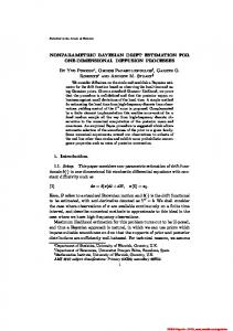
Fig. 1, the eigenvalues of the first four principal vectors are much bigger than that of the rest of the vectors, meaning that they account for most of the variation in the spike shape data set. Therefore, we decide to use the sub-space spanned by the first four dimensions, where we will estimate prior spike shape probability density function. As we can see from Fig. 2, the first four principal vectors look like spike shapes, but starting from the fifth shape, the vectors appear more like noise than real spike. This result agrees with the eigenvalues and endorses the selection of the first four principal vectors. Then we perform quantization. The entropy for each dimension of the reduced shape space is calculated, to determine the relative quantization levels of each dimension. The space is then quantized to obtain the p.d.f. p(s). Fig. 3 shows the marginal grids of the four dimensional quantization grid. Fig. 4 shows the 2-D marginal p.d.f.’s of the 4-D p.d.f. Fig. 5 shows the 1-D marginal p.d.f.’s of the 4-D p.d.f.
First Principal Shape
Second Principal Shape
0.4
0.4
0.3
0.2
0.3
0.1
Normalized amplitude
0.3
0.2
0.1
0
0.2
0.1
0
−0.1
0
−0.1
−0.2
−0.1
−0.2
0
20
40
60
80 100 120 Index of sample points
140
160
180
−0.3
200
0
20
40
(a) Principal shape 1.
60
80 100 120 Index of sample points
140
160
180
−0.2
200
0
20
40
(b) Principal shape 2.
Fourth Principal Shape
0.4
Third Principal Shape
0.5
0.4
Normalized amplitude
Normalized amplitude
0.5
140
160
180
200
160
180
200
Sixth Principal Shape
0.3
0.15
0.3
80 100 120 Index of sample points
(c) Principal shape 3.
Fifth Principal Shape
0.2
60
0.25
0.1
0.2
0.05
0.15
0.1
0
Normalized amplitude
Normalized amplitude
Normalized amplitude
0.2
0
−0.05
0.1
0.05
−0.1
0
−0.15
−0.05
−0.1
−0.2
−0.3
−0.2
0
20
40
60
80 100 120 Index of sample points
140
160
180
200
−0.25
−0.1
0
20
40
(d) Principal shape 4.
60
80 100 120 Index of sample points
140
160
180
−0.15
200
0
20
40
(e) Principal shape 5.
60
80 100 120 Index of sample points
140
(f) Principal shape 6.
Figure 2: First six principal shapes.
p(x )
p(x )
1
p(x )
2
0.09
p(x )
3
0.12
4
0.18
0.08
0.25
0.16 0.1
0.07
0.2
0.14
0.06
0.08
0.12 0.15
0.05
0.1 0.06
0.04
0.08 0.1
0.03
0.04
0.06
0.02
0.04
0.05
0.02 0.01 0 −10
0.02
−5
0
5 x1
10
15
0 −15
−10
−5
0 x2
5
10
0 −15
−10
−5
0 x3
5
10
15
0 −10
−5
0 x4
5
10
(a) Marginal pdf on principal axis(b) Marginal pdf on principal axis(c) Marginal pdf on principal axis(d) Marginal pdf on principal axis 1. 2. 3. 4.
Figure 5: 1-D marginal probability density function of the prior shape space.
−5
0
5
10
10 5 x
1
5 x1
10
5 x1
10
0
0
0
−5
−5
−5
x1 5
−10
−5
0 x3
5
10
5
−5
0
5
x2 −5
0
5
−5
−5
−10
−10
10
−10
−5
x
0 x
1
5
10
−5
0 x
5
3
500
4
10 5 x3
3
0
x
x3
0 −5
5
−5
−10
−5
0
5
10
0 x
−10 −5
−2000
0
−10
−5
x
0 x
5
−5
0 x
2
0
0
5
500
−1000
−1000
10
0 x
−2000
−5
−10
−5
5
−5 −10
−5
x2
0
5
0 x4
5
10
x3
Figure 3: Quantization of the spike shape space.
−1000 x
0
5
10
0
500
1000 1500
x 1500
1000
1000
1000
500
500
0
0 −500 −1000 x1
0
500 1000
−1000 −500
3
4
500 0
−500 −1000
0
0
500 x3
1000 1500
−500
1000
−1000 −500
x2 1000
0 x4
500 1000
0
500 1000
1000
500
0
500
x
0
0
5 x1
10
−5
0
5 x1
10
0
−500
−500
−1000
−1000
−1000
5
5
−2000
10 −5
0
x4
4
0 −500
−1000 −500 x
5
5
x1
−10 −5
0
5
x2
−10 −5
0 x2
5
−10
0 x3
10
−1000 x1
0
−1000
0
1000
−500
0
x2
500 x3
4
1000 1500
Figure 6: Quantization of the signal space.
Figure 4: Prior probability density function of the spike shape space. The 2-D marginal p.d.f.’s are actually shown. Representing the Evidence from Observed Spike Signals
3.
Results
3.1
Sorting on Simulated Spikes
We simulated a spike sequence of duration 7 seconds with 40kHz sampling rate. The spike sorting results of our algorithm are shown in Fig. 9. In this particular example, we had 15 miss-detected spikes and 5 false-alarm
−1500 −500
−1000
0
−500 x
x3
2
−500
4
−1000
x
0
500
500
1000
1000
0
500
1000
1500 −2000 −1500 −1000 −500 x1
0
500
−2000 −1500 −1000 −500 x1
0
500
−2000 −1500 −1000 −500 x1
−1000
−1000
0
−500
−500
500
1000
−1500 −1000
−500
0 x2
500
1000
500
x 0
0
500
500
1000
1500
0
4
−500
x4
When a stimulus produces spikes from a single neuron, the spikes tend to repeat themselves in similar shapes. The observed signal is a result of the spike shape with random noise. Therefore the repetitiveness of a similar signal is an indication of the existence of spike events. We perform space reduction and quantization similarly to p(s), except that the data are now in the signal space, rather than the shape space. Some signal vectors represent spike shapes and some do not. The signals are obtained by finding a maximum value and then taking two chunks of discrete signal samples before and after the maximum value. We denote these vectors by x. Therefore the conditional probability p(x|s) can be estimated. The following figures show the signal space density estimation for the signal “1channel40khz” channel one. Fig. 6 shows the marginal grids of the four dimensional quantization grid. Fig. 7 shows the 2-D marginal p.d.f.’s of the 4-D p.d.f. Fig. 8 shows the 1-D marginal p.d.f.’s of the 4-D p.d.f.
x3
2.3
0 x
−500
0
−1500 −500
1500
−2000
−5 x4
x4
0
10 −5
−5
−5 x3
4
x
3
x
x2
0 5
5
−1000
−10 −5
−5
0
−1000 −1500
2
500 1000
0 −500
0
500
−10
−5
1000
0 x4
500
0
1
1000
−10
−1000 −500
1000
1500
x3
x1
0
1000 1500
x3
5
500 x3
−500
x4
0
x3
−5
−5
0
500
0 −500
−1500
−5
−2000 −500
1000
x
0
x4
5
1000
1000
4
5
−1500
−2000 0 x2
−10
3
−500
−1000
−1500
−2000 −1000
5
5 x4
−1500
0
0
−500
−1000
1
10
2
1
x4
−1000 x
−5 −10
500
0
−500
−1000
x2
5
500
0
10 x1
10
5
x2
x −10
0 x4
0
2
0
x2
0 −5 −10
−5
5
x1
0 x2
x2
−5
x1
−10
5
−1500 −1000
1000 −500
0 x2
500
1000
−500
0
500
1000
1500
x3
Figure 7: 2-D marginal probability density function of the signal space.
p(x )
−3
2.5
p(x )
−3
1
x 10
3
3.5
p(x )
−3
3
x 10
3
3
2.5
2
p(x )
−3
2
x 10
4
x 10
2.5
2.5 2
2
1.5
2 1.5
1.5 1.5
1 1
1 1
0.5
0 −2500
0.5
−2000
−1500
−1000
−500 x
0
500
0 1000 −2000
0.5
−1500
−1000
−500
0 x
1
0.5
2
500
1000
0 1500 −1000
−500
0
500 x
1000
1500
0 2000 −1500
−1000
−500
3
0 x
500
1000
1500
4
(a) Marginal pdf on principal axis(b) Marginal pdf on principal axis(c) Marginal pdf on principal axis(d) Marginal pdf on principal axis 1. 2. 3. 4.
Figure 8: 1-D marginal probability density function of the signal space.
(a) Correctly detected spikes.
(b) A missed spike (the true one on the right in the bottom).
(c) A false-alarm spike (the false one on the right at the top).
Figure 9: Sorting results on simulated spikes. In each sub-figure, the red lines in the top signal represent the detected spike positions. The red lines in the bottom signal represent the actual position of the groundtruth spikes.
spikes for a total of 165 spike events. The average difference between the matched spikes is 0.068 millisecond with a standard deviation of 0.41 millisecond. 3.2
Sorting on Real Spikes
We performed spike sorting on a spike signal obtained from a monkey with 40 kHz. The sorting results are shown in Fig. 10, where the same spike signal is shown in different scales.
4.
Conclusion and Future Work
We have described a spike sorting approach based on a nonparametric density estimation technique under a Bayesian framework. A spike is detected based on the product of the prior probability of its shape and the probability of its repetitiveness in the observed signal. The two probabilities are obtained from the probability density functions of the prior shape space and the observed signal space, respectively, by a nonparametric quantization technique. We have demonstrated the performance of the software on a simulated spike signal and a real signal. In the case of the simulated spike signal, where the groundtruth is known, we are able to calculate the numbers of miss-detected and false-alarm spike events. Our results show that our approach is very promising. The fundamental reason is that we do not apply any restrictions on possible spike shapes, which is typically pre-assumed in other competing algorithms. Some future work includes using more groundtruth to build a better prior probability density function for the shape space. It also seems that including both relative magnitude and shape information might reduce the false-alarm spike events. We will also compare the performance of our algorithms with others.
References Hulata, E., Segev, R., & Ben-Jacob, E. (2001). A method for spike sorting and detection based on wavelet packets and Shannon’s mutual information. Journal of Neuroscience Methods, submitted. Lewicki, M. S. (1998). A review of methods for spike sorting: the detection and classification of neural action potentials. Network: Comput. Neural Syst.(9), R53-R78. Menne, K. M. L., Folkers, A., Malian, T., Maex, R., & Hofmann, U. G. (2002). Test of spike sorting algorithms on the basis of simulated network data. Neurocomputing, 44-46(C), 1119-1126. Oweiss, K. G., & Anderson, D. J. (2002). Spike sorting: a novel shift and amplitude invariant technique. Neurocomputing, 44-46(C), 1133-1139.
Sahani, M. (1999). Latent variable models for neural data analysis. Unpublished doctoral dissertation, California Institute of Technology, Pasadena, California.
(a) Detected spikes.
(b) Closer look.
Figure 10: Spike sorting algorithm on a real spike signal.
(c) Even closer look.