A pixel-based method to calculate the urban compactness and its preliminary application Jinqu Zhang Yunpeng Wang State Key Laboratory of Organic Geochemistry, Guangzhou Institute of Geochemistry, Chinese Academy of Sciences, Guangzhou 510640, China
[email protected] [email protected] Abstract: A pixel-based method was provided to calculate the urban compactness. Remote sensing technology was used to extract urban-used land information and the urban pixels in the classification image were directly used to calculate the urban compactness, which will be more proper. The method was basing on the assumption that the urban with a circle form is the most compact. 40 virtual circular cities with different radius were constructed to seek a formula to quantify the urban compactness. For each virtual city, 2 data can be acquired which are the circle area and the average distance (AD) of all the pixels to the circle center. Regression analysis shows that there is a good relationship between the urban area and the AD. The 40 data pairs of circle areas (y) and average distances (x) were used for regression analysis and it can be found that a curve function of y = 6.9351x2.0039 can simulate the points perfectly (r=1). Obviously, this curve is educed by countless virtual circular cities with different radius and the same compactness. Actually, for each real city in the classification image, a specific area and an average distance can be calculated directly. With the two specific data, there is one exclusive point and also there is one and only one curve with function of y = 6.9351xD passing the point. Studies showed that the value of D can be used to quantify the urban compactness. The method was applied to Dongguan city in the Pearl River delta, China and the compactness of Dongguan in the year of 1990 and 2003 were separately 1.76 and 1.87. The results accorded with the fact and showed the effect of the method. Keywords-urban compactness; pixels; classification image; pixel-based algorithm; Dongguan city
I.
INTRODUCTION
Urban compactness and directional extensibility reflect the urban morphology that is determined by both the natural environment, such as the terrain, and the human factors. In the forming of the urban spatial pattern, the city planners and the governors play an important role, while the urban spatial pattern affects people’s life on the other way round. As the population growth, sustainable development, which “meets the needs of the present without compromising the needs of future generations” has long been put forward. As far as the urban is concerned, a compact urban form should be paid more attention. Generally, the urban form is irregular and it is hard to give it an accurate description. In the previous studies, the urban form is mainly described qualitatively, which is hard to make an analysis between the urban form and some parameters such as urban environment conditions and urban population. And it
0-7803-9050-4/05/$20.00 ©2005 IEEE.
3833
is also difficult to give a comparison to the urban form by the time series. The urban form reflects the character of the urban development, so it should accord with the development of the urban economy and the social society, or it will block the social development. As the development of the geographic information system (GIS) and remote sensing (RS) technology and some other sciences such as computer and mathematics, urban form can be quantitatively expressed and many methods are proposed and put forward (Richhardson, 1961; Cole, 1964; Gibbs, 1961). The most widely used method is to choose a regular geometric shape such as a circle or a square as the frame of the reference so as to compute the specific value, which stands for the urban form. (Sonka et al.1993; Barnsley et al. 2003). Since the research to the length of the coastline in Britain made by Mandelbrot (1967), fractal analysis was proposed and was used to study the urban spatial distribution in Pearl River Delta and other areas (Batty & Longley, 1987, 1988; Qihao Weng, 2003). In the previous studies, GIS software is used as an important tool for analysis the urban form and the urban compactness is often calculated by the vector shape with the two parameters: perimeter and area. To some extent, it can be used to describe the urban form. But if the vector shape is converted from the remote sensing classification image, some uncertainties maybe occurred, because the urban area in the classification image is very fragmentized and not likely a whole one region. Maybe fractal analysis is probably suitable to describe this fragmentation of the urban area in the classification image, but not suitable to describe the urban compactness. White and Engelen (1993) used the area within a circle and the circle radius to compute the convergence of some land type. The objective of this paper is to provide a method to calculate the urban compactness directly from the remote sensing classification image. The method is based on one premise that the urban with a circle form is the most compact urban form. According to the urban area and the average distance of all the urban pixels to the center of the city, there will be one point corresponding to the city in the rectangular coordinates. A mathematic function curve passing the point is chosen to quantify the compactness of the city. Study shows that this method is effective and convenient. In the last, the method was applied to Dongguan, a city in the Pearl River Delta, which is one of the fastest growing regions in China, to detect the compactness changing from the year 1998 to the 2003.
3833
PRINCIPLES AND METHODOLOGY
A. Principle For a city in the classification image, the compactness is related with the distance of every urban pixel to the center of the city. Based on this, an average distance (AD) can be calculated for every city. If there are two cities with the same area, it is probably that the city with a smaller AD is more compact than the other with a larger AD. However, if the urban area is different, the more compact city may have a smaller AD, while the less compact city may have a larger AD. And the compactness could not be denoted by the AD of each city. So the urban area must be considered to quantify the compactness of a city. In order to find a method to calculate the urban compactness considering both AD and the urban area, 40 virtual cities with different AD and area were constructed. The 40 virtual cities are all have the circular urban form, that is to say, though they have the different AD and urban area, they all equally have the most compact urban forms. If we quantify the compactness of the 40 cities, the results will be the same. The AD and urban area of each virtual city was figured out and make up of 40 coordinates. Fig. X shows their positions in a rectangular coordinates. Regression analysis shows that the urban area and the AD have a highly correlated relationship, and all the city points were located on one curve which function can be expressed by y = 6.9351x2.0039, where y is the urban area and x stands for the AD (Fig.1). Based on this, the curve may be used to quantify the urban compactness. It not only considered the average distance, but also considered the urban area. Of course, the function y = 6.9351x2.0039 stands for the most compact urban form. In fact, for every city, there is an average distance and urban area, that is to say, one exclusive point corresponding to the city will be found in the rectangular coordinates. Because the point is exclusive for the city, if there is one and only curve passing the point, the curve could be then used to quantify the urban compactness. We know that the 40 virtual cities with the most compactness can be used a curve, which function is y = 6.9351x2.0039, to describe. If a similar function like y = 6.9351xD can be found, then a comparison could be made between different cities by the value of D. The key problem to make sure of the character of the function y = 6.9351xD. As function y = xD, different curves can be drawn according to the value of D (Fig. 2). When both the x and the y are bigger than one, the y will become bigger as the D grows bigger, that is to say in the gray area, the curve with a bigger value of D will be above the other curves with a smaller D value. Actually, when compute the urban area and the urban average distance in the classification image, the result of the area and the average distance must be bigger than one for the pixel is used as the unit and no city would be less than one pixel. If the x is considered as the average distance of all the urban pixels in the classification image to the center of the city and y as the urban area, the point (x, y) must locate in the gray area and there must be a exclusive curve which function likes y = 6.9351xD passing through the point. For the city, the value of D is unique and it will vary if the urban area or the average distances change. If the value of D is 2.0039, it is just the curve composed by the virtual cities having the most compact urban form. If we use the function y = 6.9351xD to simulate the urban
0-7803-9050-4/05/$20.00 ©2005 IEEE.
3834
point in the rectangular coordinates, D is the only variable to determine the function curve, and for every city point, there will be a specific D value corresponding to it. So the value of D can be used to quantify the compactness of the city to some extent. 6000000
Urban area (pixles)
II.
5000000
y = 6.9351x 2.0039 R2 = 1
4000000 3000000 2000000 1000000 0 0
200
400
600
800
Average distance (pixels) Fig.1 Relationship between AD and urban area Y 7 1.5
y = x
6 5 4
1
y = x
3 0.5
2
y = x
1
y = x
0
0 0
1
2
3
4
X
Fig.2 Curves of function y = xD B. Method As the development of remote sensing technology, the urban areas can be easily extracted by image classification. In the classification image, each class is endowed with a specific value of integer type and each pixel is fixed by its row and column coordinate. Based on the coordinates of each urban pixel, we can calculate the urban geometry center following the equations bellow (Eq.1; Eq.2)
CentreX
CentreY
=
=
n
1 n
∑
1 n
∑
(xi − 0)
i =1
n
i=1
( yi − 0)
(Eq.1)
(Eq.2)
3834
averD =
1 n ∑ ( xi − CentreX ) 2 + ( y i − CentreY ) 2 n i =1 (Eq.3)
Where averD is the average distance. Because the number of the urban pixels and the urban area has the absolute linear relationship and the average distance is also based on pixels, we use number of urban pixels stand for the urban area. When the averD and the urban area are figured out, the next task is to compute the value of D. In the function y = 6.9351xD, y is the urban area and x is the average distance, then the D become the only unknown variable. Changing the form of the function, we will get Eq.4. According to the last function, the value of D is easily figured out using the urban area and average distance (Eq.5). The D is just what we want. ln(y) = ln(6.9351) + D*ln(x) (Eq.4)
IV.
CONCLUSION
In the paper, the urban compactness was discussed and a pixel-based method was provided. The compactness of a city may be expressed in different ways and different methods reflect different aspects of the city. In our study, the compactness focused more on the urban spatial pattern and 160000 140000
y = 6.9351x
1.87
2003
120000 100000
1990
80000 60000
1 .76
y = 6.9351x
40000 20000 0 0
100
200
300
AD (pixels)
D=(ln(y) – ln(6.9351))/ln(x) (Eq.5) III.
the urban compactness will also be beneficial to the urban construction and the urban sustainable development.
Area (pixels)
Where Central X and Central Y stand for the coordinates of urban geometry center; n is the number of urban pixels; x and y standing for the row and column number. Here we use the (0,0) as the origin of the image. After the urban center is figured out, we can compute the average distance of all urban pixels to the urban center according to the following equation (Eq.3).
Fig.3 Points of Dongguan in 1990 and 2003
APPLICATION
The method was applied to Dongguan city in the Pearl River delta, China. During the past years, Dongguan has taken great changes, especially since the economic reform of China. From the year 1990 to 2003, the population of Dongguan increased more than 270 thousands and the GDP increased 105% per year for average (Guangdong year book). TM data of the year 1990, ETM+ data of 2003 were used for classification to extract the urban land information. In the study, supervised classification with the maximum likelihood algorithm was performed to classify the Landsat images using all bands except Band 6. According to the equations above (Eq.1; Eq.2), the urban center is (283, 321) in 1990 and (342, 289) in 2003. The average distance is 150.58 pixels for the year 1990 and 167.53 pixels for the year 2003. The urban area is 47898 pixels for the year 1990 and 101240 pixels for the year 2003. So the coordinates of the year 1990 and 2003 separately are (150.58, 47898) and (167.53, 101240) (Fig 3). According to the equations (Eq.4, Eq5) above, the value of D in 1990 is 1.76 and 1.87 for 2003. Two different curves standing for the compactness of Dongguang city in the year of 1990 and 2003 were figured out. It is clearly that the two curves passed the two points separately. The result shows that the compactness increased obviously from 1990 to 2003.
a. Urban-used land in 1990
The changing can also be founded from the classification image and Fig 4 was the urban-used land information extracted from the classification image of Dongguan in 1990 and 2003. By the method provided in the study, the compactness was computed and the result showed good consistency with the fact. According to the method provided in this paper, the urban compactness in 1990 and 2003 were 1.76 and 1.87, which can help us to give more analysis with other factors such as the population, rate of the economy. In fact, an in-depth study for
0-7803-9050-4/05/$20.00 ©2005 IEEE.
3835
b. Urban-used land in 2003 Fig.4 Urban-used land of Dongguan in 1990 and 2003
3835
the layout of the urban-used land. The compactness can be calculated directly from the classification image. Usually the classification image is converted into a vector file and then using the GIS software to compute the area and the perimeter, which are then used to analyze the urban spatial pattern, however the result of this method is affected by many uncertainties. In our study, the urban pixels in the classification image are directly used to calculate the urban compactness, which will be more proper. In fact, the city is 3-dimensional, so it would be more proper to consider the building height when compute the urban compactness. And also, the population density is also an important factor. Currently, the urban compactness is almost focusing on the urban shape or the spatial distribution of the urban-used land. The method is very necessary to give a further study. ACKNOWLEDGEMENTS This work was supported by Natural Science Foundation of Guangdong Province (Grant No. 04002143), Guangdong Science & Technology Project (Grant No. 2004A30401001) and National Key Basic Research Programming Project (973 Grant No. 2001CB209101). We want to greatly thank Prof. Anthony Yeh, Jiamo Fu, Qiguo Zhao for great support of this study.
0-7803-9050-4/05/$20.00 ©2005 IEEE.
3836
REFERENCES [1]
B. B. Mandelbrot. (1967). How long is the coast of Britain? Statistical self-similarity and fractional dimension. Science: 156, 636-638 [2] Barnsley, M., Steel, A., & Barr, S. (2003). Determining urban land use through an analysis of the spatial composition of buildings identified in LIDAR and multispectral image data. In V. Mesev (Ed.), Remotely sensed cities (pp. 83-108). London: Taylor & Francis. [3] Batty M. & longley P A. (1987). Fractal-based description of urban form. Environmental and Planning B: Planning and Design. 14:123-134 [4] Batty M. & longley P A. (1988). The morphology of urban land use. Environmental and Planning B: Planning and Design. 15:461-488 [5] Gibbs J. P. (1961). Urban research methods. New York. [6] Hiroyuki Yoshida, Manabu Omae. (2005). An approach for analysis of urban morphology: methods to derive morphological properties of city blocks by using an urban landscape model and their interpretations. Computer, Environment and Urban systems, 29, 223-247 [7] Qihao Weng, (2003). Fractal analysis of satellite-detected urban heat island effect. Photogrammetric Engineering & Remote Sensing, Vol. 69, No. 5, 555-566. [8] Richhardson H. W. (1973). The economics of urban size Lexington, Mass. [9] Sonka, M., Hlavac, V., & Boyle, R. (1993). Image processing, analysis and machine vision. London: Chapman & Hall. [10] White R. & Engelen G. (1993). Cellular automata and fractal urban form: a cellular modelling approach to the evolution of urban land-use patterns. Environmental and Planning A, (25), 1175-1199.
3836