A Predictive Sensor Network Using Ant System Rajani Muraleedharan and Lisa Ann Osadciw Department of Electrical Engineering and Computer Science Syracuse University Syracuse, NY 13244-1240 (315) 443-1319 (office)/(315) 443-2583 (fax) rmuralee,
[email protected] ABSTRACT The need for a robust predictive sensor communication network inspired this research. There are many critical issues in a communication network with different data rate requirements, limited power and bandwidth. Energy consumption is one of the key issues in a sensor network as energy dissipation occurs during routing, communication and monitoring of the environment. This paper covers the routing of a sensor communication network by applying an evolutionary algorithm - the ant system. The issues considered include optimal energy, data fusion from different sensor types and predicting changes in environment with respect to time. Keywords: Communication, Swarm Intelligence[1], Ant System, Data Mining[2, 3], Sensor Network
1. INTRODUCTION A building consists of a sensor network with a multitude of wireless communication links and the sensors are interconnected by means of RF communication links. The functionality of nodes in this application include sensing, collecting and distributing dynamic information within the network. Energy usage is a key issue as the sensors are typically tiny and wireless with limited memory and functionality given the fact that the batteries(y) have a limited power supply hence difficulties arise during computation[4]. The communication links in such an unpredictable environment (node failures) are kept functional by applying a robust routing algorithm. The Ant system is a learning algorithm with characteristics such as robustness and versatility solves any NP hard communication problem. In this paper a novel approach is proposed. The agents use the sensor node’s information to determine patterns to predict or anticipate changes in the environment with respect to time. The swarm agents are distributed along the network, where the agent communicates with its neighbors (agents). The current information on energy usage, prediction and decisions concerning environmental situation assessment are made possible by these swarm agents. Another optimization issue is the communication delay. During individual node failure, the swarm routing, unlike some other types of routing, automatically reroutes messages around node failures. The only data lost is data that was last prepared by the node or collected and processed by the failed node. The new route is determined by applying the link status to the ant routing algorithm and other factors depending on the performance parameters including energy and distance. An evolutionary algorithm may not always provide the best global solution but does find the best local decision. Optimality[5], finding the solution that finds the best performance, and reachability[5], the global optimal is found instead of the local optimal, are the two important factors in choosing an appropriate algorithm. The focus of this paper, is to determine patterns using sensor node’s information to predict or anticipate changes in the environment with respect to time. In the second section, the justification for using ant system and its impact on the sensor network is discussed. Section 3 discusses data mining and its importance in making predictable decisions to improve the performance of the network. Simulation results provide an insight of real-time situation assessment are provided in the fourth section. The paper concludes with the fifth section discussing the conclusion and future work.
2. SWARM INTELLIGENCE AND ANT SYSTEM Swarm Intelligence, is an algorithm that models the collective behavior of social insects, namely the ants, bees, birds, slime mould, etc. Ant system is one such evolution from the swarm intelligence forming an evolutionary algorithm with unique characteristics such as robustness, distributed problem solving, versatility and de-centralized approach. The ant system solves any complex optimization problem involving many complex and heterogeneous nodes. It also adapts to the network with environmental changes. The agents in the system communicate interactively either directly or indirectly in a distributed problem-solving manner. In this paper, the ant system is applied to a building sensor network with wireless sensor nodes. The agents move towards the optimal solution and communicate directly by sharing knowledge with their neighbors. The initial set of agents traverse through the nodes in a random manner, and once they reach their destinations, they deposit pheromone trails as a means of communicating indirectly with the other ants. The pheromone accumulation is proportional to the number of agents traveling between two nodes during one complete iteration. The amount of pheromone left by the previous ant agents increases the probability that the same route is taking during the current iteration. Other performance factors discussed also affect the probability of selecting a specific path or solution. Pheromone evaporation over time plays an important role in preventing suboptimal solutions from dominating in the beginning. There are three different kinds of ant agents, which performs functions such as allocating, sensing and de-allocating the sensed values. Thus, no values are fed into the system other than the initial values. In the system, the agents minimize energy and keep track of network requirements. The allocator agents monitor the allocation process on active links and allocate resources required by the network. The sensing agent’s function is to traverse the network and communicate with its neighbors to reach the destination using an optimal route. The deallocator agents are responsible for deallocating trails identified by the sensing agents with the sensed values. As the ant moves from node to node, energy is lost through communication. The ant stops traversing a node once its energy is depleted. New paths are set up to avoid the node so that communication continues without the degraded sensor. These agents ensure that the optimal route to the destination using limited resources and also learning the network environment. Initially, the computational cost and time is high but this drops drastically once the agents learn the network and environment A Tabu-list serves as memory tool listing the set of nodes that a single ant agent has visited. The ant’s goal is to visit nodes in the network depending on the number of hops assigned by the user. Thus traversing all the nodes and depleting all the energy at every node is avoided. The pheromones on all the paths are updated at the end of a tour. The pheromone deposition, tabu-list, and energy monitoring help this novel ant system (AS) to obtain a optimal solution and adapt it as nodes degrade. 2.1 Ant System in a Building Sensor Network Figure 1 shows a sensor network incorporated for a four-storey building layout. The circles denote sensors, which are placed in the rooms. The number of rooms in the building is independent of the number of sensors. The environment inside the building is monitored for safety as well as security purposes. For instance, sudden raise in temperature in any room or hallway indicates an emergency situation, so assessing the situation and monitoring all movement in a building proves valuable. The amount of false alarms can also be reduced by fusion of data at sensor nodes. The nodes help in transferring effective data for making decisions. The energy of each sensor and their communication strength varies depending on the presence of any major obstacles in the routing path
Fig. 1.Four storey building layout with wireless sensors
A suboptimal tour is represented in Figure 2 with circles denoting the nodes and the lines denoting the paths taken by the ant agents between the sensor nodes within a floor. The dotted arrowed lines represent communication between floors in the building. Floors 1, 2, 3 and 4 are spread with 6, 7, 6 and 6 sensors, respectively. In each floor, the source and destination nodes are varied but the number of hops 5 remains constant. Communication among nodes between Floor 1
Floor 2
Floor 4
Floor 3
Fig. 2.Suboptimal routes taken by the ant agent upon traversing sensor’s in the building
floors is proportional to the strength between the links. Hence, there are no cluster heads in the sensor network. The node locations are represented in dimensional cartesian coordinates for this simulation. The nodes are initially assigned with random energy value. Three key elements in this AS include the pheromone deposition, energy tracking, and tabu list maintenance. There is a loss of energy that is the reciprocal of the distance between the nodes travelled by the agent. The tour begins at the specified source node in the Figure 2 and ends when a route is complete in regard to the number of hops and finally reaching the destination node. In a given tour, a node is never re-visited. A particular node could be ignored if the fused information is found in the neighboring node or if the number of hops is achieved. The Tabu list contains a record of the path taken by each agent. The pheromones are updated and the list is cleared after completion of each tour. The change in pheromones is a function of the amount of pheromone deposited on the path, the total distance travelled by the agent and the weight applied to the mined information of the link status. The mathematical approach of the ant system in a building sensor network is given in detail in the following section. 2.2 Mathematical Approach Of the Ant System The performance of the AS is determined by the node spacing and 4 parameters: Q is an arbitrary parameter, ρ , controls trail memory, α is the power applied to the pheromones in probability function, and β is used as the power of the distance in probability function. These AS parameters control the performance of the ant system on a specified set of nodes. The Euclidean distance D ij =
2
( X i – X j ) + ( Y i – Yj )
2
where i is the source node, j is the destination node, and
(Xi,Yj) are the cartesian coordinates of the node. The ant agents accumulate pheromones and dissipate energy as they traverse through the nodes based on the path probabilities. The pheromone is initialized and is assigned value of 10. The pheromone is updated following each complete tour by, (AS - see [7, 8, 11, 12]) Q ψ ij ( t ) = ρ ( ψ ij ( t – 1 ) ) + --------------Dt ⋅ Et
(1)
where Dt is the total distance travelled by ant agents during the current tour, i is the index for the source node with coordinates (Xi,Yi), and j is the index for the destination node with coordinates (Xj,Yj). The transition probability between nodes for a wireless network is computed from with its neighbors (agents) by means of pheromone deposition and tabu list . Pij
α 1 2β α ( Ψ ij ) ⋅ ------- ⋅ ( E ij ) D ij = -----------------------------------------------------------------------1 2β α ( Ψ ) α ⋅ ------⋅ ( E ) ik ∑ ik Dik
(2)
k
The energy is dissipated from the sensor node after each ant passes through that node. Assumption is made that the wireless nodes consumes more energy than of a wired network. Thus the distance is squared and the energy for a wireless sensor node is given by, K ∆ E ij = -------------2D ( i j)
(3) The link budget k, is calculated with respect to the bluetooth protocol i.e., where Ptx is the transmitted power, Gtx and Grx are the antenna transmit and receiver gain, Lfs is the propagation loss and Prx is the receiver sensitivity. Ptx = Prx – G tx + L fs + Fadem arg in
The node’s remaining energy is computed by
(4)
E ( t) = E ( t – 1) – ∆ E i i ∑ ij
j (5) The agents avoid visiting nodes with depleted energy by determining alternative routes in the sensor network. Thus the network remains partially functional even if some individual sensors fail. The tabu list supports energy usage prediction and decisions concerning situation assessment. Transition probabilities assist in optimizing route selections. The above features of the ant system coupled with data mining enhances the predictive nature of sensor network as discussed in the future sections.
3. DATA MINING & SENSOR NETWORK Data mining is the result of natural evolution of information technology. A non-trivial extraction or mining knowledge of previously known and potentially useful information from a collection of data set. Data mining is applied in many fields for valuable information assessment[13]. In this paper, a sensor network where decision is one of the key factor for any action to take place, it plays a vital role in situation assessment. Data mining works with different kinds of databases, for a network analysis spatial and heterogeneous datasets are used. 3.1 Data Mining With Ant System The computation complexity of data mining for large database is O(np3), where n data points and p is the associated measurement. Thus the need for a global optimization becomes necessary. There are many algorithms combined Information Retrieval
Statistics
Database Data Mining
Machine Learning Algorithm
Fig. 3.Data mining as a confluence of multiple disciplines
with data mining to obtain optimal solutions, one such evolutionary algorithm is ant stem (AS). The probabilistic way of obtaining a solution has proven better for large and complex databases. The rules used for mining the data from the data set is performed by the AS. Using the updated information on the energy depletion and physical distance between nodes the link status can be predicted. The agents deposit the pheromones on the path which is proportional to the predicted link status. The pheromone value corresponds to the greater probability of choosing a stable route. The obtained solution is added to the empty list, which in other words is the tabulist with the link status. The mined data stored in the tabu-list serve as a base for future data analysis.
4. PREDICTIVE SENSOR NETWORK USING ANT SYSTEM AND DATA MINING The sensor network with 9 nodes in each floor is considered, with the suboptimal route of a single floor as given in Figure 4. Data fusion[14] occurs at each node so that the environment information is always current. In addition, the agents use sensor node’s information to determine patterns that are used to predict or anticipate changes in the environment with respect to time. S1 S2 S0
S5
S4
S3 S7
S8
S6
Fig. 4.Predictive Sensor Network Using Ant System and Data mining
The number of hops assigned for this network is 5. The route taken by the agent1 denoted by bold lines is among nodes S0, S3, S2, S5, S7 to S8. The fusion of data is denoted as dotted arrowed lines between nodes S1 and S2 ignoring S1, the data at S4 is fused with S3 eliminating S4 out of the route. The fusion of data between S6 and S7 eliminates S6 out of the communication path. The fused data provides precise information about the particular environment under the sensor’s line of sight. The fused data also helps in making simple predictions for data mining rather than increasing complexity in data set. 4.1 Detailed Approach - Predictive Sensor Network The Sensor network is made predictive, robust and versatile by applying ant system and data mining, which provides effective situation assessment. The probabilistic approach of the ant system depends on the energy depletion and the percentage of false decision. The two factors need to be minimal. Figure 5 provides a pictorial description of the algorithm used in making a predictive sensor network. The manual operation involved in this network is the definition of the building layout, the sensor equipped in each floors and the initial parameters used in the ant system. The number of agents is proportional to the number of sensors used in the building sensor network. The ant agents are randomly placed on the sensors, not all sensor nodes are assigned an agent. The agents are iterated till the user specified criteria is reached. As discussed in the second section, the three key elements of the ant system play an important role in making the network robust and de-centralized. The information on the resource availability at any node helps in predicting the link for the agent’s next visit.
Initialize Building Layout, # Sensors,
Set Ant agent parameters, Thresholds at each node
Y
I < = # iterations
Until # hops for all agents
Minimal Energy, # Active links, Minimal Distance
N
N
A
Y Compute Transition Probability
Move ant to the next node
A
Update Pheromone
Update Tabu List with Energy, Route taken and Distance Predict Link Status & Update Tabu-List
Fig. 5.Flowchart - Predictive Sensor Network
The transition probability is the key factor for making decisions. Weights on each of the factors affects the movement of the ant agent in the network. Link factor is incorporated into the ant system. The transition probability is given as
Pij
· β α α α 1 2β ( ( ψij ) ⋅ ( Hop ij ) ⋅ ( E ij ) ⋅ ( Link ij ) ) ⋅ ------- D ij = -----------------------------------------------------------------------------------------------------------------------------β α 1 2β α α ------( ( ) ⋅ ( Hop ) ⋅ ( E ) ⋅ ( Link ) ) ⋅ ψ ik ik ik ∑ ik D ik
(6)
k
where Linkij is the normalized link status as in (7). Hopij (8) is the normalized value of the total and actual hops taken in a route. The two factors help in making decisions while traversing the data set formed by the agents.
· ( TotalLinks – UnhealthyLinks ) Link = ---------------------------------------------------------------------------------TotalLinks · ( Totalhop – ActualHop ) Hop = --------------------------------------------------------------Totalhop
(7) (8)
The link status in a tour taken by an agent is incorporated in the pheromone (9). Thus the trails formed by the ant agent is now dependent on the link factor. The pheromone deposition is defined as Q ψij ( t ) = ρ ( ψij ( t – 1 ) ) + -------------------------------------------------D t ⋅ Et ⋅ Link t ⋅ Hop t
(9)
The tabu list now consists of updated values of the energy available in the nodes for the particular sub-optimal route with high reachability. 4.2 Result A sensor network with 16 nodes is considered in this simulation run with agents randomly placed on the nodes. After converging, the ant agents adapt to the network using the knowledge acquired from their neighbors. The table below illustrates six scenarios where the predictive nature of the algorithm is used for assessing the performance of the network. The parameters of ant system are assumed to be α = 4, β = 7, ρ= .7, Q = 9 and initial pheromone value, ψ as 10. The number of agents employed in the network is 16, and the source and destination nodes were assumed constant. The stability of the algorithm is analyzed by iterating all scenarios for 100 runs. The total hops for all the simulations given below is assumed to be 16 which is the number of nodes in the network. The actual hops is user defined which varies depending on the problem assigned. The normalized value of hops is given as HopsNorm. The total number of links in the network is equal to the total hops in the network. The normalized link value is given as LinkNorm. The predicted energy and distance helps in making a decision whether the nodes in the current route is still capable of communicating with its peers in the next iteration. Table 1 shows the performance of the sensor network where two link failure is estimated. The actual hop is set as 1 with 2 unhealthy and the predicted energy obtained is 82.664. The very high energy prediction leads to a lesser probability of the route to be chosen. In the worst case, where the actual hop is 10, total links is 14, the predicted energy is 43.909. Hence the probability of choosing this route is very high. Thus the network is kept functional even at the worst case. Table 1. Performance of Sensor Network - Link Failure - 2 Nodes
# Total Hops
# Actual Hops
HopsNorm
# Total Links
# Unhealthy Links
LinkNorm
Predicted Distance
Predicted Energy
16
1
0.9375
16
2
0.875
20.1465
82.664
16
2
0.875
16
2
0.875
18.8406
76.658
16
4
0.75
16
2
0.875
22.3657
74.254
16
6
0.625
16
2
0.875
21.6523
51.526
16
8
0.5
16
2
0.875
23.7393
47.771
16
10
0.375
16
2
0.875
23.9534
43.909
The unhealthy links are rounded to the highest value with respect to the actual number of hops involved to enforce 50% link failure as shown in Table 2. When half of the unhealthy links is equal to the actual number of hops 4 and 6, the energy for the next route is predicted falls between 43.528 and 47.147 respectively. As the number of unhealthy links are increased with respect to the actual number of hops, the energy predicted is also reduced. Thus for a minimal unhealthy link the predictive energy is 62.785. The number of hops plays an important role in leading to a reduced predictive distance and energy. Under a high predictive distance and reduced predictive energy, even the 50% link failure could be overcome. Table 2. Performance of Sensor Network - Link Failure - 50%
LinkNorm
Predictive Distance
Predictive Energy
1
0.9375
21.3592
62.785
16
1
0.9375
23.6468
55.212
0.75
16
2
0.875
20.5850
43.528
6
0.625
16
3
0.8125
18.4669
47.147
16
8
0.5
16
4
0.75
24.2436
48.059
16
10
0.375
16
5
0.6875
20.9937
55.934
# Total Hops
# Actual Hops
HopsNorm
# Total Links
# Unhealthy Links
16
1
0.9375
16
16
2
0.875
16
4
16
Table 3 gives the performance of the sensor network where the distance between all the nodes is evenly distributed. The equi-distant node placement results in uniform energy dissipation among the nodes. When the link failure was estimated as 50%, as the nodes where equi-distant, the distance predicted remains a constant at 15. There is only a slight energy variation with respect to the number of actual hops. Hence for a equi-distant network even when most of the link fails the performance of the network remains better. Table 3. Performance of Sensor Network - Distance Evenly Distributed- Link failure - 50%
LinkNorm
Predictive Distance
Predictive Energy
1
0.9375
15
45.301
16
1
0.9375
15
44.694
0.75
16
2
0.875
15
44.564
6
0.625
16
3
0.8125
15
45.722
16
8
0.5
16
4
0.75
15
44.630
16
10
0.375
16
5
0.6875
15
45.529
# Total Hops
# Actual Hops
HopsNorm
# Total Links
# Unhealthy Links
16
1
0.9375
16
16
2
0.875
16
4
16
Table 4 gives the performance of the sensor network where the distance between all the nodes are unevenly distributed. Hence, the performance of the network is counted towards all the three factors distance, energy and link status between the sensors. As the nodes are placed at random, the energy dissipation between the nodes is also random. Hence, the number of link failure is assumed to be 50% with fusion between nodes that have healthy communication links but not included in the route. When the actual hop is 4 and the number of healthy link is 13, the predictive distance and energy is 22.1076 and 62.439 respectively. The unevenly distributed network fails to function when the number of unhealthy link is increased to 8. The predictive distance though being minimal 21.9813 results in very high predicted energy of 85.696, that the route becomes inefficient for traversing.
Table 4. Performance of Sensor Network - Distance Unevenly Distributed - Link failure 75% - With Fusion
# Total Hops
# Actual Hops
HopsNorm
# Total Links
# Unhealthy Links
LinkNorm
Predictive Distance
Predictive Energy
16
1
0.9375
16
1
0.9375
21.1744
46.741
16
2
0.875
16
2
0.875
24.0675
54.883
16
4
0.75
16
3
0.8125
22.1076
62.439
16
6
0.625
16
5
0.6875
21.1052
47.711
16
8
0.5
16
6
0.625
21.1318
53.028
16
10
0.375
16
8
0.5
21.9813
85.696
Table 5 gives the performance of the sensor network where the energy at each node is evenly distributed. Hence, the performance of the network is counted towards the distance, energy dissipation and link status between the sensors. As all the nodes have same energy level, but random energy dissipation, the link failure could be problem dependent. The problem is made simple by considering only 50% link failure. When the number of unhealthy links is half the number of hops i.e., 1:1 ratio the predictive energy is very high 62.164, 75.145 and 60.061 respectively. For a uniform energy distribution, the communication strength due to energy dissipation at each node varies and may lead to less or high energy prediction with a minimal distance of 19.7592. Table 5. Performance of Sensor Network - Energy Evenly Distributed - Link Failure 50%
# Total Hops
# Actual Hops
HopsNorm
# Total Links
# Unhealthy Links
LinkNorm
Predictive Distance
Predictive Energy
16
1
0.9375
16
1
0.9375
20.9240
62.164
16
2
0.875
16
1
0.9375
21.6365
46.669
16
4
0.75
16
2
0.875
23.1213
56.104
16
6
0.625
16
3
0.8125
22.5765
43.550
16
8
0.5
16
4
0.75
19.7592
75.145
16
10
0.375
16
5
0.6875
21.7883
60.061
Table 6 gives the performance of the sensor network where the energy at each node is unevenly distributed. Hence, the performance of the network is counted towards the distance, energy and link status between the sensors. As all the nodes have random energy level and also the energy dissipation is unpredictable, the link failure could be problem dependent. The problem is made simple by considering only 75% link failure with respect to the actual number of hops.The predictive energy is very high at 95.05 as the link failure is equal to the number of links available. In a network with 75% node failure, data transfer becomes crucial. In such cases, even if the energy predicted is 86.43, 87.22 with only one node healthy link and 74.09, 75.28 with two healthy nodes, the routing is still made possible.
Table 6. Performance of Sensor Network - Energy Unevenly Distributed - Link Failure 75% - With Fusion
# Total Hops
# Actual Hops
HopsNorm
# Total Links
# Unhealthy Links
LinkNorm
Predictive Distance
Predictive Energy
16
1
0.9375
16
1
0.9375
22.1074
95.00
16
2
0.875
16
2
0.875
20.5627
86.05
16
4
0.75
16
3
0.8125
21.1788
85.43
16
6
0.625
16
5
0.6875
24.5108
87.22
16
8
0.5
16
6
0.625
23.2495
74.09
16
10
0.375
16
8
0.5
21.3214
75.28
5. CONCLUSION AND FUTURE WORK This paper proposed a predictive sensor network where energy, distance, number of hops and the link status were considered as the key factors combined in an evolutionary algorithm with data mining. The network under a 75% node failure is shown to be functional indicating the robustness of the Ant system. The six scenarios presented in the result section re-emphasize the fact that a sensor network remains functional and assess the situation under all critical conditions. The sensor network considered in this paper is made simple with 16 nodes and ant agents. The algorithm works on heterogeneous sensor network by only modifying the initial set up of the algorithm. In future work, the data collected by the sensor nodes is made as a dataset from which both an assessment and suggesting a plan based on the situation could be predicted. A sensor network with predictive nature could be applied to many applications where decision plays an important role such as medical controller, military applications, traffic monitoring and others.
REFERENCES 1. Kennedy J, Shi Y. and Eberhart R.C., “ Swarm Intelligence ” , Morgan Kaufmann Publishers, San Francisco, 2001. 2. Jiawei Han, Micheline Kamber, “ Data Mining Concepts and Techniques “ , Morgan Kaufmann Publishers, 2000. 3. M. Weiss and C. A. Kulikowski, “ Computer Systems that Learn - Classification and Prediction Methods from Statistics, Neural Nets, Machine Learning, and Expert Systems “, San Francisco, Morgan Kaufmann Publishers 4. Rajani Muraleedharan and Lisa Ann Osadciw, “ Balancing The Performance of a Sensor Network Using an Ant System “, 37th Annual Conference on Information Sciences and Systems, John Hopkins Unversity, 2003. 5. Rajani Muraleedharan and Lisa Osadciw, “Sensor Communication Networks Using Swarming Intelligence”, IEEE Upstate New York Networking Workshop, Syracuse University, Syracuse, NY, October 10, 2003. 6. Mansi P. Narkhede, Rosano S. Silveira and Lisa Ann Osadciw, “ Adaptive Modulation and Error Control for Energy Efficiency for Wireless Smart Card “, 37th Annual Conference on Information Sciences and Systems, John Hopkins Unversity, 2003.
7. Luca Maria Gambardella and Marco Dorigo, “ Solving Symmetric and Assymetric TSPs by Ant Colonies“, IEEE Conference on Evolutinary Computation(ICEC’96), May20-22,1996, Nagoya, Japan. 8. Marco Doringo, “The Ant System: Optimization by a Colony of Cooperating Agents“, IEEE Transactions on Systems, Man and Cybernetics-Part B, Vol-26, No. 1, Sept1996, pp 1-13. 9. Dorigo and L.M. Gambardella, “ Ant colony system: a co operative learning approach to the travelling salesman problem” , IEEE Transations on Evolutionary Computation, Vol 1, no.1, 1997, pp.53-66, JOURNAL. 10. Yun-Chia Liang and Alice E. Smith, “ An Ant system approach to redundancy allocation," Proceedings of the 1999 Congress on Evolutionary Computation, Washington D.C., IEEE, 1999, 1478-1484.8] 11. H. Van Dyke Parunak,” Go To The Ant: Engineering Principles from Naturla Multi-Agent System”, Forthcoming in Annals of Operations Research, special issue on Artificial Intelligence and Management Science, 1997, pp. 69-101. 12. H. Van Dyke Parunak, Sven Brueckner, “ Ant like Missionaries and Cannibals : Synthetic Pheromones for Distributed Motion Control ”, Proc of the 4th International Conference on Autonomous Agents(Agents 2000), pp. 467474. 13. Rafael S. Parpinelli1, Heitor S. Lopes1, and Alex A. Freitas, “ Data Mining with an Ant Colony Optimization Algorithm “, Proc of the 2002 IEEE International Conference on Evolutionary Computation, special issue on Ant colony optimization. 14. Lisa Osadciw, Pramod K Varshney, Kalyan Veeramachaneni, "Optimum Fusion Rules for Multimodal Biometrics in the book titled " Multisensor Surveillance Systems: The Fusion Perspective", Kluwer Academic Publishers. 15. Kennedy J and Eberhart R. C., “ Particle Swarm Optimization “, Proc of the 1995 IEEE International Conference on Neural Networks, vol 4, IEEE Press, pp. IV: 1942-1948. 16. Shi Y. and Eberhart R.C., “ Empirical Study of Particle Swarm Optimization “, Proc of the 1999 IEEE International Conference on Evolutionary Computation, Vol 3, 1999 IEEE Press, pp 1945-1950. 17. Barry Brian Werger and Maja J Mataric, “ From Insect to Internet: Situated Control for Networked Robot Teams “, Annals of Mathematics and Artificial Intelligence, 31:1-4, 2001, pp. 173-198.