4â17, 2002. [5] A. Abran, R. Al Qutaish, J. Desharnais, and N. Habra, ISO-based Models to Measure Software Product Quality. Institute of Chartered Financial.
A Probabilistic Software Quality Model Tibor Bakota, Péter Heged˝us, Péter Körtvélyesi, Rudolf Ferenc, and Tibor Gyimóthy University of Szeged Department of Software Engineering Árpád tér 2. H-6720 Szeged, Hungary {bakotat,hpeter,kortve,ferenc,gyimothy}@inf.u-szeged.hu
Abstract—In order to take the right decisions in estimating the costs and risks of a software change, it is crucial for the developers and managers to be aware of the quality attributes of their software. Maintainability is an important characteristic defined in the ISO/IEC 9126 standard, owing to its direct impact on development costs. Although the standard provides definitions for the quality characteristics, it does not define how they should be computed. Not being tangible notions, these characteristics are hardly expected to be representable by a single number. Existing quality models do not deal with ambiguity coming from subjective interpretations of characteristics, which depend on experience, knowledge, and even intuition of experts. This research aims at providing a probabilistic approach for computing high-level quality characteristics, which integrate expert knowledge, and deal with ambiguity at the same time. The presented method copes with “goodness” functions, which are continuous generalizations of threshold based approaches, i.e. instead of giving a number for the measure of goodness, it provides a continuous function. Two different systems were evaluated using this approach, and the results were compared to the opinions of experts involved in the development. The results show that the quality model values change in accordance with the maintenance activities, and they are in a good correlation with the experts’ expectations. Index Terms—ISO/IEC 9126, Software Quality, Quality Model, Software Maintainability.
I. I NTRODUCTION Both for software developers and managers it is crucial to have clues about different aspects of the quality of their systems. The information can mainly be used for making decisions, backing up intuition, estimating future costs and assessing risks. The ISO/IEC 9126 standard [1] defines six high-level product quality characteristics which are widely accepted both by industrial experts and academic researchers. These characteristics are: functionality, reliability, usability, efficiency, maintainability and portability. The characteristics are affected by low-level quality attributes which can be internal (measured by looking inside the product, e.g. by analyzing the source code) or external (measured by execution of the product, e.g. by performing testing). Maintainability is probably the most attractive, observed and evaluated quality characteristic of all. The importance of maintainability lies in its very obvious and direct connection with the costs of altering the behavior of the software. Although, the quality of source code unquestionably affects maintainability, the standard does not provide a consensual set of source code measures as internal quality attributes. The standard also does not specify the way how the aggregation of quality
attributes should be performed. These are not deficiencies of the standard, but it offers a kind of freedom to adapt the model to specific needs. Many researches took the advantage of this freedom and a number of practical quality models have been proposed so far [2]–[6]. Most of these researches share some basic principles: 1) In the case of each considered source code metric, its distribution over the source code elements is taken and a number (e.g. average) or a category (based on threshold values) is used for representation. 2) The number or category is aggregated “upwards” in the model by using simple weighting or linear combination. 3) Higher quality characteristics are also represented by one number or a category. Our intention in this paper is also to exploit the freedom of the standard and to propose a novel approach which is fundamentally different from the existing ones. We expect a quality model to satisfy the following requirements: 1) Interpretable – applying the model should provide information for high level quality characteristics which is meaningful, i.e. conclusions can be drawn with the help of it. 2) Explicable – there should be a way to efficiently evaluate the root causes, i.e. a simple way to decompose information obtained for high level characteristics to subcharacteristics or even to attributes. 3) Consistent – the information obtained for higher level characteristics should not contradict to lower level information. 4) Robust – the model should provide valuable information even for large systems in reasonable time. 5) Extendible – there should be an easy way to extend the model with new quality attributes and characteristics. 6) Comparable – information obtained for quality characteristics of two different systems should be comparable and should correlate with the intuitive meaning of the characteristics. By applying probabilistic methods, the approach – presented in this paper – conforms to all our requirements and eliminates many of the drawbacks of the current approaches that follow the basic principles. Our main contributions described in this paper are the following:
We defined a probabilistic model for evaluating high-level quality characteristics for software systems by aggregating low-level attributes to higher levels. • We applied this model to two software systems and showed that the model correlates with experts’ quality feelings quite well. The remaining sections of the paper are organized as follows. Section II outlines related work. Then, Section III discusses the mathematical background of our approach. Afterwards, Section IV shows the application of the approach by creating a quality model for Java systems and presents the results and the evaluation of the model. Section V collects the threats to validity of our work. Finally, we conclude the paper and present future work in Section VI. •
II. R ELATED W ORK The appearance of the widely accepted ISO/IEC 9126 and connecting standards [1] has pushed forward the research in the field of quality models. Numerous papers, ranging from highly theoretical to more practical ones, are dealing with this unavoidable research area. Some of the research focus on developing a methodology for adapting the ISO/IEC 9126 model in practice [7]–[9]. They provide guidelines or a framework for constructing effective quality models. We focus more on presenting an algorithmic approach and a particular application of it for evaluating software quality based on source code metrics. Other papers deal with software quality from the end user’s point of view. For example Ozkaya et al. [10] emphasize the importance of using quality models like ISO/IEC 9126 in practice right from the beginning of the design phase. Although the approach presented in their paper is general enough for evaluating design or end-user quality, in this paper we focus on source code (i.e., product) quality evaluation. Jung et al. [11] conducted a survey to reveal the correlation among subcharacteristics of the ISO/IEC 9126 standard. They showed that the highly correlated subcharacteristics according to the users’ opinion are different from the ones defined by the standard. We also prepared a survey to validate our approach, the difference is that we used this information to show the usefulness of the model and not to evaluate the correlations among the characteristics of the standard. Research of Bansiya and Davis [4], and Muthanna et al. [3] focus on the software design phase. They adapted the ISO/IEC 9126 model for supporting quality assessment of system design. Contrary to their approach, our model is based on low level source code metrics instead of design level metrics and aims at assessing product quality of an already existing system. Moreover, they use simple linear combination for evaluating high level characteristics while we apply a probabilistic approach and use a large benchmark of systems as reference instead of calculating absolute values directly. Kuipers and Visser introduced a maintainability model [12] as a replacement of the Maintainability Index by Oman and Hagemeister [13]. Based on this work Heitlager et al. [2], members of the Software Improvement Group (SIG) proposed
an extension of the ISO/IEC 9126 model that uses source code metrics at low level. Similarly to ours, their paper also focuses on the Maintainability characteristic of the standard. Metric values are split into five categories, from poor (--) to excellent (++). The evaluation in their model means summing the values for each attribute (having the values between -2 and +2) and then aggregating the values for subcharacteristics. Therefore, their model is capable of assessing the product quality (maintainability) of a software on a scale of five. Correia and Visser [14] presented a benchmark that collects measurements of a wide selection of systems. This benchmark enables systematic comparison of technical quality of (groups of) software products. Alves et al. [15] presented a technique for deriving metric thresholds from benchmark data. This method is used to derive more reasonable thresholds for the SIG model as well. Correia and Visser [16] introduced a certification method that is based on the SIG quality model. The method allows us to certify technical quality of software systems. Each system can get a rating from one to five stars (-- corresponds to one star, ++ to five stars). Baggen et al. [17] refined this certification process by doing regular re-calibration of the thresholds based on the benchmark. The original SIG model uses binary relation between system properties and characteristics. Correia et al. [18] created a survey to elicit weights for their model. The survey was filled out by IT professionals, but the authors finally concluded that using weights does not improve their quality model because of the lack of consensus among developers. Our model differs from the SIG model in many ways. First, our model is probabilistic, which naturally integrates all the ambiguity coming from the lack of consensus, and the finally obtained result is not a single value, but a probability distribution. Second, we use different source code level metrics selected by a number of experts working on the field of software quality assurance (see Section IV-A). Although we also created a benchmark of systems for assessing the quality, it is used differently. Instead of using the benchmark for binding thresholds, we implicitly compare the metric distributions of the subject system with the distributions of each system in the benchmark. The comparison results in a goodness function (see Section III-A), which is used as a low level input of the model. Third, while the SIG model uses system properties expressed on a five-level scale our model does not make any classification, therefore, there is no loss of information. Another significant difference is that our model uses weights during the aggregation. We also prepared a survey for eliciting the weights but we do not use the average (which may not improve the model [18]) but operate with the whole distribution of the votes. Since software quality is a subjective concept (and our model integrates this subjectiveness), we believe that our approach is more expressive than methods describing system quality with a single number. Luijten and Visser [19] showed that the metrics of the SIG quality model highly correlate with the time needed for resolving a defect in a software. We also examine the relation
between the metrics of our quality model and the different software development phases. In addition, we apply a more direct approach for validation by comparing the developers’ opinion with the results of the quality model on their code. III. A PPROACH Our approach to compute high level quality attributes is based on a directed acyclic graph whose nodes correspond to quality attributes that can either be internal or external. Internal quality attributes characterize the software product from an internal (developer) view and are usually estimated by using source code metrics. External quality attributes characterize the software product from an external (end user) view and are usually aggregated somehow by using internal and other external quality attributes. The nodes representing internal quality attributes will be called sensor nodes as they measure internal quality directly. The other nodes we call aggregate nodes as they acquire their measures through aggregation. The edges of the graph represent simply dependencies between an internal and an external or two external attributes. Internal attributes are not dependent on any other attribute, they “sense” internal quality directly. The aim is to evaluate all the external quality attributes by performing an aggregation along the edges of the graph. In the following we will refer to this graph as Attribute Dependency Graph (ADG). Let G = (S ∪ A, E) stand for the ADG, where S, A and E denote the sensor nodes, aggregate nodes and edges respectively. We want to measure how good or bad an attribute is. Goodness is the term that we use to express this measure of an attribute. For the sake of simplicity we will write goodness of a node instead of goodness of an attribute represented by a node. Goodness is measured on the [0, 1] interval for each node, where 0 and 1 mean the worst and best, respectively. The straightforward idea would be to have a goodness value for each sensor node and then an approach for how to aggregate it “upwards” in the graph, like many other researchers did (see Section II). We decided not to follow this path. Instead, we assume that the goodness of each sensor node u is not known precisely, hence it is represented by a random variable Xu with a probability density function gu : [0, 1] → ℜ. We call gu the goodness function of node u. A. Constructing a goodness function The currently presented way of constructing goodness functions is specific to source code metrics. For different sensor types, different approaches may be needed. We make use of the metric histogram over the source code elements, as it characterizes the whole system from the aspect of one metric. The aim is to give a measure for the goodness of a histogram. As the notion of goodness is relative, we expect it to be measured by means of comparison with other histograms. Let us suppose that H1 and H2 are the histograms of two systems for the same metric, and h1 (t) and h2 (t) are the corresponding normalized histograms (i.e. density functions).
By using the
∫
D (h1 , h2 ) =
∞ −∞
(h1 (t) − h2 (t)) ω (t) dt
formula, we obtain a distance function (not in mathematical sense) defined on the set of probability functions. Figure 1 helps understanding the meaning of the formula: it computes the signed area between the two functions weighted by the function ω (t).
Figure 1.
Comparison of probability density functions
The weight-function plays a crucial role: it determines the notion of goodness, i.e. where on the horizontal axis the differences matter more. If one wants to express that all metric values matter in the same amount, she would set ω (t) = c, where c is a constant, and in that case D (h1 , h2 ) will be zero (as h1 and h2 integrate to 1). On the other hand, if one would like to express that higher metrical values are worse, one could set ω (t) = t. Non-linear functions for ω (t) are also possible. As in case of most source code metrics, higher values are considered to be worse (e.g. McCabe’s complexity), we use the ω (t) = t weight function for these metrics (linearity is implicity subsumed by the choice). The choice leads us to a very simple formula: ∫∞ ∫∞ D (h1 , h2 ) = −∞ (h1 (t) − h2 (t)) tdt = −∞ h1 (t) t − ( ′) ( ′) ∫∞ ˜1 − H ˜ 2, h (t) t = E H − E H2 ≈ H 2 1 −∞ ′
′
corresponding to where H1 and H2 are the random (variables ) ( ′) ′ the h1 and h2 density functions, E H1 and E H2 are the expected values of these (the equality is based on the definition ˜ 1 and H ˜2 of the expected value of a random variable). Lastly, H are the averages of the histograms H1 and H2 , respectively. The last approximation is based on the Law of Large Numbers (the averages of a sample of a random variable tend to the expected value of the same). By this comparison we get one goodness value for the subject histogram (this value is relative to the other histogram). In order to obtain a proper goodness function, we repeat this comparison with histograms of many different systems independently. In each case we get a goodness value which can basically be regarded as sample of a random variable from the range [−∞, ∞]. The linear transformation x →
x/2 · max (| max |, | min |) + 0.5 changes the range to the [0, 1] interval. The transformed sample is considered to be the sample of the random variable Xu which we sought for from the beginning. Interpolation of the empirical density function leads us to the goodness function of the sensor node. We accomplish the section with a theoretical beauty of the approach. Let us assume that one disposes with histograms of N different systems for one particular metric. Each histogram can be considered to be sampled by different random variables Yi , (i = 1, . . . , N ). Furthermore, one would like to assess the goodness of another histogram corresponding to the random variable X. The goodness is by definition described by the following series of random variables: Z1 := E (Y1 ) − E (X) , . . . , ZN := E (YN ) − E (X) . The random variable for goodness (before the transformation) is then described by random variable Z: N 1 ∑ Z := Zi → Φν,σ , if N → ∞. N i=1
According to the Central Limit Theorem for independent (not necessarily identically distributed) random variables, Z tends to a normal distribution which is independent of the benchmark histograms. This is naturally a theoretical result, and it states that having large number of systems in our benchmark, the constructed goodness functions are (almost) independent of the particular systems in the benchmark. Actually, Φν,σ is a benchmark-independent goodness function (on [−∞, ∞]) for X, just that it can be approximated by having a benchmark with sufficient number of systems. To be able to perform the construction of goodness functions in practice, we have built a source code metric repository database, where we uploaded source code metrics of more than 100 open source and industrial software systems. B. Aggregation Now that we are able to construct goodness functions for sensor nodes, there is a need for a way to aggregate them along the edges of the ADG. Recall that the edges represent only dependencies, we have not yet assigned any weights to them. Again, assigning a simple weight would lead to the classic approach which we did not want to follow. In models that use a single weight or threshold in aggregation, the particular values are usually backed up with various reasonings and cause debates among experts. We decided to endow our model with the ability to handle this ambiguity. We created an online survey where we asked many experts (both industrial and academic people) for their opinion about the weights. For every aggregate node, they were asked to assign scalars to incoming edges such that the sum of these would be 1. The number assigned to an edge is considered to be the amount of contribution of source goodness to target goodness. This way, for each ( aggregate node)v a multi-dimensional random variable ⃗v = Yv1 , Yv2 , . . . , Yvn exists (n is the number of incoming Y
edges). The components are dependent random variables, as n ∑
Yvi = 1,
i=1
⃗v is the standard (n − 1)-simplex holds, that is, the range of Y n ⃗v to in ℜ . It is important that one cannot simply decompose Y its components because of the existing dependencies among them. Having an aggregate node with a composed random variable ⃗v for aggregation (f⃗⃗ will denote its composed density funcY Yv tion), and also having n source nodes along the edges, with goodness functions g1 , g2 , . . . gn , we define the aggregated goodness for the aggregated node in the following way: ∫ gv (t) = t = q⃗⃗r f⃗Y⃗v (⃗q) g1 (r1 ). . .gn (rn ) d⃗rd⃗q, q ⃗ = (q1 , . . . , qn ) ∈ ∆n−1 ⃗ r = (r1 , . . . , rn ) ∈ C n
where ∆n−1 is the (n − 1)-standard simplex in ℜn and C n is the standard unit n-cube in ℜn . Although the formula may look frightening at the first glance, it is just the generalization of how aggregation is performed in classic approaches. Classically, a linear combination of goodness values and weights is taken, and it is assigned to the target node. When dealing with probabilities, one needs to take every possible combination of goodness values and weights, and also the probabilities of their outcome into account. In the formula, the components of the vector ⃗r traverse the domains of source goodness functions independently, while vector ⃗q traverses the simplex where each point represents a probable vote for the weights.∑For fixed ⃗r and ⃗q vectors their scalar product n (t = ⃗q⃗r = i=1 ri qi ∈ [0, 1]) is the goodness of the target node. To compute the probability for this particular goodness value, one needs to multiply the probabilities of goodness values of source nodes (these are independent) and also the composed probability of the vote (f⃗Y⃗v (⃗q)). This product is integrated over all the possible ⃗r and ⃗q vectors (please note that t is not uniquely decomposed to vectors ⃗r and ⃗q). gv (t) is indeed a probability distribution function on [0, 1] interval, i.e. its integral is equal to 1, because both f⃗Y⃗v (⃗q) and the goodness functions integrate to 1 on ∆n−1 and C n respectively. With this method we are now able to compute goodness functions for every aggregate node. The way the aggregation is performed is mathematically correct, meaning that the goodness functions of aggregate nodes are really expressing the probabilities of their goodness (by combining other goodness functions with weight probabilities). We must draw the attention to two important remarks regarding to the aggregation: 1) It might not be obvious, but the dependencies between the dependent (connected) nodes is implicitly subsumed to be linear. 2) The reader might have encountered that a serious limitation exits in the method. Namely, the curse of dimensionality. According to the aggregation formula, the integration is performed on a closed, convex subset of the
ℜ2n−1 vector space (n is the number of incoming edges). Even for small n values this computation can be very expensive and imprecise. To avoid exponential increase of the computational costs, we use the Monte Carlo method with random sample points generated equally distributed both on ∆n−1 and C n . This obviously does not help improving precision: the votes are simply too rare in higher dimensions. Empirically we found that the approach works good enough if the number of incoming edges is not higher than three for every aggregate node. Although this approach provides goodness functions for every aggregate node, managers are usually only interested in having one number that represents an external quality attribute of the software. Goodness functions carry much more information than that, but an average of the function may satisfy even the managers. The resulting goodness function at every node has a meaning: it is the probability distribution which describes how good a system is from the aspect represented by the node. Therefore, the approach leads to interpretable results. Provided that the goodness functions are computed for every node, and that the dependencies in the ADG are known, it is easy to drill down to the root causes. Even formally, it would not be hard to rank the low-level attributes according to their impact on the high-level ones. It means that the results are explicable. Consistency trivially follows from the way of the aggregation (from the monotonity of integration). The approach scales well for large systems, as the memory and time consumption do not depend on the size of the system to be evaluated (just the distributions are used). An ADG is easy to extend with new nodes on any level. Actually, adding a new sensor node with all its dependencies is a straightforward generalization, because setting the goodness function of the node to g (u) = 1 (on the [0, 1] interval) will yield the original model irrespectively to the votes on the edges. Comparability follows from the definition of goodness (i.e. the weight function ω (t)) and from the consistency of aggregation. It also may follow from our earlier remark regarding the theoretical existence of benchmark independent goodness functions. Based on these observations, the approach bears with all the properties necessitated in the introduction.
A. The Attribute Dependency Graph
paper we focus on maintainability.1 The standard defines the following subcharacteristics which affect maintainability: • Analyzability: The capability of the software product to be diagnosed for deficiencies or causes of failures in the software, or for the parts to be modified. • Changeability: The capability of the software product to enable a specified modification to be implemented, where implementation includes coding, designing and documenting changes. • Stability: The capability of the software product to avoid unexpected effects from modifications of the software. • Testability: The capability of the software product to enable modified software to be validated. Our intention is to utilize low-level source code characteristics in order to compute the above subcharacteristics and thus maintainability itself. For the low-level attributes we used the most widespread types of code characteristics: source code metrics [20], coding rule violations and code duplications (clones) [21]. Our aim was to choose a relatively small set of low-level characteristics having representatives from every type and having as much overall expressiveness as possible. Consequently, the following low-level attributes were selected: • TLLOC – Total logical lines of code for the whole system (lines of code not counting comments and empty lines). • McCabe – McCabe cyclomatic complexity [22] defined for the methods of the system. • CBO – Coupling between object classes, which is defined for the classes of the system. • NII – Number of incoming invocations (method calls), defined for the methods of the system. • Impact – Size of the change impact set (computed by the SEA/SEB algorithm [23]), defined for the methods of the system. • Error – Number of serious coding rule violations, computed for the methods of the system. • Warning – Number of suspicious coding rule violations, computed for the methods of the system. • Style – Number of coding style issues, computed for the methods of the system. • CC – Clone coverage. The percentage of copied and pasted source code parts, computed for the methods of the system. The reason why the number of incoming invocations has been inlcuded but the number of outgoing invocations has not, is that the Impact set size metric is a generalization of the NOI. The final set of low-level characteristics have been selected through several iterations with the contribution of academic and industrial experts in the field. After this set of attributes was fixed, in several more iterations the low-level attributes were connected to higher level subcharacteristics, provided that it was agreed that they influence any. As the algorithm
The ISO/IEC 9126 standard defines six high-level product quality characteristics, which are: functionality, reliability, usability, efficiency, maintainability and portability. In this
1 The capability of the software product to be modified, where modifications may include corrections, improvements, or adaptation of the software to changes in environment, and in requirements and functional specifications [1].
IV. A PPLICATION In Section III we presented a general probabilistic algorithm for the aggregation of the measurable low-level attributes, which is independent of the underlying ADG. In this section we make an attempt to apply the approach for evaluating high-level quality attributes of software systems. First, in Section IV-A we define a particular ADG graph, then in Section IV-B we apply the ADG for evaluating high-level quality attributes of two particular software systems.
Figure 2.
The ADG describing the relations of low-level characteristics (white), ISO/IEC 9126 characteristics (black) and virtual characteristics (grey)
would not perform well if the number of incoming edges is high, we introduced new artificial (virtual) characteristics whose role is just to gather some nodes of the dependency graph. Furthermore, these artificial nodes may also influence each other. The following artificial characteristics were added: • Code complexity – Represents the overall complexity (internal and external) of a source code element. This characteristic groups the McCabe, CBO and NII metrics. • Fault proneness – Represents the possibility of having a faulty code segment. It is aggregated from the Error and Warning attributes. • Low-level quality – Represents the very low-level source code quality expressed in terms of coding errors, warnings and style. • Comprehension – Expresses how easy it is to understand the source code. It is aggregated from the TLLOC and Impact low level metrics, and from the Code complexity virtual characteristic. • Effectiveness – Measures how effectively the source code can be changed. The source can be changed effectively if it is easy to change it and changes will likely not have unexpected side-effects. The characteristic is aggregated from Changeability and Stability subcharacteristics. Finally, the edges of the ADG were weighted by developers, project managers, consultants, and testers independently (Table I shows the distribution of participants who voted). Table I P EOPLE INVOLVED IN VOTING FOR WEIGHTS Experience 7 years
Sw.eng. 2 10 3 3
Manager 0 2 1 0
Consultant 0 1 1 1
Tester 1 1 2 0
The contributors were asked to rank the importance of each edge with a number between 0 (unimportant) and 1 (most important). Provided that the random variables representing
the weights on incoming edges of a node are not independent (and the algorithm operates with composed distributions), people were required to assign weights that sum to one for the incoming edges of a node. In this way relative importance is assigned for the incoming edges of a node (relative to the other incoming edges of the same node), and a composed distribution function was obtained belonging rather to the node itself. Figure 2 shows the final Attribute Dependency Graph obtained at the end of the iterations. It is difficult to describe multidimensional probabilistic distributions in forms of tables, so we made the results of voting accessible as an online appendix to the paper available for download at http:// www.sed.hu/ QualityModel/ appendix.zip. The archive contains all other results of the paper as well. B. Evaluation In order to evaluate the ADG and the algorithm, a benchmark consisting of 100 open source and industrial software systems implemented in the Java programming language was created. For each system and every sensor node, the distribution of the low-level quality characteristics over the source code elements of the system (classes and methods) is stored in the database. The size of the analyzed projects vary from a couple of hundreds to over a million lines of code. The distribution of the projects by their sizes is shown in Figure 3. The biggest system is the glassfish v2.1 application server with 1,031,741 lines of code while the smallest one is called pdfsam with only 346 lines of code. The average lines of code of the systems in the benchmark is about 122,500. Table II summarizes some additional properties of the benchmark. The systems in the benchmark were chosen from 13 different domains, including games, database management systems, office tools, GUI and other frameworks, libraries, etc. Figure 4 depicts the distribution of the projects by domains. The source code metrics, rule violations and code duplications for the benchmark were computed by using the Columbus [24] static source code analyzer tools. An implementation of the algorithm was created which takes the histograms of
attributes of the evaluated systems. Table III BASIC PROPERTIES OF THE EVALUATED SYSTEMS System System-1 v1.3 System-1 v1.4 System-1 v1.5 REM v0.1 REM v1.0 REM v1.1 REM v1.2
Figure 3.
The distribution of the projects’ size (TLLOC) in the benchmark Table II S TATISTICS ABOUT THE BENCHMARK Metric Avg. McCabe Avg. CBO Avg. CC TLLOC
Figure 4.
Max. 4.33 11.6 0.8 1,031,741
Min. 1.12 1.14 0.014 346
Avg. 2.01 4.74 0.157 122,503
The distribution of the project domains in the benchmark
the system to be evaluated, uses the benchmark database, and returns goodness functions for every sensor and aggregate node. The quality model was evaluated on two software systems implemented in the Java programming language. The first one is an industrial system being developed for 6 years by a Hungarian company. Due to a non-disclosure agreement we have to refer to this system as System-1. In order the results to be reproducible, we also evaluated the model on an open source software being developed at the University of Szeged. The REM framework is a persistence engine whose development began in 2010 from scratch, and being a greenfield and well documented project, the different development phases are easy to isolate from the beginning. Our intention was to compare the results of the quality model to the subjective opinions of the people involved in the development. For that, we had to choose such systems where the developers were accessible for interviews. In case of System-1 three versions were considered, version 1.3, 1.4 and 1.5 released in 2009, 2010 and 2011, respectively. In the case of REM four versions are considered: version 0.1, 1.0, 1.1 and 1.2. Table III summarizes some basic
Size (TLLOC) 35,723 53,406 48,128 6,262 7,188 5,737 8,335
Nr. of pkg. 24 27 27 14 22 21 21
Nr. of cl. 336 477 454 82 83 66 94
According to the algorithm, first the goodness functions for the sensor nodes are computed. Figure 5 shows the computed goodness functions for REM v1.2 for the sensor nodes. Provided that the goodness functions are probability density functions on the [0, 1] interval, the area of the bars is always equal to one. A system is better, when the higher bars reside closer to the right side. For example, in the case of McCabe, REM performs better than the other systems in the benchmark, while in the case of CBO the contrary holds. In case of TLLOC, REM is “better” than the benchmark systems, meaning that its size is smaller than the average. Although, goodness functions express everything, it is always useful to have only one number as a measure for goodness. The mean value of a goodness function is a good candidate for representing goodness by a single number. In the following we will refer to the mean of a goodness function simply as goodness value. After the goodness functions for the low-level nodes are computed, the aggregation step follows. For each aggregate node a goodness function is computed based on the composed distribution function of votes and the goodness functions of the incoming nodes. Figure 6 shows how the goodness values of low-level attributes changed through the versions of System-1. System-1 v1.3 had been developed without using any particular quality assurance for the source code itself, and new features had been added without control. As it can be seen, the Error, Warning, and Style attributes are the worst in case of this version. After this version, static source code analysis was introduced into the development processes of the system, and source code metrics and especially coding rule violations came into focus. Although lots of new code were added to the next version (as can be seen from the TLLOC attribute), from the aspect of Error, Warning, and Style attributes there was a significant improvement. The same holds for the CBO, NII, and CC metrics as well. Only the average function complexities became worse (McCabe), for which it was not paid much attention. The last version (v1.5) was a result of a pure improvement project: no features were added, just refactorings and bugfixes were done. As a result, all the low level characteristics improved or at least remained at the same level (even the size of the system became smaller). Figure 7 shows the aggregated characteristics of System-1, which backs up the expectations: version 1.4 is “better” than version 1.3 in case of changeability, analyzability and stability owing to the improvements in low-level attributes. However,
Figure 5.
Goodness functions for low-level quality attributes (sensors) in case of the REM v1.2 system
in the case of testability, version 1.4 is “worse”, because of the increasing McCabe complexity. Testability pulls maintainability with itself, which is therefore better for version 1.3. The last version outperforms version 1.4 in every characteristic, as almost every of its low-level attributes had improved. Version 1.3 is still the best from the aspect of testability, because the complexities of its functions are the lowest in average. It is important to notice that for all three versions, every ISO/IEC 9126 characteristic is less than 0.5, meaning that System-1 is “worse” than an average system (based on our earlier remark about the theoretical beauty of the approach).
Figure 7. Goodness values for ISO/IEC 9126 Maintainability characteristic and its subcharacteristics in case of System-1
Figure 6. Goodness values for low-level quality attributes in case of System-1
In case of REM the development was started as an entirely greenfield project, building everything from scratch. Figures 8 and 9 show the low-level and the ISO/IEC 9126 attributes for REM, respectively. Being an entirely new development, it is not surprising that the high-level attributes are relatively high. The first version (v0.1) was developed by graduate students at the University of Szeged during their summer practice.
After that, the codebase was taken over by the department staff having several years of development experience, and they performed major improvements and refactorings to the code. It can be seen in Figure 9 that every attribute except for Testability improved. Testability did not improve as the McCabe, NII, and Warning attributes became slightly worse. After this improvement phase, many new features were added, resulting in a significant decrease of most of the low and highlevel attributes: maintainability has dropped from 0.7539 to 0.7402. At last, another improvement phase came, focusing on coding rule violation (Error, Warning) attributes, which resulted in improvement of every high level characteristic: maintainability increased to 0.7482. To validate the results, the developers were asked to rank the ISO/IEC 9162 subcharacteristics of their systems on a 0 to 10 scale, based on the definitions provided by the standard. In the case of System-1, six developers answered the questions, four of them having between one and three years, and two of
Table IV AVERAGED GRADES FOR THE ISO 9126 SUBCHARACTERISTICS BASED ON DEVELOPER ’ S OPINION Version
Changeab. 0.625 (0.7494) 0.6 (0.7542) 0.6 (0.7533) 0.65 (0.7677)
REM v0.1 REM v1.0 REM v1.1 REM v1.2 Correlation System-1 v1.3 System-1 v1.4 System-1 v1.5 Correlation
Figure 8.
Stability 0.4 (0.7249) 0.65 (0.7427) 0.66 (0.7445) 0.65 (0.7543)
Analysab. 0.675 (0.7323) 0.75 (0.7517) 0.7 (0.7419) 0.8 (0.7480)
Testab. 0.825 (0.7409) 0.8 (0.7063) 0.66 (0.6954) 0.775 (0.7059)
Maintainab. 0.625 (0.7520) 0.75 (0.7539) 0.633 (0.7402) 0.7 (0.7482)
0.71
0.9
0.81
0.74
0.53
0.48 (0.4458) 0.6 (0.4556) 0.64 (0.4792)
0.33 (0.4535) 0.55 (0.4602) 0.64 (0.4966)
0.35 (0.4382) 0.52 (0.4482) 0.56 (0.4578)
0.43 (0.4627) 0.4 (0.4235) 0.46 (0.4511)
0.55 (0.4526) 0.533 (0.4484) 0.716 (0.4542)
0.87
0.81
0.94
0.61
0.77
Goodness values for low-level quality attributes in case of REM
developers would expect. Owing to the ambiguity of notions, this could be the best one could hope for. V. T HREATS TO VALIDITY,
Figure 9. Goodness values for ISO/IEC 9126 Maintainability characteristic and its subcharacteristics in case of REM
them having more than seven years of experience. In the case of REM, five developers filled out the survey, three of them having less than one year and two of them having more than seven years of experience. Table IV shows the averages of the ranks (divided by ten) for every version of both software. The numbers in the brackets are the goodness values computed by the model. The results show that the experts’ rankings differ significantly from the goodness values provided by the model in many cases. Actually, there are large differences between the opinions of experts themselves, depending on the experience, knowledge, measure of involvement, etc. There were cases when one of the developers having little experience ranked testability to 9, while another having more than seven years of experience ranked it to 4. Despite of the differences between the expert rankings and the goodness values, they show relatively high correlation with each other, meaning that they change similarly. The bold lines in Table IV show the Pearson’s correlation of the rankings and the goodness values. The positive (and relatively high) correlations indicate that the quality model partially expresses the same changes as the
LIMITATIONS
The main goal of the research is to provide a probabilistic algorithm for aggregating low-level quality attributes to a higher level. Section IV provides an application of the approach for computing some ISO/IEC 9126 subcharacteristics of software systems. Both the proposed algorithm and the application bear some properties which may affect the validity of the results and the usability of the approach. Although the method is general enough, for simplicity reasons we applied it assuming linear ω (t) = t weight functions. By this choice, we implicitly subsume, that there is a linear dependency between the source code metrics and goodness, which may not be true. As already mentioned, the algorithm suffers from “curse of dimensionality” problems, which necessitates restrictions for the structure of the ADG graph. This is a theoretical barrier of the algorithm, which cannot be overcome, just by using heuristics, which necessarily leads to loosing information during aggregation. In Section IV-A the presented ADG had been created as a result of brainstorming through several iterations. We do not pretend that this graph is either complete or unique. Different contexts may require different ADGs, which always need to be created from scratch. Owing to the “Central Limit Theorem”, the benchmark is not considered as a threat to validity provided that there are enough systems in it. In this case, the quality of the systems in the benchmark is not important. The benchmark used here contains systems from different domains, which may be good enough for evaluating the general quality of a system, but domain specific benchmarks would be required to get more comparative results. The systems used for the evaluation are small ones and the approach should be checked for larger systems as well. Furthermore, expert opinions mean probably the most significant threat, for several reasons: •
Only a few developers voted in both cases.
•
•
The experts interpret the meanings of higher level attributes differently, which results in high standard deviation in the distribution of votes. The remembrance of the developers about the systems’ quality distorts for older versions of a system.
Finally, for high-level quality characteristics, only the mean values of goodness functions were compared to averages of the experts’ votes. It might have been better to compare the distribution of votes to the goodness functions, however in this particular case it would not be reasonable, because of the small number of votes. VI. C ONCLUSIONS AND F UTURE W ORK In this paper we defined a probabilistic model for evaluating high-level quality characteristics for software systems. Although the presented algorithm provides a mathematically consistent and clear way for assessing software quality, it is not specific to source code metrics, and not even to software systems. The presented model integrates expert knowledge, deals with ambiguity, copes with “goodness” functions, which are continuous generalizations of threshold-based approaches. We found that the changes in the results of the model reflect the development activities, i.e. during development the quality decreases, during maintenance the quality increases. We also found that although the goodness values computed by the model are different from the rankings provided by the developers, they still show relatively high correlations regarding to the tendencies. Owing to the significant differences in experts’ opinions, this might be the best to hope for. In the future, we would like to extend the model with process metrics (e.g. cost, time, effort) at the low-level, and with other ISO/IEC 9126 characteristics (e.g. reliability, usability) at high-level. Furthermore, we intend to evaluate the model on large software systems as well, and compare the results with rankings of a larger number of developers. We also plan to be able to compare goodness functions at the highest level with the distribution of developers’ rankings. The final goal would be to build such models where these two functions have a good fit, meaning that the model expresses everything that is possible, i.e. the opinions of the experts with all its ambiguity. ACKNOWLEDGEMENTS This research was supported by the Hungarian national grants GOP-1.1.2-07/1-2008-0007, OTKA K-73688, TECH 08-A2/2-2008-0089, and by the János Bolyai Research Scholarship of the Hungarian Academy of Sciences. R EFERENCES [1] ISO/IEC, ISO/IEC 9126. Software Engineering – Product quality. ISO/IEC, 2001. [2] I. Heitlager, T. Kuipers, and J. Visser, “A Practical Model for Measuring Maintainability,” Proceedings of the 6th International Conference on Quality of Information and Communications Technology, pp. 30–39, 2007.
[3] S. Muthanna, K. Ponnambalam, K. Kontogiannis, and B. Stacey, “A Maintainability Model for Industrial Software Systems Using Design Level Metrics,” in Proceedings of the Seventh Working Conference on Reverse Engineering (WCRE’00), ser. WCRE ’00. Washington, DC, USA: IEEE Computer Society, 2000, pp. 248–256. [4] J. Bansiya and C. Davis, “A Hierarchical Model for Object-Oriented Design Quality Assessment,” IEEE Transactions on Software Engineering, vol. 28, pp. 4–17, 2002. [5] A. Abran, R. Al Qutaish, J. Desharnais, and N. Habra, ISO-based Models to Measure Software Product Quality. Institute of Chartered Financial Analysts of India (ICFAI) - ICFAI Books, 2007. [6] M. Azuma, “Software Products Evaluation System: Quality Models, Metrics and Processes – International Standards and Japanese Practice,” Information and Software Technology, vol. 38, no. 3, pp. 145–154, 1996, information and software technology in Japan. [7] J. Boegh, S. Depanfilis, B. Kitchenham, and A. Pasquini, “A Method for Software Quality Planning, Control, and Evaluation,” IEEE Software, vol. 16, pp. 69–77, 1999. [8] W. Suryn, P. Bourque, A. Abran, and C. Laporte, “Software Product Quality Practices Quality Measurement and Evaluation Using TL9000 and ISO/IEC 9126,” Software Technology and Engineering Practice, International Workshop on, pp. 156–162, 2002. [9] J. P. Carvallo and X. Franch, “Extending the ISO/IEC 9126-1 Quality Model with Non-technical Factors for COTS Components Selection,” in Proceedings of the 2006 international workshop on Software quality, ser. WoSQ ’06. New York, NY, USA: ACM, 2006, pp. 9–14. [10] I. Ozkaya, L. Bass, R. S. Sangwan, and R. L. Nord, “Making Practical Use of Quality Attribute Information,” IEEE Software, vol. 25, pp. 25– 33, 2008. [11] H.-W. Jung, S.-G. Kim, and C.-S. Chung, “Measuring Software Product Quality: A Survey of ISO/IEC 9126,” IEEE Software, pp. 88–92, 2004. [12] T. Kuipers and J. Visser, “Maintainability Index Revisited - position paper,” in System Quality and Maintainability, satellite of CSMR 2007. IEEE Computer Society Press, 2007. [13] P. Oman and J. Hagemeister, Metrics for Assessing a Software System’s Maintainability. IEEE Computer Society Press, 1992, vol. 19, no. 3, pp. 337–344. [14] J. P. Correia and J. Visser, “Benchmarking Technical Quality of Software Products,” in Proceedings of the 2008 15th Working Conference on Reverse Engineering. Washington, DC, USA: IEEE Computer Society, 2008, pp. 297–300. [15] T. L. Alves, C. Ypma, and J. Visser, “Deriving Metric Thresholds from Benchmark Data,” in Proceedings of the 26th IEEE International Conference on Software Maintenance (ICSM2010), 2010. [16] J. P. Correia and J. Visser, “Certification of Technical Quality of Software Products,” in Proc. of the Int’l Workshop on Foundations and Techniques for Open Source Software Certification, 2008, pp. 35–51. [17] R. Baggen, K. Schill, and J. Visser, “Standardized Code Quality Benchmarking for Improving Software Maintainability,” in Proceedings of the Fourth International Workshop on Software Quality and Maintainability (SQM2010), 2010. [18] J. P. Correia, Y. Kanellopoulos, and J. Visser, “A Survey-based Study of the Mapping of System Properties to ISO/IEC 9126 Maintainability Characteristics,” IEEE International Conference on Software Maintenance, pp. 61–70, 2009. [19] B. Luijten and J. Visser, “Faster Defect Resolution with Higher Technical Quality Software,” in Proc. of the Fourth Int’l Workshop on System Quality and Maintainability. IEEE Computer Society Press, 2010, pp. 11–20. [20] S. R. Chidamber and C. F. Kemerer, “A Metrics Suite for Object Oriented Design,” IEEE Trans. Softw. Eng., pp. 476–493, June 1994. [21] I. D. Baxter, A. Yahin, L. Moura, M. Sant’Anna, and L. Bier, “Clone Detection Using Abstract Syntax Trees,” in Proceedings of the International Conference on Software Maintenance, ser. ICSM ’98. Washington, DC, USA: IEEE Computer Society, 1998, pp. 368–377. [22] T. J. McCabe, “A Complexity Measure,” IEEE Trans. Softw. Eng., vol. 2, pp. 308–320, July 1976. [23] J. Jász, Á. Beszédes, T. Gyimóthy, and V. Rajlich, “Static Execute After/Before as a replacement of traditional software dependencies,” in ICSM, 2008, pp. 137–146. [24] R. Ferenc, Á. Beszédes, M. Tarkiainen, and T. Gyimóthy, “Columbus – Reverse Engineering Tool and Schema for C++,” in Proceedings of the 18th International Conference on Software Maintenance (ICSM 2002). IEEE Computer Society, Oct. 2002, pp. 172–181.