Andy Gill. Debugging Haskell by observing intermediate datastructures. Electronic. Notes in Theoretical Computer Science, 41(1), 2001. 8. M. Hanus. Distributed ...
A Program Transformation for Tracing Functional Logic Computations? Bernd Brassel, Sebastian Fischer, and Frank Huch Institute of Computer Science University of Kiel, 24098 Kiel, Germany {bbr,sebf,fhu}@informatik.uni-kiel.de
Abstract. Tracing program executions is a promising technique to find bugs in lazy functional logic programs. In previous work we developed an extension of a heap based semantics for functional logic languages which generates a trace reflecting the computation of the program. This extension was also prototypically implemented by instrumenting an interpreter for functional logic programs. Since this interpreter is too restricted for real world applications, we developed a program transformation which efficiently computes the trace by means of side effects during the computation. This paper presents our program transformation.
1
Introduction
Modern functional logic languages provide features like laziness and non-determinism (e.g., Curry [9] and Toy [11]) which makes these languages powerful but also operationally more complex. Although programs are defined on a high level of abstraction, they can still contain bugs. Tools which help finding such bugs (usually called debuggers) are needed. Unfortunately, such debuggers cannot be defined as easily as in strict, deterministic or even imperative languages. Because of laziness, sharing and non-determinism it is very difficult to understand the real evaluation performed at execution time. The sophisticated evaluation strategies imply complicated and incomprehensible execution traces. Thus, from the programmer’s point of view, following the actual trace of a computation is almost useless when debugging lazy functional logic programs. Therefore, tools following this approach, like TeaBag [2], are not useful for real world applications. A naive possibility to cope with this problem would be to manually change to a simpler strategy like strict evaluation. But this will not work in applications actually making use of the advantages of lazy evaluation, e.g. using infinite data structures. In addition to this, a good debugging tool should provide means to selectively browse the program’s execution, e.g. the user should be able to choose only those sub computations he is interested in. For functional logic languages several works have advocated the construction of declarative traces that reflect an actual computation and can be presented to the user within a viewing tool, abstracting from the actual lazy execution. The ?
This work has been partially supported by the DFG under grant Ha 2457/5-1.
main approaches are: Observations (cf. COOSy [3]) and declarative debugging (cf. DDT [5]). Both have predecessors in functional programming, e.g. observations in Hood [7] and declarative debugging in Freja [12]. Declarative debugging was originally developed for logic programming, called algorithmic debugging there [14]. For the functional language Haskell [13] there exists an additional important approach, Hat [15], which enables the exploration of a computation backwards starting at the program output or error message. Recently, Hat has been improved in such a way that it covers all previous three approaches thanks to the construction of an extended trail [6]: the augmented redex trail (ART). In general, these approaches to debugging are based on some program transformation. For instance, Hat’s ART is defined (indirectly) through the transformation that enables its creation: the source program is first instrumented and then executed to create the trail. Therefore, it is not easy to understand how the ART of a computation should be constructed (e.g., by hand), it remains unclear which assumptions about the operational semantics are made and, most importantly, there are no correctness results for the transformation [6]. As a consequence, we chose another way and first developed a formal semantics for tracing functional logic computations [4]. This approach defines an instrumentation of the standard operational semantics of lazy functional logic languages. The defined trace is proven to be correct with respect to the operational semantics, i.e., it exactly reflects the operational semantics. Our approach is also prototypically implemented within an interpreter and can be used for tracing small programs. Unfortunately, this interpreter does not scale in practice. Furthermore, many external libraries (e.g., for CGI programming or system calls) are not integrated. Hence, the interpreter is not useful for debugging real-world applications. As a solution, we developed a program transformation which in our case exactly implements the formal and correct specification of [4]. Although the ad-hoc transformations defined for lazy functional computations are a good fundament for our transformation, we have to consider the setting of functional logic computations in which free variables and non-determinism complicates the resulting trace structure and the program transformation considerably. Although our approach covers tracing for arbitrary lazy functional logic languages, it is implemented in and for Curry [9]. This results in some Curry specific restrictions, e.g., required by the type system, to how we implement the program transformation. Furthermore, there are some additional (unsafe) functions needed to perform IO during a computation or to test whether a value is a free variable. These functions are provided in the Curry implementation PAKCS. Transferring this approach to another functional logic language or another Curry implementation requires similar functions or choosing a different approach.
2
Instrumented Semantics
In this section we briefly introduce the instrumented operational semantics which constructs the trace graph, cf. [4]. The instrumented semantics is shown in Table 1. These rules define a conservative extension of the original semantics [1].
Program
P ::= D1 . . . Dm
Definition
D ::= f (x1 , . . . , xn ) = e
Expression
e ::= | | | | | |
Pattern
p ::= c(x1 , . . . , xn )
x c(e1 , . . . , en ) f (e1 , . . . , en ) case e of {pn → en } fcase e of {pn → en } e1 or e2 let xn = en in e
(variable) (constructor call) (function call) (rigid case) (flexible case) (disjunction) (let binding)
Fig. 1. Syntax for flat programs
The semantics is defined for a flat core language (Figure 1) for functional logic computations similar to intermediate languages used in common implementations of functional logic languages. Furthermore, the programs are supposed to be normalized which means a variable is introduced for every sub-expression occurring in the right-hand side of a function definition by means of a let expression. The definitions obey the following naming conventions: Γ, ∆, Θ ∈ Heap = Var → Exp
v ∈ Value ::= x | c(xn )
A heap is a partial mapping from variables to expressions (the empty heap is denoted by []). The value associated to variable x in heap Γ is denoted by Γ [x]. Γ [x 7→ e] denotes a heap with Γ [x] = e, i.e., we use this notation either as a condition on a heap Γ or as a modification of Γ . In a heap Γ , a free variable x is represented by a circular binding of the form Γ [x] = x. A value is a constructor rooted term or a free variable (w.r.t. the associated heap). A configuration of the semantics is a tuple hΓ, e, S, G, r, pi, where Γ is the current heap, e is the expression to be evaluated (often called the control ), S is the stack (a list of variable names and case alternatives where the empty stack is denoted by []) which represents the current context, G is a directed graph (the trail built so far), and r, p are references for the current and parent nodes of the expression in the control. An initial configuration has the form: h[], main, [], G∅ , r, �i, where G∅ denotes an empty graph, r is a reference and � denotes the null reference. A final configuration has the form: h∆, �, [], G, �, pi. Similarly to the ART model, our trail is a directed graph with nodes identified by references1 that are labeled with expressions. We adopt the following conventions: – r 7→ e means that the node with reference r is labeled with expression e. – r→ 7 means that node q is the successor of node r. q p
– r 7→ means that node p is the parent of node r. 1
The domain for references is not fixed. For instance, we can use natural numbers as references but more complex domains are also possible.
Table 1. Small-Step Tracing Semantics
Ref. r r r r r r r q
P ar. p p p p p p p r
Graph G Go n (x r) G Go n (x r) G G G p G[r 7→ f (xn )] q
Stack S S S x:S x:S S S S
p p p r
Control x t x e v v f (xn ) ρ(e)
r r r q
G G G p G[r 7→ e1 or e2 ] q
S S S S
p r p r0
let xk = ek in e ρ(e) e1 or e2 ei
p
Γ =⇒ Γ [yk 7→ ρ(ek )] Γ =⇒ Γ
r q r q
r0
G p G[r → 7 (f )case x of {pk → ek }] G p G[r → 7 c(yn ), r0 7→] G
q
(f {pk → ek }, r0 ) : S
r
S ((f ){pk → ek }, r) : S ((f ){pk → ek }, r0 ) : S S y
(f )case x of {pk → ek } x c(yn ) ρ(ei )
Γ [y 7→ y]
s
r, r0 7→] s
Γ =⇒ Γ Γ =⇒ Γ
Rule Heap varcons Γ [x 7→ t] =⇒ Γ [x 7→ t] varexp Γ [x 7→ e] =⇒ Γ [x 7→ e] val Γ =⇒ Γ [x 7→ v] fun Γ =⇒ Γ let or case select guess
r0
ρ = {xk 7→ yk } and yk are fresh i ∈ {1, 2} pi = c(xn ) and ρ = {xn 7→ yn } i ∈ {1, . . . k}, pi = c(xn ), ρ = {xn 7→ yn }, and yn fresh
q
p
G[r 7→ Free, q 7→ ρ(pi ), y
let: or: select: guess:
S
t is constructor-rooted e is not constructor rooted and e 6= x v is constructor rooted or a variable with Γ [v] = v f (yn ) = e ∈ P and ρ = {yn 7→ xn }
=⇒ Γ [y 7→ ρ(pi ), yn 7→ yn ] ρ(ei )
where in varcons: varexp: val: fun:
p
– Often, we write r 7→ e to denote that node r is labeled with expression e, q
node p is the parent of r, and node q is the successor of r. Similarly, we also p write r 7→ e when the successor node is yet unknown (e.g., in rule case) or if there is no successor (e.g., in rule select). – Argument arrows are denoted by x r which means that variable x points to node r. This is safe in our context since only variables can appear as arguments of function and constructor calls. These arrows are also called variable pointers. In general, given a configuration hΓ, e, S, G, r, pi, G denotes the graph built so far (not yet including the current expression e), r represents a fresh reference to store the current expression e in the control (with some exceptions, see below), and p denotes the parent of r. The basic idea of the graph construction is to record the actual control at the actual reference in every step. A brief explanation for each rule of the semantics follows: (varcons and varexp) These rules are used to perform a variable lookup in the heap. If one of these rules is applied, it means that the evaluation of variable x is needed in the computation and a variable pointer for x should be added to the current graph G if it does not yet contain such a pointer. For this purpose, we introduce function o n which is defined as follows: � Go n (x
r) =
G[x G
r] if 6 ∃r0 . (x otherwise
r0 ) ∈ G
Intuitively, function o n is used to take care of sharing: if the value of a given variable has already been demanded in the computation, no new variable pointer is added to the graph. (val) updates a computed value in the heap. The current graph is not modified. (fun) performs a simple function unfolding. When this rule is applied, node r (the value in column Ref.) is added to the graph. The node is labeled with the function call f (xn ) and has parent p (the value in column Par.) and successor q (a fresh reference). In the new configuration, r becomes the parent reference (Par.) and the fresh reference q represents the current reference (Ref.). (let) adds the bindings to the heap (with renamed variables) and proceeds with the evaluation of the main argument of let. The graph is not modified. (or) non-deterministically evaluates either the first or the second argument of an or expression. A node representing the disjunction is added to the graph. (case) initiates the evaluation of a case expression by evaluating the case argument and pushing the alternatives on the stack. It adds a node r to the graph which is labeled with the case expression. We set p as the parent of r but include no successor since it will not be known until the case argument is evaluated to head normal form. For this reason, reference r is also stored in the stack (together with the case alternatives) so that rules select and guess may eventually set the right successor for r.
(select) If we reach a constructor-rooted term and the top of the stack contains alternatives of a (f)case expression, rule select is applied to select the appropriate branch and continue with the evaluation of this branch. Furthermore, a node r is added to the graph which is labeled with the computed value c(yn ). It sets p as the parent of r but includes no successor since values are fully evaluated. Reference r0 (stored in the stack) is used to set the right successor for the case expression that initiated the subcomputation: the fresh reference q. Note that, in the derived configuration, we have r0 as a parent reference—the case expression—rather than r. (guess) If we reach a free variable and the case expression on the stack is flexible (i.e., of the form f {pk ->ek }), then rule guess is used to non-deterministically choose one alternative and continue with the evaluation of this branch; moreover, the heap is updated with the binding of the free variable to the corresponding pattern. This rule modifies the graph in a similar way as the previous one. The main difference is that the computed value is a free variable. Here, we add node r to the graph which is labeled with a special symbol, Free, and whose successor is a new node q which is labeled with the selected binding for the free variable. Finally, the operational semantics provides some rules for copying the result of a computation into the graph, from which we only present the case for a constructor rooted term: Rule success-c
Heap ControlStack Graph Ref. P ar. Γ c(xn ) [] G r p p =⇒ Γ � [] G[r 7→ c(xn )] � r
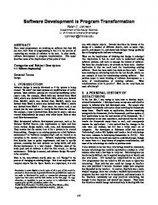
Similar rules are defined for failing computations and free variables as results (see [4]). We illustrate the tracing semantics with a simple example. For the following program the computed trail is depicted in Figure 2. mother x = fcase x of { John -> Christine; Peter -> Monica } father x = fcase x of { Peter -> John } main = let x = x, y = father x in mother y Similarly to the original small-step semantics [1], our tracing semantics is nondeterministic, i.e., it computes a different trail—a graph—for each non-deterministic computation from the initial configuration. In practice, however, it is more convenient to build a single graph that comprises all possible non-deterministic paths (see Section 3.1).
3
Program Transformation
We have implemented a program transformation which converts an arbitrary flat program into an instrumented flat program. This instrumented program writes
0:main
2:mother
3:fcase
9:Christine
4:father
5:fcase
6:Free
8:John
7:Peter
Fig. 2. Trail of a computation.
the trace graph as a side effect at runtime. The basic idea is to wrap all subexpressions of the program with additional function calls. Semantically, these wrapper functions are identities but evaluating them initiates the side effects needed to write the execution trace to a file. 3.1
Path Information
Instead of writing distinct trace graphs for every non-deterministic computation, we generate a unified graph that represents all non-deterministic computations at once. The trace corresponding to one non-deterministic computation can be extracted from the unified graph using path information that is associated with every trace node. Initially, the computation starts with the empty path. Whenever a branching is performed, the subsequent computations are distinguished by extended paths. As an example reconsider the example from above with the call main = let x = x in mother x The unified graph for this example is presented in Figure 3. At each node the path (a list of numbers) is added to the label. This unified graph represents two computations, one with path [1] and the other with path [2]. The two graphs can be computed from the unified graph by considering only nodes with a corresponding path prefix. For instance, the node labeled with 1:[]:mother belongs to both graphs while the node labeled with 6:[1]:Christine only belongs to the graph with path [1]. Generating a unified graph instead of a separate graph for each computation has two advantages. Firstly, large parts of the different graphs are identical (e.g., all nodes labeled with the empty path belong to all graphs). Secondly, in the viewer tool, it is not sufficient to present only a single graph to detect errors related to non-determinism. Rather, different results of a computation have to be presented to the programmer. Furthermore, the information about structures that are identical for two non-deterministic branches can be of great help for debugging, too. It is much easier to obtain these results in the unified graph.
0:[]:main
1:[]:mother
6:[1]:Christine
2:[]:fcase
7:[2]:Monica
4:[1]:John
3:[]:Free
5:[2]:Peter
Fig. 3. Unified trace graph.
Unfortunately, it is not possible to statically determine the order in which non-determinism occurs in the computation, as the following function definition shows: f x y z
= fcase x of { 0 -> fcase y of { 0 -> z }; 1 -> fcase z of { 1 -> 42 }}
The function branches depending on its first argument x: for 0 the function requires the evaluation of y to 0 and returns z; for 1 the function requires the evaluation of its third argument z and yields 42 without initiating the evaluation of y at all. If the evaluation of the arguments y and z introduces non-determinism, then the order in which this non-determinism is introduced into the concrete computation depends on the value for x. The non-determinism in y may not even be introduced at all if x is bound to 1. Hence, the current path has to be propagated at runtime, independently of the evaluation order. In our program transformation, we employ the logic features of Curry to compute the path of a non-deterministic computation. To be able to extend the current path when we perform a non-deterministic branching in or or fcase, we pass the current path as an additional parameter to every function. Initially, this argument is a free variable representing the empty path. Non-empty paths are represented by lists that are terminated by a free variable instead of the empty list (cf. message queues in [8]). Hence, a path is represented as a partially instantiated list of numbers. In contrast to other approaches using advanced list implementations like difference lists in PROLOG or functional lists [10], our lists are not supposed to improve efficiency. They are a means to globally extend paths within non-deterministic computations independently of the evaluation order. The program transformation employs a function extend to extend the path of the current computation. This function is implemented as: extend :: Path -> Int -> a -> a extend p n x | end p =:= (n:ns) = x where ns free
end :: Path -> Path end p = if isVar p then p else end (tail p) We use the auxiliary function end to return the terminating free variable of a path. The function isVar indicates whether the head-normal-form of its argument is a free variable. In order to write a path to a file, we need to replace the free variable that terminates the path with the empty list: path :: Path -> Path path p = if isVar p then [] else head p : path (tail p) 3.2
Labeling Expressions
When writing trace nodes, we need to refer to other nodes in the graph that have not yet been written. For example, to write the node for a function call we need to refer to the function’s arguments. However, these may not have been written into the trace graph yet because of lazy evaluation. In the instrumented semantics we use fresh variable names to refer to unevaluated expressions and use a special operation (x r) to map these variables to node references when the corresponding expression is evaluated. At runtime such variables are not available. Instead, we have to generate similar references and use globally unique labels to represent sub-expressions. New labels are constructed by means of a global state which is accessed by side effects whenever the evaluation of sub-expressions is requested. As a first approach we can think of references as integer values attached to every expression. Every function is transformed accordingly, i.e., it expects labeled values as arguments instead of the original argument values and returns a labeled result. For example, a function of type Bool -> Bool -> Bool would be transformed into a function of type (Int,Bool) -> (Int,Bool) -> (Int,Bool) according to this first approach. Unfortunately, this approach is not sufficient to model compound values. If a component of such a value is selected and passed as argument to some function, we need to be able to determine the label of this sub-term from the original value. In principle, there are two possibilities to store labels for every sub-term of compound values: The first is to provide labeled versions of every datatype and compute with values of this variants instead of the original data-terms. For example, the definition of natural numbers as successor terms data Nat = Z | S Nat can be altered to store labels for each sub-term as follows: data LabeledNat = LZ Int | LS Int LabeledNat Each constructor has an additional argument for the label of the corresponding sub-term. For example, the value (S Z) could be labeled as (LS 1 (LZ 2)). Although this approach is quite intuitive, it also has a severe drawback: It is
not possible to write a Curry function that computes the original value from a labeled value of arbitrary type. We need to compute unlabeled values for two reasons: First, the result of the top-level computation should be presented to the user without labels and, second, external functions must be applied to unlabeled values. Although we can define such un-labeling functions for each particular datatype, this is not sufficient for calls to polymorphic external functions where the current argument-types are unknown. As a solution, we take a different approach: instead of a label, we attach a tree of labels to each expression that represents the labels of all sub-terms of the expression. We define the data-types data Labeled a = Labeled Labels a data Labels = Labels Int [Labels] to model labeled values. The label tree has the same structure as the wrapped data structure. The boolean function mentioned above is transformed into a function of type Labeled Bool -> Labeled Bool -> Labeled Bool and we provide wrapper functions for every defined constructor that operates on labeled values. For example, the wrapper functions for the construction of labeled natural numbers have the following types: z :: Labeled Nat -- Z :: Nat s :: Labeled Nat -> Labeled Nat -- S :: Nat -> Nat Now the value (S Z) is represented as Labeled (Labels 1 [Labels 2 []]) (S Z). With this representation of labeled values it is no problem to define a function value :: Labeled a -> a. Hence, we prefer this solution over the more intuitive approach to label compound values by extending all data types. 3.3
Global State
We provide a library that is imported by every transformed program. This library has two main purposes: a) implement the side effects that write the trace nodes during the computation and b) provide a global state which manages references and labels. At the beginning of each execution trace, the global state must be initialized, i.e. global counters are set to zero, old trace files are deleted and some header information is written to the new trace file. All this is done by initState :: IO (). It is necessary to use a global state instead of passing values through the program, e.g. by a state monad, since tracing must not modify the evaluation order. As already discussed in Section 3.1 the evaluation order is statically unknown. The state cannot be passed and has to be modified by side effects. There are two global counters, one to provide the references, which corresponds to the Ref. column of the tracing semantics, cf. Section 2. The other counter provides labels for arguments which correspond to the variables in the semantics. The counters are accessed by the according IO actions:
currentRefFromState, currentLabelFromState :: IO Int incrementRefCounter, incrementLabelCounter :: IO () In most cases the access to the current counter is directly followed by incrementing the counter. Hence, we provide nextRefFromState, nextLabelFromState :: IO Int which perform those two actions. In addition to the two counters, there is one more global integer value: the current parent reference. This corresponds to the P ar. column of the semantics and is accessed by the functions setParentInState :: Int -> IO () and getParentFromState :: IO Int. Since all tracing has to be done by side effects, all calls to the library functions are wrapped by a call to the function unsafe :: IO a -> a. Therefore, the functions actually called by the transformed programs look like this: nextRef, nextLabel :: Int nextRef = unsafe nextRefFromState nextLabel = unsafe nextLabelFromState As an example for how the global state is used we present the wrapper function for tracing function calls: traceFunc :: Path -> Name -> [Int] -> Labeled a -> Labeled a traceFunc p name args body = unsafe (do l Name -> [Int] -> a -> a writeFunc p name args x = unsafe (do ref a redirect p l x = unsafe (do ref en } = case value x of { ... ci y1 . . . ymi -> let [l1 , . . . , lmi ] = ls , x1 = Labeled l1 y1 , ... xmi = Labeled lmi ymi in traceBranch r τ (ei ); . . .} To reflect pattern matching on the level of the label information as well, we apply the function argLabels to the matched expression. It selects all sub-label-trees of the root-label. These label trees are attached to the corresponding sub-terms of the matched value (y1 , . . . , ymi ). Note the renaming of the pattern variables: xk is renamed to yk and redefined as the corresponding labeled value in each branch of the case-expression. The transformation of flexible case expressions is a bit more complicated but can be implemented with similar techniques. If the case argument evaluates to a constructor rooted term, then the flexible case behaves as a rigid case (select). If the case argument of a flexible case evaluates to a free variable, then this variable is non-deterministically instantiated with the patterns of all branches and the evaluation continues with the right-hand side of the corresponding branches (guess). Both cases can only be distinguished at runtime and have to be reflected in the program transformation. We treat this porblem within the application of traceFCase, which branches in dependence of x reducing to a constructor rooted term (τselect ) or a free variable (τguess ). τ (fcase e of branches) = let v = nextRef, r = nextRef, x = τ (e), ls = argLabels x in traceFCase p r v x (τselect r x ls branches) (τguess v r x ls branches)
0:main
1:(||)
2:fcase
5:False
3:False Fig. 4. Trail of a Projection - Tracing Semantics
τguess v r x ls { cn xmn -> en } = fcase value x of { ... ci y1 . . . ymi -> extend p i (let l1 = nextLabel, . . . , lmi = nextLabel, x1 = Labeled l1 (redirect p l1 y1 ), ... xmi = Labeled lmi (redirect p lmi ymi ) in traceBind p 0 c0i v [l1 , . . . , lmi ] ls (traceBranch r τ (ei ))); . . .} In contrast to the select case, we have to record three additional kinds of information in the trace: the non-deterministic branching (similar to or), the free variable and its bindings. The function traceBind writes trace nodes for the bindings of the free variable, where the free variable is represented by a trace node with reference v and written by the function traceFCase. It also unifies the labels l1 , . . . , lmi with the original argument labels ls of the free variable, which are initially uninstantiated. 3.6
Transforming Projections
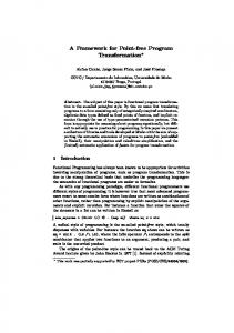
The transformation presented so far reflects the behavior of the tracing semantics with one notable exception: projections. Projections are functions that reduce to one of their arguments, as the following example shows: main = let x = False in x || x (||) :: Bool -> Bool -> Bool x || y = fcase x of { True -> True; False -> y } Tracing the execution of main using the semantics of Section 2 yields the graph shown in Figure 4. When tracing the same program with the transformation introduced so far, the result of the boolean disjunction (||) is not traced. The reason is that if its first argument is False the function (||) is a projection. The tracing semantics adds constructor values to the graph each time they are demanded. The same is not possible with the approach presented so far; values can only be traced when they are demanded for the first time. If a projection is called with a value as argument which has already been evaluated before, then the successor of the projection needs to refer to an already written node.
2:fcase 0:main
5:Proj
1:(||) 3:False Fig. 5. Trail of a Projection - Transformed Program
To solve this problem, we introduce a new kind of trace nodes: projection nodes. Our transformation analyzes the right-hand sides of all defined functions of a program and introduces the special function traceProj that writes a projection node as a side effect. This analysis only checks whether there are defining rules with an argument variable as right-hand side and wraps such variables with a call to traceProj. For example, the transformation of the identity function is: id :: Path -> Labeled a -> Labeled a id p x = traceFunc p "id" [label x] (traceProj p x) With this modification, the above example yields the trace shown in Figure 5. Note, that the resulting graph contains indeed more information than the one of Figure 4: the fact that the value False is also shared in the result of (||). Taking into account the order in which the nodes of the trace graph were written, there exists a simple mapping from the graphs generated by transformed programs to the ones produced by the semantics.
4
Conclusion
We presented a program transformation implementing a tracer for functional logic programs. The transformation exactly reflects a formal tracing semantics defined in previous work except for projections which have to be recorded explicitly. A copying as done in the formal semantics is not possible in the transformed program. However, in the final trace graph projection nodes can be eliminated by copying nodes and we obtain the original, formally defined trace graph. Although our transformation is closely related to the formal semantics it remains to formally prove its equivalence. Our program transformation is implemented for a (slightly different) flat Curry representation used as intermediate language in the Curry implementation PAKCS. Constructing the trace graph by means of the program transformation performs several times faster than our first implementation within a flat Curry interpreter. However, this is not the only advantage of the new approach. Now the trace generation is integrated into the real environment in which systems are developed and arbitrary Curry programs can be traced, independently of new features possibly not available for the interpreter. In contrast our interpreter only supports the core flat Curry language (with only a small set of external functions), but is a good platform for prototypical implementations of semantic based tools.
At the moment we are working on tracing external functions and want to implement a module-wise transformation with a trusting mechanism for selected modules. Furthermore, we are optimizing our viewing tools to cope with nondeterminism and the large size of applications that can now be traced.
References 1. E. Albert, M. Hanus, F. Huch, J. Oliver, and G. Vidal. Operational semantics for declarative multi-paradigm languages. Journal of Symbolic Computation, 40(1):795–829, 2005. 2. S. Antoy and S. Johnson. TeaBag: A functional logic language debugger. In Herbert Kuchen, editor, Proc. of the 13th International Workshop on Functional and (constraint) Logic Programming (WFLP’04), pages 4–18, Aachen, Germany, June 2004. 3. B. Braßel, O. Chitil, M. Hanus, and F. Huch. Observing functional logic computations. In Proc. of the Sixth International Symposium on Practical Aspects of Declarative Languages (PADL’04), pages 193–208. Springer LNCS 3057, 2004. 4. B. Braßel, M. Hanus, F. Huch, and G. Vidal. A semantics for tracing declarative multi-paradigm programs. In Proceedings of the 6th ACM SIGPLAN International Conference on Principles and Practice of Declarative Programming (PPDP’04), pages 179–190. ACM Press, 2004. 5. R. Caballero and M. Rodr´ıguez-Artalejo. DDT: a declarative debugging tool for functional-logic languages. In Proceedings of the 7th International Symposium on Functional and Logic Programming (FLOPS 2004), pages 70–84. Springer LNCS 2998, 2004. 6. O. Chitil, C. Runciman, and M. Wallace. Freja, hat and hood – a comparative evaluation of three systems for tracing and debugging lazy functional programs. In Proc. of the 12th International Workshop on Implementation of Functional Languages (IFL 2000), pages 176–193. Springer LNCS 2011, 2001. 7. Andy Gill. Debugging Haskell by observing intermediate datastructures. Electronic Notes in Theoretical Computer Science, 41(1), 2001. 8. M. Hanus. Distributed Programming in a Multi-Paradigm Declarative Language. In Proc. of the International Conference on Principles and Practice of Declarative Programming (PPDP’99), pages 376–395. Springer LNCS 1702, 1999. 9. M. Hanus (ed.). Curry: An integrated functional logic language. Available at http://www-i2.informatik.rwth-aachen.de/~hanus/curry, 1997. 10. John Hughes. A novel representation of lists and its application to the function ”reverse”. Inf. Process. Lett., 22(3):141–144, 1986. 11. F. L´ opez-Fraguas and J. S´ anchez-Hern´ andez. TOY: A multiparadigm declarative system. In Proc. of RTA’99, pages 244–247. Springer LNCS 1631, 1999. 12. H. Nilsson and J. Sparud. The Evaluation Dependence Tree as a Basis for Lazy Functional Debugging. Automated Software Engineering, 4(2):121–150, 1997. 13. S. Peyton Jones, editor. Haskell 98 Language and Libraries—The Revised Report. Cambridge University Press, 2003. 14. E. Shapiro. Algorithmic Program Debugging. MIT Press, Cambridge, Massachusetts, 1983. 15. J. Sparud and C. Runciman. Tracing Lazy Functional Computations Using Redex Trails. In Proc. of the 9th Int’l Symp. on Programming Languages, Implementations, Logics and Programs (PLILP’97), pages 291–308. Springer LNCS 1292, 1997.