Dec 23, 2008 - He has been helping Eddie and Sam search for quantum algorithms for the last 10 years. SAM GUTMANN crosses the river (from the math ...
T HEORY OF C OMPUTING, Volume 4 (2008), pp. 169–190 http://theoryofcomputing.org
A Quantum Algorithm for the Hamiltonian NAND Tree Edward Farhi
Jeffrey Goldstone
Sam Gutmann
Received: June 6, 2008; published: December 23, 2008.
Abstract: We give a quantum algorithm for the binary NAND tree problem in the Hamiltonian oracle model. √ The algorithm uses a continuous time quantum √ walk with a running time proportional to N. We also show a lower bound of Ω( N) for the NAND tree problem in the Hamiltonian oracle model. ACM Classification: F.1.2, F.2.2 AMS Classification: 68Q10, 68Q17 Key words and phrases: quantum computing, NAND trees, and-or trees, game trees, quantum walk
1
Introduction
The NAND trees in this paper are complete binary trees of depth n, with N = 2n leaves. Each leaf is assigned a value of 0 or 1 and the value of any other node is the NAND of the two connected nodes just above. The goal is to evaluate the value at the root of the tree. An example is shown in Figure 1. Classically, there is a best possible randomized algorithm that succeeds after evaluating only (with high probability) O(N .753 ) of the leaves [10, 11, 12]. As far as we know, no quantum algorithm has been devised√which improves on the classical query complexity. However there is a quantum lower bound of Ω( N) calls to a quantum oracle [2]. In this paper we are not working in the usual quantum query model but rather with a Hamiltonian oracle [6, 8] which encodes the NAND tree instance. We √ evaluates √ will present a quantum algorithm which the NAND tree in a running time proportional to N. We also prove a lower bound of Ω( N) on the running time for any quantum algorithm in the Hamiltonian oracle model. Authors retain copyright to their work and grant Theory of Computing unlimited rights to publish the work electronically and in hard copy. Use of the work is permitted as long as the author(s) and the journal are properly acknowledged. For the detailed copyright statement, see http://theoryofcomputing.org/copyright.html.
c 2008 Edward Farhi, Jeffrey Goldstone, and Sam Gutmann
DOI: 10.4086/toc.2008.v004a008
E DWARD FARHI , J EFFREY G OLDSTONE , AND S AM G UTMANN
Figure 1: A classical NAND tree.
Our quantum algorithm uses a continuous time quantum walk on a graph [7]. We start with a perfectly bifurcating tree of depth n and one additional node for each of the N leaves. To specify the input we connect some of these N pairs of nodes. A connection corresponds to an input value of 1 on a leaf in the classical NAND tree and the absence of a connection corresponds to a 0. See the top of Figure 2. Next we attach a long line of nodes to the root of the tree. We call this long line the “runway.” See the bottom of Figure 2. The Hamiltonian for the continuous time quantum walk we use here is minus the adjacency matrix of the graph. As usual with continuous time quantum walks, nodes in the graph correspond to computational basis states.
Figure 2: The full Hamiltonian HO + HD .
We can decompose this Hamiltonian into an oracle, HO , which is instance dependent and a driver, HD , which is instance independent. HD is minus the adjacency matrix of the perfectly bifurcating tree of depth n whose root is attached to node 0 of the line of nodes running from −M to M. We will take M to be very large. See Figure 3.
Figure 3: The oracle independent driver Hamiltonian HD .
T HEORY OF C OMPUTING, Volume 4 (2008), pp. 169–190
170
A Q UANTUM A LGORITHM FOR THE H AMILTONIAN NAND T REE
HO is minus the adjacency matrix of a graph consisting of the leaves of the bifurcating tree and the parallel set of N other nodes. Each leaf in the tree is connected or not to its corresponding node in the set above. See Figure 4. The quantum problem is: Given the Hamiltonian oracle HO , evaluate the NAND tree with the corresponding input.
Figure 4: The Hamiltonian oracle HO .
Our quantum algorithm evolves with the full Hamiltonian HO + HD , which is minus the adjacency matrix of the full graph illustrated in Figure 2. The initial state is a carefully chosen right-moving packet of length L localized totally on the √ left side of the runway with the right edge of the packet2 at node 0. It will turn out that L is of order N. We take M to be much larger than L, say of order L . We now let the quantum system evolve and wait a time L/2 which is the time it would take this packet to move a distance L to the right if the tree were not present. We then measure the projector onto the subspace corresponding to the right side of the runway. If the quantum state is found on the right we evaluate the NAND tree to be 1 and if the quantum state is not on the right we evaluate the NAND tree to be 0. We have chosen our right-moving packet to be very narrowly peaked in energy around E = 0. (Note that E = 0 is not the ground state but is the middle of the spectrum.) The narrowness of the packet in energy forces the packet to be long. If we did not attach the bifurcating tree at node 0, the packet would just move to the right and we would find it on the right when we measure. The algorithm works because with the tree attached the transmission coefficient at E = 0 is 0 if the NAND tree evaluates to 0 and the transmission coefficient at E = 0 is 1 if the NAND tree √ evaluates to 1. The transmission coefficient is a rapidly changing function of E but for |E| < 1/(γ N), where γ is N-independent and large, the transmission coefficient is not far from its value at E = 0. To guarantee √ that the packet consists mostly √ of energy eigenstates with their energies in this range, we take L to be γ N. This determines the O( N) run time of the algorithm. Our algorithm uses the driver Hamiltonian HD to evaluate the NAND tree. An arbitrary algorithm can add any instance independent HA (t) to HO and work in the associated Hilbert space. We will show that for any choice of instance independent √ HA (t) the running time required to evaluate the NAND tree associated with HO is of order at least N.
2
Motion on the runway
Here we describe the evolution of a quantum state initially localized on the left side of the runway in Figure 2 headed to the right. M is so large that we can take it to be infinite as is justified by the fact that the speed of propagation is bounded. First consider the infinite runway with integers r labeling the sites. The tree is attached at r = 0. We then have for all r not equal to 0: H |ri = −|r + 1i − |r − 1i
r 6= 0 .
T HEORY OF C OMPUTING, Volume 4 (2008), pp. 169–190
(2.1) 171
E DWARD FARHI , J EFFREY G OLDSTONE , AND S AM G UTMANN
For θ > 0, eirθ and e−irθ correspond to the same energy (nonnormalized) eigenstate of equation (2.1) with energy E(θ ) = −2 cos θ but the first is a right-moving wave and the second is a left-moving wave. We are interested in a packet, that is, a spatially finite superposition of energy eigenstates, which is incident from the left on the node 0 and the attached tree. This packet will reflect back and also transmit to the right side of the runway. The packet is dominated by energy eigenstates, |Ei, of the form on the runway (� � eirθ + R(E) e−irθ for r ≤ 0 , hr|Ei = (2.2) irθ T (E)e for r ≥ 0 . (The states |Ei do not vanish in the tree.) There are other energy eigenstates, but we will not need them after the discussion in the next paragraph. Our ultimate aim is to calculate matrix elements hr|e−iHt |si, where r and s label sites on the runway. To this end we need a completeness relation involving all of the energy eigenstates. Standard scattering theory strongly suggest that this will be Zπ
1=
dθ |E(θ )ihE(θ )| + contributions of other eigenstates, 2π
(2.3)
0
i. e., that the way the scattering states are normalized is not changed by the presence of the finite tree scatterer. We now demonstrate this.1 For the sake of brevity we make use of the special properties of our Hamiltonian, though the result is much more general. For the rest of this paragraph only, we relabel the states defined in (2.2) as |E, →i. There are also states, which can be superposed to make left-moving packets, incident on the tree from the right. Now H commutes with the reflection operator, Π, defined by Π|ri = | − ri where r labels a site on the runway Π|ii = |ii
where i labels a site on the tree.
(2.4)
We can obtain the left-moving energy eigenstate |E, ←i by |E, ←i = Π|E, →i ,
(2.5)
( T (E) e−irθ for r 6 0, � hr|E, ←i = � −irθ irθ e + R(E) e for r > 0.
(2.6)
so that on the runway
The states |E, ±i = |E, ←i ± |E, →i are simultaneous eigenstates of H and Π. There might also be a finite set of orthonormal energy eigenstates {|Ek i}, either bound states with hr|Ek i → 0 exponentially as |r| → ∞, or states entirely confined to the tree, i. e., with hr|Ek i = 0 on the runway. Since H and Π are 1 The
reader who is already convinced should skip to the sentence starting above (2.15).
T HEORY OF C OMPUTING, Volume 4 (2008), pp. 169–190
172
A Q UANTUM A LGORITHM FOR THE H AMILTONIAN NAND T REE
commuting self-adjoint operators, the spectral theorem asserts that there are measures f± (θ ) dθ such that Z π
1= 0
f+ (θ ) dθ |E(θ ), +ihE(θ ), +| +
Z π 0
f− (θ ) dθ |E(θ ), −ihE(θ ), −| (2.7)
+ ∑ |Ek ihEk | . k
We are assuming here that the measures are absolutely continuous with respect to Lebesgue measure. In terms of the left and right-moving states (2.7) becomes � � Z π f (θ ) dθ |E(θ ), →ihE(θ ), → | + |E(θ ), ←ihE(θ ), ← | 1= 0 � � Z π (2.8) g(θ ) dθ |E(θ ), →ihE(θ ), ← | + |E(θ ), ←ihE(θ ), → | + 0
+ ∑ |Ek ihEk | . k
We determine f (θ ) and g(θ ) by calculating hr|1|si = δr,s in the two cases r → −∞, s → −∞, with the difference r − s = m fixed, and r → −∞, s → +∞, with r + s = m fixed, making use of the relations |R(E)|2 + |T (E)|2 = 1 R(E)T ∗ (E) + R∗ (E)T (E) = 0 .
(2.9)
These follow from the self-adjointness and reflection symmetry of H, but for our special H can be seen from the explicit expressions for T (E) and R(E) in terms of a real function y(E) that we have in (2.15) and (2.17). With r < 0, s < 0, we find � � Z π i(r−s)θ −i(r−s)θ i(r+s)θ ∗ i(r+s)θ f (θ ) dθ e +e + R(E)e + R (E)e hr|1|si = 0 � � (2.10) Z π g(θ ) dθ T (E)e−i(r+s)θ + T ∗ (E)ei(r+s)θ + ∑ hr|Ek ihEk |si . + 0
k
When r, s → −∞, the integrals linear in R(E) and T (E) go to zero by the Riemann-Lebesgue Lemma, and the terms involving |Ek i also go to zero, so with r − s = m we obtain Z π
2 0
f (θ ) cos m θ dθ = δm,0 .
(2.11)
This determines f (θ ) = 1/2π. With r < 0, s > 0, we find � � Z π f (θ ) dθ T (E)e−i(r−s)θ + T ∗ (E)ei(r−s)θ hr|1|si = 0 � � Z π i(r+s)θ −i(r+s)θ −i(r−s)θ ∗ i(r−s)θ g(θ ) dθ e +e + R(E)e + R (E)e + 0
+ ∑ hr|Ek ihEk |si . (2.12) k
T HEORY OF C OMPUTING, Volume 4 (2008), pp. 169–190
173
E DWARD FARHI , J EFFREY G OLDSTONE , AND S AM G UTMANN
When r → −∞, s → +∞ with r + s = m, we obtain Z π
g(θ ) dθ cos mθ = 0 .
2
(2.13)
0
Thus determines g(θ ) = 0, so that we have the desired completeness relation � � Z 1 π dθ |E, →ihE, → | + |E, ←ihE, ← | + ∑ |Ek ihEk | . 1= 2π 0 k
(2.14)
We will use this completeness relation to prove our results. In particular we will only get relevant contributions from the first term and we go back to (2.2) with the symbol → dropped. Returning to (2.2) and looking at r = 0 we see that 1 + R (E) = T (E) .
(2.15)
The transmission coefficient T (E) is determined by the structure of the tree. In particular let y (E) =
hroot|Ei hr = 0|Ei
(2.16)
where “root” is the node immediately above r = 0 on the runway, see Figure 2. Applying the Hamiltonian at |r = 0i gives H|r = 0i = −|r = −1i − |r = 1i − |rooti and taking the inner product with |Ei gives T (E) =
2 i sin θ . 2 i sin θ + y (E)
(2.17)
In the next section we will show how to calculate y(E) and show that if the NAND tree evaluates to 1 then y(0) = 0 meaning that T (0) = 1 and if the NAND tree evaluates to 0 then y(0) = ∞ and T (0) = 0. Unfortunately we cannot build a state with only E = 0 since it would be infinitely long. Instead we build a finite packet that is long enough so that it is effectively a superposition of the states |Ei with E close enough to 0 that T (E) is close to T (0). We introduce two parameters ε and D for which |T (E) − T (0)| < D|E| for |E| < ε .
(2.18)
The parameters ε and D do depend on the size of the tree, but for the remainder of this section we only use ε � 1. The initial state we consider, |ψ(0)i, is given on the runway as ( √1 eirπ/2 for −L + 1 ≤ r ≤ 0 , L hr|ψ(0)i = (2.19) 0 for r ≤ −L and r > 0 . and vanishes in the tree. For this state hψ(0)|H|ψ(0)i = 0 and hψ(0)|H 2 |ψ(0)i =
5 L
T HEORY OF C OMPUTING, Volume 4 (2008), pp. 169–190
(2.20) 174
A Q UANTUM A LGORITHM FOR THE H AMILTONIAN NAND T REE
√ so the spread in energy about 0 is of order 1/ L. However, for our purpose we will see that this state is effectively more narrowly peaked in energy, and (2.20) is really an artifact of its sharp edge. In fact most of the probability in energy is contained in a peak around 0 of width 1/L. Because we take π/2 and not −π/2 in (2.19) we have a right-moving packet with energies near 0. Evolving with the full Hamiltonian of the graph we have |ψ(t)i = e−iHt |ψ(0)i . We decompose |ψ(t)i into two orthogonal parts, |ψ(t)i = |ψ1 (t)i + |ψ2 (t)i where π
|ψ1 (t)i =
2 +ε Z
dθ −itE(θ ) e |E(θ )i hE(θ )|ψ(0)i 2π
(2.21)
π 2 −ε
and |E(θ )i is given in (2.2) with the completeness relation (2.3). The state |ψ2 (t)i is a superposition of the other eigenstates of H, that is, states incident from the left with 0 < θ < π2 − ε and π2 + ε < θ < π, states incident from the right and bound states with |E| > 2 and hr|Ei → 0 exponentially as r → ±∞ on the runway. We do not need the details of |ψ2 (t)i since we will show in Section 5 that the norm of |ψ1 (t)i is close to 1 so the norm of |ψ2 (t)i is near 0. In other words, |ψ1 (t)i is a very good approximation to |ψ(t)i. To ensure this we need 1 L� . ε We would then expect that at late enough times we will see on the right a packet like the incident packet, but multiplied by T (0) and moving to the right, with the group velocity dE/dθ evaluated at θ = π/2 which is 2. In Section 5 we show, if t is not too big, that for r > 0 hr|ψ(t)i = T (0) hr − 2t|ψ(0)i
(2.22)
plus small corrections. (In Section 5 we also make sense of this equation for 2t not an integer.) To ensure (2.22) we also need L � D2 ε . Since |ψ(0)i is a normalized state localized between r = −L + 1 and r = 0, (2.22) implies that for t > L/2
∑ |hr|ψ(t)i|2 = |T (0)|2
r>0
plus small corrections so the cases T (0) = 1 and T (0) = 0 can be distinguished by a measurement on the right at t > L/2. T HEORY OF C OMPUTING, Volume 4 (2008), pp. 169–190
175
E DWARD FARHI , J EFFREY G OLDSTONE , AND S AM G UTMANN
3
Evaluating the transmission coefficient near E = 0
From the last section, equation (2.17), we see that we can find T (E) if we know y(E). We now show how the structure of the tree recursively determines y(E). Consider the tree in Figure 2 ignoring the runway but including the runway node at r = 0. Except at the top or bottom of this tree every node is connected to two nodes above and one below. See Figure 5 where a, b, c and d are the amplitudes of |Ei at the corresponding nodes.
Figure 5: The amplitudes at 4 nodes in the middle of the tree in an energy eigenstate.
Applying H at the middle node yields: E a = −b − c − d from which we get Y =−
1 E +Y 0 +Y 00
where Y = a/d,Y 0 = b/a and Y 00 = c/a. This is shown pictorially in Figure 6. The y we seek is Y at
Figure 6: The recursion for Y . the bottom of the tree. To find it we recurse down from the top of the tree. At the top of the tree there are 3 possibilities with the respective values of Y obtained by applying the Hamiltonian. The results are shown in Figure 7. From Figures 6 and 7 we see that Y (−E) = −Y (E) so we can restrict attention to E > 0. We now show that the recursive formula for computing the the values Y at E = 0 is in fact the NAND gate. Looking at Figure 7 and taking E → 0 positively we get Figure 8. We see that when we begin our T HEORY OF C OMPUTING, Volume 4 (2008), pp. 169–190
176
A Q UANTUM A LGORITHM FOR THE H AMILTONIAN NAND T REE
Figure 7: The values of Y at the top of tree.
Figure 8: The values of Y at the top of the tree as E → 0+ .
recursion as E → 0+ there are two initial values of Y which are -∞ and 0. Returning to Figure 6 with the different possibilities for Y 0 and Y 00 we get Figure 9. Identifying Y = 0 with the logical value 1 and Y = −∞ with the logical value 0 we see that Figure 9 is a NAND gate. Accordingly the value of y(0) = Y (0) at the bottom of the tree (see (2.16) and Figure 2) is the value of the NAND tree with the input specified at the top.
Figure 9: The recursion for Y at E = 0 implements the NAND gate.
We now move away from E = 0 to see how far from E = 0 we can go and still have the value of the NAND tree encoded in y(E) at the bottom. Near E = 0 it is convenient to write Y (E) either as a(E) E or as −1/(b(E)E) and we will find bounds on how large a(E) and b(E) can become as we move down the tree. We observe that the coefficient of E in Y (E) (here we mean either a(E) or b(E)) on any edge is an increasing function of the coefficients on the two edges above, as long as |aE|, |a0 E|, |bE| and |b0 E| are T HEORY OF C OMPUTING, Volume 4 (2008), pp. 169–190
177
E DWARD FARHI , J EFFREY G OLDSTONE , AND S AM G UTMANN
not too big. To see this use the recursive formula in Figure 6. There are three cases and we obtain figure (10) which makes the increasingness clear.
Figure 10: The coefficient of E in Y is an increasing function of a, a0 , b and b0 .
Now consider a piece of the bifurcating tree as depicted in Figure 11. There are 4 different values of
Figure 11: Y determined by four values of Y above. Y at the top of the piece, which determine Y at the bottom of the piece. Suppose for 0 < E < 2−n/2 /16 each of the Y at the top of the piece obeys 0 ≤ Yi (E) ≤ c E
or
0≤
−1 ≤ cE Yi (E)
for some positive c with c + 1 ≤ 4 · 2 j where j ≤ n/2. We will show 0 ≤ Y (E) ≤ c∗ E where (c∗ + 1) =
or
0≤
−1 ≤ c∗ E Y (E)
2(c + 1) . 1 − 2−n+2 j /4
(3.1)
(3.2)
There are six cases to consider and here we exhibit the most dangerous case; see Figure 12. The reason we can use the coefficient c on the four top edges is the increasingness referred to earlier. Here Y (E) = d(E)E. Using the recursion from Figure 10 we get d(E) =
2c + 1 2c + 1 � � ≤ 2 c 1 − 1 + 1−(1+c)cE (2c + 1)E 2 1 − (1 + 2c)(2c + 1)E 2
T HEORY OF C OMPUTING, Volume 4 (2008), pp. 169–190
178
A Q UANTUM A LGORITHM FOR THE H AMILTONIAN NAND T REE
Figure 12: The most dangerous case.
using (1 + c) ≤ 4 · 2n/2 and E 2 ≤ d(E) ≤
1 162
2−n . So
2(c + 1) 2(c + 1) 2c + 1 ≤ −1 ≤ −1, 2 2 2 2 1 − 4(1 + c) E 1 − 4(1 + c) E 1 − 22 j−n /4
(3.3)
using 1 + c ≤ 4 · 2 j and E ≤ 2−n/2 /16. From (3.3) we get the left side of (3.1) with c∗ given in (3.2). (From Figure 10, the bounds on c and E also imply that the coefficients remain positive from one level to the next, so 0 ≤ Y (E).) The other cases yield smaller coefficients and we will not run through them here. At the top of the full tree Y (E) = E/(1 − E 2 ) or Y (E) = −1/E as can be seen from Figure 7. Given the restriction O < E < 2−n/2 /16 we can take ctop =
1 . 1 − 2−n
(3.4)
Moving down the tree we get after n/2 iterations of (3.2) with j = 1, 2, . . . n/2, �� � � � � � 2 2 2 ∗ ... . (cbottom + 1) = ctop + 1 1 − 22−n /4 1 − 24−n /4 1 − 2n−n /4 Therefore c∗bottom
≤
� 1 + 1−21 −n 2n/2 1−
1 4
n/2 ∑ j=1 22 j−n
≤
� 1 + 1−21 −n 2n/2 1 − 13
(3.5)
≤ 4 · 2n/2
also justifying the assumption c ≤ 4 · 2 j at each step. This means that |y(E)| at √ the bottom is either less than |c∗bottom E| or greater than |1/(c∗bottom E)| for −n/2 |E| < 2 /16. The crucial N arose because the coefficients of Y (E) could barely more than double as we moved two levels down the tree. Going back to the relation between y(E) and the transmission coefficient given in (2.17) we summarize our results for this section: √ 1 1 NAND = 0 (reflect) |y| > 4√N|E| |T | < 8 N|E| for |E| < 16√ N √ √ 1 √ NAND = 1 (transmit) |y| < 4 N|E| |T − 1| < 3 N|E| for |E| < 16 N T HEORY OF C OMPUTING, Volume 4 (2008), pp. 169–190
179
E DWARD FARHI , J EFFREY G OLDSTONE , AND S AM G UTMANN
4
Putting it all together
Here we combine the results of Sections 2 and 3 and state the algorithm. First, the algorithm. Given the Hamiltonian oracle corresponding to an instance of the NAND tree problem we construct the full Hamiltonian HO + HD which is minus the adjacency matrix of the graph in Figure 2. We then build the initial state 0 1 |ψ(0)i = √ eirπ/2 |ri (4.1) ∑ L r=−L+1 where r is on the runway. We choose
√ L=γ N
(4.2)
with γ � 1 a constant independent of N. We let the state evolve for a time trun =
L 2
(4.3)
and then measure the projector P+ onto the right side of the runway M
P+ =
∑ |rihr| .
(4.4)
r=1
If the measurement yields 1 we evaluate the NAND tree to be 1 and if the measurement yields 0 we evaluate the NAND tree to be 0. According to the results stated in Section 2, the probability of getting a measurement result of 1 is very near |T (0)|2 if 1 L� and L � D2 ε . (4.5) ε From the table at the end of Section 3 we can take 1 √ 16 N
(4.6)
√ D=8 N
(4.7)
ε= and
and then the choice� γ � 1 ensures (4.5). At the end of section q �q � 5 we will see that the error probability of � � ε 1/4 1 ε 1 √ the algorithm is O Lε , D L , L which is O γ for large N. By choosing γ large enough we can make the success probability as close to 1 as desired.
5
Technical details
Here we flesh out the claims made in Section 2 and put bounds on the corrections to the stated results. Since we work with θ close to π/2 it is convenient to write θ = ϕ + π/2 T HEORY OF C OMPUTING, Volume 4 (2008), pp. 169–190
180
A Q UANTUM A LGORITHM FOR THE H AMILTONIAN NAND T REE
and E (ϕ + π/2) = 2 sin ϕ so (2.21) becomes |ψ1 (t)i =
Zε −ε
dϕ −2it sin ϕ e |E(ϕ + π/2)ihE(ϕ + π/2)|ψ(0)i 2π
where ε is the small parameter introduced in (2.18). Using (2.2) gives L−1
1 hE(ϕ + π/2)|ψ(0)i = √ L
∑
� irϕ e + (−1)r R∗ (E) e−irϕ .
r=0
We now break |ψ1 (t)i into two pieces |ψ1 (t)i = |ψA (t)i + |ψB (t)i where |ψA (t)i =
Zε −ε
dϕ −2it sin ϕ e A(ϕ)|E(ϕ + π/2)i 2π
with 1 A(ϕ) = √ L and |ψB (t)i =
Zε −ε
with 1 B(ϕ) = √ L
L−1
1
∑ eirϕ = √L
r=0
eiLϕ − 1 eiϕ − 1
(5.1)
(5.2)
dϕ −2it sin ϕ ∗ e R (E) B(ϕ) |E(ϕ + π/2)i 2π L−1
1
∑ (−1)r e−irϕ = √L
r=0
1 − (−1)L e−iLϕ . 1 + e−iϕ
Note that |ψA (t)i and |ψB (t)i are not orthogonal. Now |B(ϕ)|2
ϕ π
dϕ |A(ϕ)|2 + 2π
Zπ
dϕ 1 |A(ϕ)|2 = 2π L
dϕ 1 |A(ϕ)|2 = 2π π
(5.4)
L−1
∑ 1=1
(5.5)
r=0
Zπ
ε
1 dϕ L
sin 12 Lϕ
ε
sin
!2
1 2ϕ
0
Using |ψ(t)i = |ψA (t)i + |ψB (t)i + |ψ2 (t)i T HEORY OF C OMPUTING, Volume 4 (2008), pp. 169–190
182
A Q UANTUM A LGORITHM FOR THE H AMILTONIAN NAND T REE
and the bounds on the norms (5.3), (5.7) and (5.8) we get �
1 � ε �1/4 hψ(t)|P+ |ψ(t)i = hψA (t))|P+ |ψA (t)i + O √ , Lε L
� (5.9)
so we can use |ψA (t)i to estimate the probability of finding the state on the right at time t. Now for r ≥ 0 from (2.2) and (5.1) Zε
hr|ψA (t)i =
dϕ −2it sin ϕ e T (E) A(ϕ) ir eirϕ . 2π
−ε
Let r
Zπ
ar (t) = T (0) i
−π
dϕ i(r−2t)ϕ e A(ϕ) . 2π
(5.10)
We want to show that ar (t) is a good approximation to hr|ψA (t)i. We can write hr|ψA (t)i = ar (t) + br (t) + cr (t) + dr (t)
(5.11)
with br (t) = −ir T (0)
Z−ε dϕ 2π
−π
Zε
r
cr (t) = i T (0) −ε
Zπ
dϕ
ε
2π
+
ei(r−2t)ϕ A(ϕ) ,
dϕ −2it sin ϕ (e − e−2itϕ ) eirϕ A(ϕ) 2π
and r
Zε
dr (t) = i
−ε
dϕ (T (E) − T (0)) e−2it sin ϕ eirϕ A(ϕ) . 2π
We now show that br (t), cr (t) and dr (t) are small. First ∞
2
∑ |br (t)|
r=0
∞
2
2
< ∑ |br (t)| = |T (0)| · 2 · −∞
Zπ
dϕ |A(ϕ)|2 2π
ε
by Parseval’s Theorem. Using (5.6) we have ∞
�
1 ∑ |br (t)| = O Lε r=0 2
� .
T HEORY OF C OMPUTING, Volume 4 (2008), pp. 169–190
(5.12)
183
E DWARD FARHI , J EFFREY G OLDSTONE , AND S AM G UTMANN
Similarly ∞
2
∑ |cr (t)|
2
< |T (0)|
r=0
Zε
2 dϕ 2it(ϕ−sin ϕ) − 1 |A(ϕ)|2 e 2π
−ε Zε 2
(5.13) dϕ 2π
= |T (0)|
−ε
�
� 1 2 6 1 sin2 21 Lϕ t ϕ +··· . 9 L sin2 12 ϕ
However we take trun to be near L/2. As long as Lε 3 � 1 we have ∞
∑ |cr (t)|2 = O(Lε 5 ) .
(5.14)
r=0
To keep this small we need Lε 5 � 1, but this follows from our assumption that Lε 3 � 1 since ε � 1. The assumption that Lε 3 � 1 helps us to establish the translation property in (2.22) which simplifies the picture of what is going on. Also ∞
2
∑ |dr (t)|
r=0
Zε
< −ε
dϕ |T (E) − T (0)|2 |A(ϕ)|2 . 2π
Using |T (E) − T (0)| < D|E| for |E| < ε we get ∞
2
2
∑ |dr (t)|
Zε
< D
r=0
−ε
dϕ 1 sin2 ( 12 Lϕ) 4 sin2 ϕ 2π L sin2 ( 12 ϕ)
D2 ε = O L
(5.15)
�
�
(5.16)
from which we get our condition L � D2 ε . Now from (2.19) and (5.2) we have r
hr|ψ(0)i = i
Zπ
A(ϕ) eirϕ d ϕ .
(5.17)
−π
So from (5.10) we see that ar (t) = T (0) hr − 2t|ψ(0)i
(5.18)
but only when 2t is an integer. However if 2t = m + τ with m an integer and 0 ≤ τ < 1, ∞
∑ |ar (t) − ar
−∞
�m� 2
2
|
2
= |T (0)|
Zπ
−π
dϕ 1 sin2 21 Lϕ iτϕ |e − 1|2 2π L sin2 12 ϕ
� � 1 = O . L T HEORY OF C OMPUTING, Volume 4 (2008), pp. 169–190
(5.19) 184
A Q UANTUM A LGORITHM FOR THE H AMILTONIAN NAND T REE
We have shown that for r > 0, hr|ψ(t)i is well approximated by hr|ψ1 (t)i which is well approximated by hr|ψA (t)i which is well approximated by ar (t) which has the form (5.18) so (2.22) is justified. Furthermore, using (5.9), (5.11), (5.12), (5.14), (5.16) and (5.18) we have for t > L/2 r � � � � ε ε 1/4 1 2 hψ(t)|P+ |ψ(t)i = |T (0)| + O √ , D , (5.20) L L Lε which can be used to estimate the failure probability of the algorithm.
6
A lower bound for the Hamiltonian NAND tree problem via the Hamiltonian Parity problem
Here we show that if the input to a NAND tree problem is given by the Hamiltonian oracle HO described HA (t), evolution using HO + HA (t) cannot evaluate in Section 1 then for an arbitrary driver Hamiltonian √ √ the NAND tree in a time of order less than N. This means that our algorithm which takes time N is optimal up to a constant. √ In the usual query model, the parity problem with N variables can be embedded in a NAND tree with N leaves [2]. To see this first consider 2 variables, a and b, and the 4 leaf NAND tree given in Figure 13 which evaluates to (1 + a + b) mod 2. Using this we see that with 4 variables a, b, c, d the to (1 + a + b + c + d) mod 2. This clearly continues. Since we know NAND tree in Figure 14 evaluates √ √ that the parity problem for N variables cannot be solved with less than of order√ N quantum queries, we know that the NAND tree problem cannot be solved with fewer than of order N quantum queries.
Figure 13: This NAND tree evaluates to (1 + a + b) mod 2.
Figure 14: This NAND tree evaluates to (1 + a + b + c + d) mod 2.
In our Hamiltonian oracle model the input in Figure 14 becomes the oracle depicted in Figure 15. Here the labels on the vertical edges on the top are always 0 or −1. A label 0 means that the edge is T HEORY OF C OMPUTING, Volume 4 (2008), pp. 169–190
185
E DWARD FARHI , J EFFREY G OLDSTONE , AND S AM G UTMANN
not included (just as in Figure 4) and accordingly the corresponding Hamiltonian matrix element is 0. A label −1 means that the edge is there (just as in Figure 4) and the corresponding matrix element of the Hamiltonian oracle is −1.
Figure 15: The Hamiltonian oracle for the NAND tree set up to evaluate (1 + a + b + c + d) mod 2. The coefficients are 0 or −1 corresponding to the edge present or not.
We see that the Hamiltonian parity problem can be embedded in the Hamiltonian NAND tree problem. We did this for the Hamiltonian NAND tree oracle considered in this paper, but it can also be done for the more general Hamiltonian NAND tree oracle described in the Conclusion. We will now prove a lower bound√for the Hamiltonian parity problem, in a general setting (see also [8]), which can be used to obtain a N lower bound for the Hamiltonian NAND tree problem. The oracle for the parity problem is a Hamiltonian of this form: K
HOP =
∑ Hj .
(6.1)
j=1
The H j operate on orthogonal subspaces V j with H j = Pj H j Pj where Pj is the projection onto V j . Furthermore we assume kH j k ≤ 1. For each j there are two possible (a )
operators H j j , a j = 0 or 1. The string a1 , a2 , . . . , aK is the input to the parity problem to be solved. In the Hamiltonian oracle model, an algorithm can use (6.1), but has no other access to the string a. This is the most general form for the parity oracle Hamiltonian that we can imagine and it certainly includes the oracle we used to embed Hamiltonian parity in the Hamiltonian NAND tree. Choose an arbitrary driver Hamiltonian HA (t). Let S be an instance of parity, that is, a subset of 1, 2, . . . , K with a j = 1 iff j is an element of S. Starting in an instance independent state |ψ(0)i we evolve for time T according to the Schr¨odinger equation i
d |ψS (t)i = HS (t)|ψS (t)i dt
using the total Hamiltonian HS (t) HS (t) = g(t) HOP + HA (t) where |g(t)| ≤ 1. With the inclusion of the coefficient g(t) it is clear that the Hamiltonian oracle model includes the quantum query model. Let |ψS (T )i be the state reached at time T . A successful algorithm for parity must have
|ψS (T )i − |ψS0 (T )i ≥ δ T HEORY OF C OMPUTING, Volume 4 (2008), pp. 169–190
186
A Q UANTUM A LGORITHM FOR THE H AMILTONIAN NAND T REE
for some K independent δ > 0 if the parity of S and S0 differ. We now show that this suffices to force T to be of order K. Our approach is an analogue to the analog analogue [6] of the BBBV method [3]. We write S ∼ S0 if S and S0 differ by one element. Summing on (S, S0 ) which differ by one element gives
2
d
0 (t)i |ψ (t)i − |ψ
= ∑ 2 ImhψS (t)| (HS (t) − HS0 (t)) |ψS0 (t)i
S ∑0 S dt S∼S S∼S0 =
∑
2 Im hψS (t)| ± 4 j(S,S0 ) |ψS0 (t)i
S∼S0
� � (1) (0) where j (S, S0 ) is the element by which S and S0 differ, and 4 j = g(t) H j − H j . The + sign means that j(S, S0 ) ∈ S whereas the − sign means that j(S, S0 ) ∈ S0 . Now we have
2 d
0 0 0 0 0 ≤ 2 hψ (t)|P 4 P |ψ (t)i |ψ (t)i − |ψ (t)i
S S S S j(S,S ) j(S,S ) j(S,S ) ∑0 ∑0 dt S∼S S∼S
≤ 4 ∑ Pj(S,S0 ) |ψS (t)i · Pj(S,S0 ) |ψS0 (t)i S∼S0
since k4 j k ≤ 2. Using ab ≤
1 2 1 2 2a +2b
�
gives
2 d
0 |ψ (t)i − |ψ (t)i
≤2 ∑ S ∑0 S dt S∼S S∼S0
�
2
2 �
Pj(S,S0 ) |ψS (t)i + Pj(S,S0 ) |ψS0 (t)i .
For fixed S0 , j(S, S0 ) runs over {1, 2, . . . , K} so
∑
S∼S0 ,S0 fixed
2
0 0 |ψ (t)i P
≤1
j(S,S ) S
and similarly for fixed S and thus we have �
2
2 �
∑ Pj(S,S0 ) |ψS (t)i + Pj(S,S0 ) |ψS0 (t)i ≤ 2 · 2K S∼S0
since there 2K possibilities for S0 (or S). We’ve shown that
2 d
|ψS (t)i − |ψS0 (t)i ≤ 4 · 2K , ∑ dt S∼S0 and since
2
0 |ψ (0)i − |ψ (0)i
=0 S ∑ S
S∼S0
we can integrate to obtain
2
0 |ψ (T )i − |ψ (T )i
≤ 4 · 2K · T . S ∑ S
S∼S0
T HEORY OF C OMPUTING, Volume 4 (2008), pp. 169–190
187
E DWARD FARHI , J EFFREY G OLDSTONE , AND S AM G UTMANN
For each S0 there are K choices of S, so a successful algorithm requires
2
0 (T )i |ψ (T )i − |ψ
≥ 2K · K · δ
S ∑ S
S∼S0
and we have the desired bound T ≥ K δ /4 .
Conclusion We are not working in the quantum query model but rather in the quantum Hamiltonian oracle model. In this model the programmer is given a Hamiltonian oracle of the form N
HO =
∑ Hj
j=1
(b )
where the H j operate in orthogonal subspaces. Each H j is one of two possible operators H j j with b j = 0 or 1 and the string b1 · · · bN is the input to the classical NAND tree that is to be evaluated. The quantum programmer is allowed to evolve states using any Hamiltonian of the form g(t) HO + HA (t) where the coefficient g(t) satisfies |g(t)| ≤ 1 and HA (t) is any instance independent Hamiltonian. The programmer has no other access to the string b. The algorithm presented in this paper uses a time independent HO + HD which is (minus) the adjacency matrix of a graph, √ so our algorithm is a continuous time quantum walk. We evaluate the NAND tree in time of order N which is (up to a constant) the lower bound for this problem. After the arXiv version of this paper appeared, corresponding results in the discrete-query model were obtained [1, 4]. Further generalizations to other formulas can be found in [5, 9].
Acknowledgement Two of the authors gratefully acknowledge support from the National Security Agency (NSA) and the Disruptive Technology Office (DTO) under Army Research Office (ARO) contract W911NF-04-1-0216. We also thank Richard Cleve for repeatedly encouraging us to connect continuous time quantum walks with NAND trees, and for discussions about the Hamiltonian oracle model. We thank Andrew Landahl for earlier discussions of the NAND tree problem.
References [1] * A NDRIS A MBAINIS , A NDREW M. C HILDS , B EN W. R EICHARDT, ROBERT Sˇ PALEK , AND S HENGYU Z HANG: Any AND-OR formula of size N can be evaluated in time n1/2+o(1) on a quantum computer. In Proc. 48th FOCS, pp. 363–372. IEEE Computer Society, 2007. [doi:10.1109/FOCS.2007.57]. 6 T HEORY OF C OMPUTING, Volume 4 (2008), pp. 169–190
188
A Q UANTUM A LGORITHM FOR THE H AMILTONIAN NAND T REE
[2] * H OWARD BARNUM AND M ICHAEL S AKS: A lower bound on the quantum query complexity of read-once functions. J. Comput. System Sci., 69(2):244–258, 2004. [doi:10.1016/j.jcss.2004.02.002]. 1, 6 [3] * C HARLES H. B ENNETT, E THAN B ERNSTEIN , G ILLES B RASSARD , AND U MESH VAZIRANI: Strengths and weaknesses of quantum computing. SIAM J. Comput., 26(5):1510–1523, 1997. [doi:10.1137/S0097539796300933]. 6 [4] * A NDREW M. C HILDS , R ICHARD C LEVE , S TEPHEN P. J ORDAN , AND DAVID Y EUNG: Discrete-query quantum algorithm for NAND trees, 2007. [arXiv:quant-ph/0702160]. 6 [5] * R ICHARD C LEVE , D MITRY G AVINSKY, AND DAVID L. Y EUNG: Quantum algorithms for evaluating MIN-MAX trees, 2007. [arXiv:0710.5794]. 6 [6] * E DWARD FARHI AND S AM G UTMANN: An analog analogue of a digital quantum computation. Phys. Rev. A, 57:2403, 1998. [doi:10.1103/PhysRevA.57.2403]. 1, 6 [7] * E DWARD FARHI AND S AM G UTMANN: Quantum computation and decision trees. Phys. Rev. A, 58:915, 1998. [doi:10.1103/PhysRevA.58.915]. 1 [8] * C ARLOS M OCHON: Hamiltonian oracles. [doi:10.1103/PhysRevA.75.042313]. 1, 6
Phys. Rev. A, 75:042313,
2007.
[9] * B EN W. R EICHARDT AND ROBERT Sˇ PALEK: Span-program-based quantum algorithm for evaluating formulas. In Proc. 40th STOC, pp. 103–112. ACM, 2008. [doi:10.1145/1374376.1374394]. 6 [10] * M ICHAEL S AKS AND AVI W IGDERSON: Probabilistic boolean trees and the complexity of evaluating game trees. In Proc. 27th FOCS, pp. 29–38. IEEE Computer Society, 1986. 1 [11] * M IKLOS S ANTHA: On the Monte Carlo Boolean decision tree complexity of read-once formulae. Random Structures Algorithms, 6(1):75–87, 1995. [doi:10.1002/rsa.3240060108]. 1 [12] * M ARC S NIR: Lower bounds on probabilistic decision trees. Theoret. Comput. Sci., 38:69–82, 1985. [doi:10.1016/0304-3975(85)90210-5]. 1
AUTHORS Edward Farhi [About the author] Cecil and Ida Green Professor of Physics Massachusetts Institute of Technology Cambridge, MA 02139 farhi mit edu http://web.mit.edu/physics/facultyandstaff/faculty/edward farhi.html
T HEORY OF C OMPUTING, Volume 4 (2008), pp. 169–190
189
E DWARD FARHI , J EFFREY G OLDSTONE , AND S AM G UTMANN
Jeffrey Goldstone [About the author] Cecil and Ida Green Professor of Physics, Emeritus Massachusetts Institute of Technology Cambridge, MA 02139 goldston mit edu http://web.mit.edu/physics/facultyandstaff/faculty/jeffrey goldstone.html
Sam Gutmann [About the author] Department of Mathematics Northeastern University, Boston MA sgutm neu edu http://www.math.neu.edu/∼Gutmann/
ABOUT THE AUTHORS E DWARD FARHI is a professor of physics and the director of the Center for Theoretical Physics at MIT. He is a lapsed particle physicist hoping to return to his roots when data from experiments offers new insight into how the world really works. Meanwhile he works on quantum computation, primarily focusing on algorithm design. He started collaborating with Sam in high school and with Jeffrey at MIT. J EFFREY G OLDSTONE, after 25 years at Cambridge University and 30 at MIT, is now Professor of Physics Emeritus. He worked on many-body theory and in the prehistoric eras of the standard model and string theory. He has been helping Eddie and Sam search for quantum algorithms for the last 10 years.
S AM G UTMANN crosses the river (from the math department at Northeastern University) to work with Eddie and Jeffrey.
T HEORY OF C OMPUTING, Volume 4 (2008), pp. 169–190
190