A Run-Time Dynamic Reconfigurable Computing ... - Semantic Scholar

energies Article

A Run-Time Dynamic Reconfigurable Computing System for Lithium-Ion Battery Prognosis Shaojun Wang 1,2 , Datong Liu 1, *, Jianbao Zhou 1 , Bin Zhang 3 and Yu Peng 1 1 2 3

*

Department of Automatic Test and Control, Harbin Institute of Technology, Harbin 150080, China; [email protected] (S.W.); [email protected] (J.Z.); [email protected] (Y.P.) Department of Computing, Imperial College London, London SW7 2BZ, UK College of Engineering and Computing, University of South Carolina, Columbia, SC 29208, USA; [email protected] Correspondence: [email protected]; Tel.: +86-451-8641-3533 (ext. 514)

Academic Editor: Shengshui Zhang Received: 21 May 2016; Accepted: 15 July 2016; Published: 25 July 2016

Abstract: As safety and reliability critical components, lithium-ion batteries always require real-time diagnosis and prognosis. This often involves a large amount of computation, which makes diagnosis and prognosis difficult to implement, especially in embedded or mobile applications. To address this issue, this paper proposes a run-time Reconfigurable Computing (RC) system on Field Programmable Gate Array (FPGA) for Relevance Vector Machine (RVM) to realize real-time Remaining Useful Life (RUL) estimation. The system leverages state-of-the-art run-time dynamic partial reconfiguration technology and customized computing circuits to balance the hardware occupation and computing efficiency. Optimal hardware resource consumption is achieved by partitioning the RVM algorithm according to a multi-objective optimization. Moreover, pipelined and parallel computation circuits for kernel function and matrix inverse are proposed on FPGA to further accelerate the computation. Experimental results with two different battery data sets show that, without sacrificing the RUL prediction performance, the embedded RC platform significantly reduces the computation time and the requirement of hardware resources. This demonstrates that complex prognostic tasks can be implemented and deployed on the proposed system, and it can be extended to the embedded computation of other machine learning algorithms. Keywords: field programmable gate array; relevance vector machine; lithium-ion battery; remaining useful life

1. Introduction Lithium-ion batteries are widely used in electric vehicles (EVs), consumer electronics, communications, and aerospace technologies [1], due to their advantages of high energy density, long cycle life and low self-discharge rate [2]. As safety and reliability critical components, lithium-ion batteries and their management, diagnosis and prognosis of state-of-charge (SOC), and state-of-health (SOH), have attracted more and more research efforts in the past decades [3–5]. Particularly, the research on battery capacity degradation and remaining useful life (RUL) estimation are of great interest to battery management system (BMS), prognostics and health management (PHM), reliability engineering, and system design, among many other related areas [3]. From a system design point of view, the estimation of the remaining cycle life and assessment of the health state can be used for control reconfiguration and mission replanning to minimize mission failure risk, improve the system availability, and reduce life-cycle cost [6]. With this understanding, the diagnosis (identification of the current battery SOC and SOH) and prognosis (estimation of the RUL in terms of operation time for

Energies 2016, 9, 572; doi:10.3390/en9080572

www.mdpi.com/journal/energies

Energies 2016, 9, 572

2 of 19

SOC and RUL in terms of charge-discharge cycles for SOH) of lithium-ion battery is considered one of the most valuable issues in electronic PHM [7,8]. To achieve the battery RUL prediction, lots of computational intelligence and machine learning based data-driven approaches, such as autoregressive model [9], artificial neural network [10], and support vector machine [11], have been used. However, most of these methods do not have uncertainty management capability. More important, the RUL prediction focuses on not only the accuracy, but also the precision. The representation and quantification of uncertainty is necessary to the diagnosis and prognosis for decision-making. In uncertainty management of RUL, most applicable approaches are in the Bayesian estimation framework. Typical approaches include Kalman filter, particle filter (PF) [7,8] and their variants [12,13]. The main limitation in these methods is that they rely on a simplified battery degradation model, which is often insufficient in dealing with high nonlinearity and varying operating conditions of batteries. To address this limitation, the emerging Relevance Vector Machine (RVM) is employed in this research for RUL estimation. The RVM is developed with sparse Bayesian learning and kernel learning [14,15] and has shown great potentials in diagnosis and prognosis [15]. With capabilities of uncertainty management and promising results on diagnosis and prognosis, however, RVM is not yet well investigated in the prognostics and health management, especially in RUL estimation and its implementation on hardware, i.e., embedded systems and microprocessors. Most lithium-ion battery RUL estimations are currently implemented on PC platforms. In future intelligent BMSs, it is crucial to design and implement battery prognosis on embedded systems, which are extensively used in industries including EVs and aircrafts. Since embedded systems are often featured by limited computation and storage capability while RUL estimation is a computation intensive problem that usually involves large amount of computation, RUL prognosis on embedded systems brings a significant challenge and this requires efficient embedded computing system being developed. Reconfigurable Computing (RC) is an emerging computing paradigm with the development of FPGA. The innovative feature of RC is that the computation architecture can be modified in runtime to realize high efficient customized and parallel computing. With characteristics of powerful computing resources, small size, low power consumption, and high reliability, FPGA has become a promising trend in high performance computing [16]. FPGA accelerators for multi-class SVM [17], wavelet transform, Fourier transform [18] and other algorithms [19] have been successfully applied in bearing fault diagnosis, induction motor fault detection, and so on. It is worth noting that dynamic run-time reconfiguration feature of modern state-of-the-art FPGAs makes it even more suitable for compact embedded computation intensive applications by time division multiplexing of the hardware [20–22]. However, to our knowledge, all the existing prognosis or diagnosis FPGA accelerators are just FPGA-based customized computing circuits, and none of them focuses on state-of-the-art dynamic run-time reconfiguration ability which can further improve the performance of BMS and make the system volume more compact. This motivates our research in this work. Our research focuses on the lithium-ion battery RUL estimation with a RVM algorithm implemented on a novel FPGA-based dynamic reconfigurable computing architecture. The main contributions include: (1) a FPGA embedded system with dynamic run-time reconfigurable architecture for complex machine learning algorithm; (2) multi-level pipelined and parallel circuits for kernel function and matrix inversion computation; and (3) experimental verification of the proposed algorithm and its implementation on a Virtex-5 FPGA embedded system with NASA and Center for Advanced Life Cycle Engineering (CALCE) lithium-ion battery data sets. It is worth mentioning that the research work presented here is the first work of implementing run-time RC on dynamic reconfigurable FPGA for RVM-based real-time RUL estimation. Different from our previous work [23], this work mainly focuses on the utilization of state-of-the-art run-time reconfigurable feature of FPGA instead of system-on-chip based design. This paper is organized as follows: Section 2 describes the BMS with dynamic reconfigurable computing system. Section 3 introduces the prediction model, RVM and its training algorithm.

Energies 2016, 9, 572

3 of 19

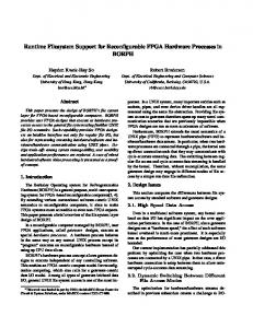
Section 4 describes the RC system for RVM implementation. Section 5 presents experimental results to demonstrate the effectiveness of the proposed FPGA-based RC platform, which is followed by concluding remarks and future works in Section 6. Energies 2016, 9, 572  3 of 18  2. BMS Based on Dynamic Reconfigurable Computing System 2. BMS Based on Dynamic Reconfigurable Computing System  In future intelligent BMSs, diagnosis and prognosis on Li-ion batteries are required to extend the In future intelligent BMSs, diagnosis and prognosis on Li‐ion batteries are required to extend  batteries’ life and ensure the safety and reliability of the systems. However, accurate diagnosis and the batteries’ life and ensure the safety and reliability of the systems. However, accurate diagnosis  prognosis both involve very complicated algorithms, i.e., statistical machine learning, stochastic process. and prognosis both involve very complicated algorithms, i.e., statistical machine learning, stochastic  Moreover, these algorithms should be implemented on embedded computing systems with strict process. Moreover, these algorithms should be implemented on embedded computing systems with  area power consumption constraints for actual applications, such as EVs, strict and area  and  power  consumption  constraints  for industrial actual  industrial  applications,  such satellites. as  EVs,  To meet these requirements, a BMS architecture is described with FPGA based dynamic reconfigurable satellites. To meet these requirements, a BMS architecture is described with FPGA based dynamic  computing system as shown in Figure 1. reconfigurable computing system as shown in Figure 1. 

BMS

Dynamic Reconfigurable Partititon

FPGA Status Sampling Unit

Data Memory Embedded Processor

Li-ion Batteries Charge/Discharge Control Circuits

On Chip Bus

SOC Identification SOH Identification SOC Estimation SOH Estimation

  Figure 1. BMS based on dynamic reconfigurable computing system.  Figure 1. BMS based on dynamic reconfigurable computing system.

As  shown  in  Figure  1,  besides  the  sampling  and  control  circuits  units,  the  FPGA  is  the  main  As shown in Figure 1, besides the sampling and control circuits units, the FPGA is the main control  and  computing  unit  in  BMS.  To  accommodate  those  complex  models  and  algorithms,  control and computing unit in BMS. To accommodate those complex models and algorithms, traditional embedded processor, such as microprocessor, cannot operate efficiently or  are unable to traditional embedded processor, such as microprocessor, cannot operate efficiently or are unable meet performance requirements. To make the BMS more compact and power efficient, complicated  to meet performance requirements. To make the BMS more compact and power efficient, complicated diagnosis and prognosis computations, such as SOC/SOH identification, SOC/SOH estimation, are  diagnosis and prognosis computations, such as SOC/SOH identification, SOC/SOH estimation, realized in  time  division multiplexing mode  in  the dynamic  reconfigurable  partition  of  FPGA.  To  are realized in time division multiplexing mode in the dynamic reconfigurable partition of FPGA. reach high performance under limited hardware resources, customized computing architectures for  To reach high performance under limited hardware resources, customized computing architectures for each diagnosis and prognosis algorithm should be designed.  each diagnosis and prognosis algorithm should be designed. In this work, prognosis, which usually involves RUL estimation of SOH, is chosen as an example  In this work, prognosis, which usually involves RUL estimation of SOH, is chosen as an example to demonstrate how the algorithms are realized in the BMS as shown in Figure 1. The aforementioned  to demonstrate how the algorithms are realized in the BMS as shown in Figure 1. The aforementioned RVM algorithm with capabilities of uncertainty management and promising results on prognosis is  RVM algorithm with capabilities of uncertainty management and promising results on prognosis is selected to show how its customized computing architecture is built. Thus, the basic principle of RVM  selected to show how its customized computing architecture is built. Thus, the basic principle of RVM algorithm as well as its implementation for RUL estimation will be introduced in Part 3. Moreover,  algorithm as well as its implementation for RUL estimation will be introduced in Part 3. Moreover, on a compact FPGA chips, to support multiple algorithms and realize complicated calculations, the  on a compact FPGA chips, to support multiple algorithms and realize complicated calculations, the key key technology is to design the architecture and reconfigurable framework, which will be described  technology is to design the architecture and reconfigurable framework, which will be described in in Part 4.  Part 4. 3. Battery RUL Estimation with RVM Algorithm  3. Battery RUL Estimation with RVM Algorithm 3.1. RVM Algorithm  3.1. RVM Algorithm N Given battery monitoring dataset  ,  x  R ll ,  t  R , the regressive model is:    { x,i ,ttiu}N 1 , x Given battery monitoring dataset tx i i ii“ 1 ii P R , ti i P R, the regressive model is:

t  y (x)     (1) t “ ypxq ` ε (1) N where x is  { x i } i  1 and represents the battery capacity, N is the number of samples,  t   represents the  objective health indicators to show the health state, such as remaining rechargeable cycles;  y ( )   is a  2 nonlinear function, and     is independent additive noise term subject to   ~ N (0,  ) [14]. The RVM  model is as follows: 

t  Φw  ε

(2)

Energies 2016, 9, 572

4 of 19

where x is txi uiN“1 and represents the battery capacity, N is the number of samples, t represents the objective health indicators to show the health state, such as remaining rechargeable cycles; yp¨q is a nonlinear function, and ε is independent additive noise term subject to ε „ Np0, σ2 q [14]. The RVM model is as follows: t “ Φw ` ε (2) where Φ “ rφpx1 q, φpx2 q ¨ ¨¨, φpx N qsT is the kernel function matrix in which φpxi q “ r1, Kpxi , x1 q, ¨ ¨ ¨, Kpxi , x N qs and Kp¨q is the kernel function, w “ pω0 , ¨ ¨ ¨, ω N qT is the weight of the model. Following Bayesian inference, ppti |x q meets ppti |x q „ Npti |ypxq, σ2 q which is a normal distribution of ti with mean ypxq and variance σ2 . The likelihood of the complete data set under the independence assumption of ti can be written as: #

2 ´ N {2

2

ppt|w, σ q “ p2πσ q

||t ´ Φw||2 exp ´ 2σ2

+ (3)

Define a prior zero-mean Gaussian distribution over w: ppw|αq “

N ź ω2 α αi 1{2 ? expp´ i i q 2 2π i “0

(4)

with α “ tα0 , α1 , ¨ ¨ ¨, α N u being a vector of N ` 1 hyper-parameters. The posterior distribution over the weights is thus given by: # 2

ppw|t, α, σ q “ p2πq

´ N`1 2

|Σ|

´1{2

exp ´

pw ´ µqT

ř´1

pw ´ µq

2

+ (5)

where the posterior covariance and mean are: ÿ

´1

“ pσ´2 ΦT Φ ` Aq µ “ σ ´2

ÿ

ΦT t

(6) (7)

and A “ diagpα0 , α1 , ¨ ¨ ¨, α N q. In practice, the posterior distributions of many weights are sharply (indeed infinitely) peaked around zero. These vectors associated with remaining non-zero weights are called Relevance Vectors (RVs). To maximize the posterior probability with the given data, the following distribution of hyper-parameters needs to be maximized: 2

´ N {2

ppt|α, σ q “ p2πq

|C|

´1{2

" * 1 T ´1 exp ´ t pCq t „ Np0, Cq 2

(8)

where C “ σ2 I ` ΦA´1 ΦT . Let the derivative of Equation (8) equal to zero, it leads to [15]: αinew “

γi µ2i

(9)

ř ř where µi is the ith posterior mean weight and γi “ 1 ´ αi ii with ii being the ith diagonal element of the posterior weight covariance computed with the current values of α and σ2 .

Energies 2016, 9, 572

5 of 19

Similarly, the noise variance σ2 can be obtained as: pσ2 q

new

“

||t ´ Φµ|| ř N ´ γi

(10)

i

Given a new test point x˚ , predictions are made for the corresponding target t˚ . Specifically, ř 2 ` φpx qT the distribution of t˚ is ppt˚ |tq „ Npµ˚ , σ˚2 q, where µ˚ “ µT φpx˚ q and σ˚2 “ σMP φpx˚ q ˚ 2 is obtained by maximizing the are the predicted mean and variance of x˚ , respectively, in which σMP updated distribution. 3.2. Expectation Maximization (EM) Algorithm In this work, EM algorithm is used for RVM training [14,15] because it avoids the computing of hyper-parameters. The EM iterative algorithm consists of E-Step (expectation calculation) and M-Step (maximization), as follows: Step 1: Initialization. p1q

Initialize the weight wp1q and variance pσ2 q Step 2: E-step. With wpkq and pσ´2 q

pk q

#

where

Ψpk q

.

at iteration k, estimate wpk`1q at iteration k+1 and EpwwT q

ř pk q wpk`1q “ pσ´2 q pΨpkq ´ Ψpkq ΦT ´1 ΦΨpkq qΦT t ř Ep w wT q “ pΨpkq ´ Ψpkq ΦT ´1 ΦΨpkq q ` w wT

(11)

„ˇ ˇ ˇ ˇ ˇ ˇ  ř ˇ p k q ˇ2 ˇ p k q ˇ2 ˇ p k q ˇ2 “ diag ˇω0 ˇ , ˇω1 ˇ , ¨ ¨ ¨ , ˇω N ˇ and “ ΦΨpkq ΦT ` pσ2 qI.

Step 3: M-step. With wpk`1q , compute the variance pσ2 q pσ2 q

k `1

k `1

as, T

“

tT t ´ 2tT Φ ¨ p wpk`1q q ` tracerΦEpwwT qΦT s N

(12)

where tracep¨q is the trace of the matrix. Step 4: Convergence determination. If ||wpk`1q ´ wpkq ||{||wpkq || ă δ or the algorithm reaches the maximum iteration number, the iteration terminates. Otherwise, go to Step 2 and repeat EM iteration. 4. Run-Time Dynamic Reconfigurable Computing Platform for Embedded RVM Implementation Due to battery’s varying operating conditions and nonlinearity of degradation, dynamic training is always required to improve the RUL prediction performance with the cost of more computation. In this Section, run-time RC computation architecture is proposed by analyzing the computation processes and features of RVM with EM algorithm. The partition of computing tasks is realized by a multi-objective optimization based on dynamic reconfigurable RVM. Parallel computing, pipelining and time-multiplexing techniques are employed to optimize the hardware resources and improve the computation efficiency for embedded systems. 4.1. Computing Process Analysis of RVM Algorithm The computing process of RVM algorithm is mainly composed of Equations (11) and (12). In Equation (11), Φ is a n-dimension kernel function matrix, ΦT t is matrix-vector multiplication, so Φ and ΦT t are determined by training samples and will keep constant during the iteration; ΦΨpkq involves matrix multiplication in each iteration, and Ψpkq ΦT is the transpose matrix of ΦΨpkq ;

Energies 2016, 9, 572

6 of 19

ř and ΦT ´1 Φ involves several matrix multiplication because matrix inversion is needed in the ř calculation of ; and wwT is a n ˆ n matrix. In Equation (12), tT t is a n-dimension vector inner product determined by training samples and keeps unchanged in the iteration; tT Φ is the transpose matrix of ΦT t, which can be obtained

ř

T

from the E-Step directly; tracerΦ EpwwT qΦT s involves matrix multiplication; and tT Φpwpk`1q q is a n-dimension vector inner product. In Equation (12), Φpx˚ q is a n-dimension kernel function vector and wT Φpx˚ q is a vector inner product. Equation (10) is mainly composed of matrix vector multiplications. The above analyses of the computation load show that: ‚

‚

The entire computation process is composed of matrix multiplication, matrix inversion, and kernel function calculation, which involves a lot of computation in the iteration. This indicates that the RVM algorithm is of high complexity and of intensive computation. The training efficiency is determined by the number of iterations, which depends on the training samples and the convergence conditions. Therefore, a well-designed computing architecture is imperative to maximize the utilization of hardware resources and efficiency of RVM.

4.2. Dynamic Reconfigurable RVM RC has two modes: static RC and dynamic RC [24]. Static RC configures the FPGA beforehand and keeps this configuration unchanged in the implementation. It is clear that more FPGA chips are needed to accommodate the high complexity of RVM algorithm in static RC mode and this will increase volume, weight, and power consumption. Moreover, the static mode is not suitable for the multiple algorithms fusion and dynamic algorithm update. Dynamic RC allows FPGAs to be configured partially while other parts of the FPGA are still working. With this time multiplexing feature, large and complex computation tasks can be divided into multiple simple sub-tasks and executed with limited resources. This is more suitable for compact embedded BMS application. In this work, dynamic RC is selected to implement the RVM- based prediction algorithm. In dynamic RC, task partitioning is the key to ensure load balance and computing efficiency. In the dynamic reconfigurable RVM, the simplest way is to manually partition the task into E-Step part and M-Step part according to Figure 1. However, this partition needs to reconfigure the FPGA twice in every iteration of E-step and M-step and this will reduce the computation efficiency. In addition, E-step and M-step involve different sub-tasks that require different hardware resources. It will lead to unbalanced partition and hardware resource waste if these two different tasks are accommodated in one reconfigurable partition. For this reason, optimal computing task partition is critical and needs to be developed. 4.3. Computing Task Partition of Dynamic Reconfigurable RVM An optimal dynamic RC task partition should take into consideration those factors that affect the computing efficiency, such as execution time, number of reconfiguration, size of reconfigurable partitions, and sub-tasks parallelism. Execution time depends on computing delay of the task with given computing resources. Number of reconfiguration must be minimized to increase the efficiency. Each sub-task occupies approximately equal hardware resources to ensure the balance of reconfigurable partitions and decrease the resources consumption. Parallel computing and pipeline computing are utilized to further improve the computational efficiency. In this work, a multi-objective optimization is employed to realize the dynamic RC task partition. In the optimization, the following issues are taken into consideration: Objective task model: The objective task model G is defined as , in which W is the computing time in each reconfigurable partition, V is reconfiguration time, and D is the hardware resources in the reconfigurable partition.

Energies 2016, 9, 572

7 of 19

RVM computation: For a RVM computing task divided into N sub-tasks denoted by P “ tP1 , P2 , ¨ ¨ ¨ , PN u, each sub-task is executed by a reconfigurable partition in time multiplexing mode. The RVM computing is terminated if all the sub-tasks are executed. Subtask execution time: The executing time Xi of sub-task Pi is given by, Xi “ miadd ¨ rd add ` misub ¨ rdsub ` mimul ¨ rdmul ` midiv ¨ rddiv

(13)

where miadd , misub , mimul , and midiv are the numbers of Adders, Subtractors, Multipliers and Dividers in task Pi , while rd add , rdsub , rdmul , and rddiv are the computing delays of the Adders, Subtractors, Multipliers and Dividers in task Pi , respectively. The number of each operator is the sum of the corresponding number of operator in each configuration. These numbers can be obtained by analysis of computation in the task. For specific FPGA and corresponding intellectual property (IP) cores, rd add , rdsub , rdmul , and rddiv are known before partitioning. Configuration time: The configuration time of each task depends on the amount of hardware resources in the reconfigurable partition. In other words, the configuration time Yi for tasks Pi is proportional to the hardware scale in the designated reconfigurable partitions RpPq, and the number of reconfigurations mi for task Pi , which is given as: Yi “ k ¨ RpPq ¨ mi

(14)

where k is a gain. Optimization constraints: For the optimization problem, the following constraints need to be considered: (a)

Dynamic reconfigurable partitions RpPq must be less than the actual FPGA resources, i.e., RpPq ď Rtotal , where Rtotal is the actual FPGA resources. In our applications, 50% of FPGA hardware resources are reserved for algorithm fusion and parallel computing. With this consideration, the dynamic reconfigurable resources is limited by: RpPq ď 0.5Rtotal

(15)

(b)

Resources for each sub-task must be less than the amount of resources in dynamic reconfigurable partitions, namely: RpPi q ď RpPq, i “ 1, 2, ¨ ¨ ¨ , N (16)

(c)

Because different tasks may share the same reconfigurable partition in time multiplexed mode, the resource occupation of each task needs to be balanced to avoid waste of hardware resource. These resources include Look-Up-Table (LUT), block RAM (BRAM), connection resources, and DSP48E resources. DSP48E is the processing unit for a variety of arithmetic computing, such as addition, subtraction, multiplication, and division in FPGA. Since DSP48E resources are the key factors that affect the computing capability of FPGA, to simplify the problem, we keep the balance of DSP48E resource as follows: RpPiE q ´ RpPjE q ď ∆, i ‰ j

(17)

where PiE and PjE denote the DSP48E resources for tasks Pi and Pj , respectively, and ∆ is the scale of balance determined by specific task. Once the FPGA and the IP cores used for Adder, Subtractor, Multiplier, and Divider are determined, the numbers of DSP48E is also determined. Assuming the numbers of DSP48E for Adder, Subtractor, Multiplier and Divider are d add , dsub , dmul and ddiv , respectively, RpPiE q can be expressed as: RpPiE q “ miadd d add ` misub dsub ` mimul dmul ` midiv ddiv

(18)

Energies 2016, 9, 572

8 of 19

Optimization objective: The goal of optimization is to search a variables vector Ω = {N, miadd ,misub ,mimul ,midiv ,mi ,k} to minimize the execution time for the entire task, which is the sum of executing time and reconfiguration time of all sub-tasks: min T “ Ω

N ÿ

pXi ` Yi q

(19)

i “1

Since the variables and optimization objectives in Equation (19) are integers, the optimization problem can be solved by commercial integer linear program tools such as LINGO. In this work, the Virtex-5 series FPGA is selected as the target hardware platform. The constraints Energies 2016, 9, 572  8 of 18  are set according to Virtex-5 XC5VFX130TFPGA device manufactured by Xilinx (San Jose, CA, USA). Some parameters are given as ∆ “ 2, N = 2, and mi “ 1. 4.4. Implementation of Dynamic Reconfigurable RVM  4.4. Implementation of Dynamic Reconfigurable RVM 4.4.1. System Framework of Dynamic reconfigurable RVM  4.4.1. System Framework of Dynamic reconfigurable RVM The RVM based RC is divided into two sub‐tasks that are denoted as reconfiguration units A  based RCThe  is divided into two sub-tasks that are as reconfiguration units A and B, and The B,  RVM respectively.  two  sub‐tasks  are  executed  in denoted time  multiplexing  mode  in  the  same  respectively. Thepartition.  two sub-tasks executed in time mode inonly  the same reconfigurable  Each are reconfigurable  unit multiplexing will  be  configured  once  reconfigurable throughout  the  partition. Each reconfigurable unit will be configured only once throughout the calculation process. calculation process.  Figure 2 shows the flowchart of the proposed dynamic reconfigurable RVM based on the RC Figure 2 shows the flowchart of the proposed dynamic reconfigurable RVM based on the RC  platform. The RVM in this platform has a training phase and a prediction phase, which compose a platform. The RVM in this platform has a training phase and a prediction phase, which compose a  typical online retraining process. The FPGA is initially configured as unit A in the training phase typical online retraining process. The FPGA is initially configured as unit A in the training phase and  and store intermediate results in unit A. Then, FPGA is reconfigured as unit B and store store  the the intermediate  results  in  unit  A.  Then,  the the FPGA  is  reconfigured  as  unit  B  and  store  the  the calculated results in unit B. In the prediction phase, the unit A is reconfigured to predict the calculated results in unit B. In the prediction phase, the unit A is reconfigured to predict the fault  fault growth and estimate the RUL. From this figure, it is obvious that the training phase involves growth and estimate the RUL. From this figure, it is obvious that the training phase involves one  one reconfiguration from unit A to unit B and the prediction phase involves one reconfiguration reconfiguration from unit A to unit B and the prediction phase involves one reconfiguration from  from unit B to unit A. The online re-training process of RVM needs two dynamic reconfigurations for unit B to unit A. The online re‐training process of RVM needs two dynamic reconfigurations for each  each cycle of computation. cycle of computation.  Training Process

Reconfigure

Prediction process

Start Initialize

Reconfigurable unit A

Reconfigurable unit A

Calculate:

Calculate  , t , t

Predicted: Variance:

T

t

Reconfigure

 ( x* )

 T  ( x* )

2  MP   ( x* )T   ( x* )

Single-step predicting

Reconfigurable unit B Compute w ( k 1) , ( 2 ) k 1 ,

 1 , Trace and Vector inner product

Reach failure threshold?

N

Y End

  Figure 2. Computing flow for dynamic reconfigurable RVM.  Figure 2. Computing flow for dynamic reconfigurable RVM.

Figure 3 shows a general framework of dynamic RC system on Virtex‐5 FPGA [24]. The dynamic  Figure 3 shows a general framework of dynamic RC system on Virtex-5 FPGA [24]. The dynamic RC system consists of FPGA, off‐chip memory, and configuration memory.  RC system consists of FPGA, off-chip memory, and configuration memory. Off-Chip memory FPGA Dynamic reconfigurable area

Memory controller Embedded controller

Reconfigurable unit B

Static logic area BlockRAM

Configuration port

O

End

  Figure 2. Computing flow for dynamic reconfigurable RVM. 

Figure 3 shows a general framework of dynamic RC system on Virtex‐5 FPGA [24]. The dynamic  Energies 2016, 9, 572 9 of 19 RC system consists of FPGA, off‐chip memory, and configuration memory.  Off-Chip memory FPGA

Memory controller

Dynamic reconfigurable area

Embedded controller

Reconfigurable unit B

Static logic area BlockRAM

Configuration port

On-chip bus

Reconfigurable unit A Energies 2016, 9, 572 

Communication control DMA controller

9 of 18 

Decoupling IP

Memory controller FPGA  is  the  core  functional  unit  that  comprises  a  static  logic  partition  and  dynamic  reconfigurable partition. The static logic partition includes embedded processors, on‐chip bus, and  peripheral modules connected to the bus. Dynamic reconfigurable partition executes reconfiguration  Configuration memory   units A and B in time multiplexing mode for RVM training and prediction. The embedded processors  Figure 3. Framework of dynamic RC system based on Virtex‐5 FPGA platform.  access the dynamic reconfigurable partition through the on‐chip bus to control the computing process.  Figure 3. Framework of dynamic RC system based on Virtex-5 FPGA platform. Off‐chip  memory  stores  the  input  data  and  intermediate  results  for  RUL  prediction.  Data  exchange  the  dynamic unit reconfigurable  partition  and  off‐chip  is  implemented  in  FPGAbetween  is the core functional that comprises a static logic partitionmemory  and dynamic reconfigurable direct memory access (DMA) manner to improve data transmission efficiency. Decoupling IPs are  partition. The static logic partition includes embedded processors, on-chip bus, and peripheral modules used to avoid disturbing the functions of static logic partition during dynamic reconfiguration. The  connected to the bus. Dynamic reconfigurable partition executes reconfiguration units A and B in time configuration memory is used to store FPGA configuration files.  multiplexing mode for RVM training and prediction. The embedded processors access the dynamic

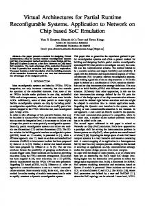
reconfigurable partition through the on-chip bus to control the computing process. 4.4.2. Architecture of Dynamic Reconfigurable Partition  Off-chip memory stores the input data and intermediate results for RUL prediction. Data exchange between the dynamic reconfigurable partition and off-chip memory is implemented in direct memory The internal structures of the reconfiguration units A and B are designed as shown in Figures 4  access (DMA) manner to improve data transmission efficiency. Decoupling IPs are used to avoid and 5. The internal architecture of the dynamic reconfigurable partition is a key factor to ensure the  disturbing the functions of static logic partition during dynamic reconfiguration. The configuration efficient task execution. The modular design is utilized to divide reconfiguration units A and B into  memory is used to store FPGATo  configuration files. several  computing  modules.  balance  the  resources  of  reconfigurable  units  and  leverage  the  parallel  computing  features  of  FPGA,  four  processing  elements  (PE)  of  kernel  functions  are  4.4.2. Architecture of Dynamic Reconfigurable Partition instantiated to synchronously calculate the Gaussian kernel.  In Figure 4, the reconfiguration unit A includes six main calculation modules, in which modules  The internal structures of the reconfiguration units A and B are designed as shown in 1–4  are 4parallel  PEs internal of  kernel  function,  module  5  is  a  matrix‐vector  multiplication  and  Figures and 5. The architecture of the dynamic reconfigurable partition is module,  a key factor module 6 is vector inner product module. The reconfiguration unit B shown in Figure 5 consists of  to ensure the efficient task execution. The modular design is utilized to divide reconfiguration five modules, in which module 1 is for matrix multiplication, module 2 is for improved Cholesky  units A and B into several computing modules. To balance the resources of reconfigurable units and decomposition, module 3 is for matrix inversion, module 4 is for matrix‐vector multiplication, and  leverage the parallel computing features of FPGA, four processing elements (PE) of kernel functions module 5 is for vector inner product.  are instantiated to synchronously calculate the Gaussian kernel. FPGA

Reconfigurable unit A Module 1

Data MUX output

RAM1

Kernel calculation 1

FIFO1

 Decoupling IP

Calculation Module 4 scheduling control Module 5 module Module 6

RAM4

Kernel calculation 4

FIFO4

RAM5

Matrix-vector multiplication

FIFO5

RAM6

Vector inner product

FIFO6

Data MUX

Data MUX control signals

  Figure 4. Internal structure of reconfiguration unit A. Figure 4. Internal structure of reconfiguration unit A. 

Energies 2016, 9, 572

10 of 19

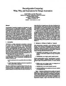
In Figure 4, the reconfiguration unit A includes six main calculation modules, in which modules 1–4 are parallel PEs of kernel function, module 5 is a matrix-vector multiplication module, and module 6 is vector inner product module. The reconfiguration unit B shown in Figure 5 consists of five modules, in which module 1 is for matrix multiplication, module 2 is for improved Cholesky decomposition, module 3 is for matrix inversion, module 4 is for matrix-vector multiplication, Energies 2016, 9, 572  10 of 18  and module 5 is for vector inner product. FPGA

Reconfigurable unit B Data MUX output Module 1

Module 2 Decoupling IP

Calculation scheduling Module 3 control module Module 4 Module 5

RAM1

RAM2

Matrix multiplication Improved Cholesky decomposition

FIFO1

FIFO2

RAM3

Matrix inversion

FIFO3

RAM4

Matrix-vector multiplication

FIFO4

RAM5

Vector inner product

FIFO5

Data MUX control signal

Data MUX

 

Figure 5. Internal structure of reconfiguration unit B.  Figure 5. Internal structure of reconfiguration unit B.

The  interface  between  the  reconfiguration  partition  and  the  static  logic  partition  must  be  The interface between the reconfiguration partition and the static logic partition must be consistent. consistent.  It  includes  on‐chip  bus  interface  and  the  control  interface  for  data  and  commands  It transmission. Calculation control module ensures that the computing tasks are executed in sequence  includes on-chip bus interface and the control interface for data and commands transmission. Calculation control module ensures that the computing tasks are executed in sequence with the with the scheduled timing. First‐in‐first‐out (FIFO) is for buffering the calculation results and RAM  scheduled timing. First-in-first-out (FIFO) is for buffering the calculation results and RAM is for is for buffering the input data and intermediate variables. The inputs and outputs of the FIFO and  buffering the input data and intermediate variables. The inputs and outputs of the FIFO and RAM are RAM are controlled by the Calculation control module related to specific computing task.  controlled by the Calculation control module related to specific computing task. 4.4.3. Design of Key Modules  4.4.3. Design of Key Modules The kernel function computing involves calculation of 2‐norm and exponential functions. The 2‐ The kernel function computing involves calculation of 2-norm and exponential functions. norm calculation has low computation efficiency since it cannot be executed with pipeline computing  The 2-norm calculation has low computation efficiency since it cannot be executed with pipeline while the exponential function is a transcendental function which cannot be directly implemented by  computing the exponential is a transcendental function cannot be directly multiplier while and  adder.  To  achieve function high  efficiency,  a  multi‐level  pipeline which calculation  method  of  implemented by multiplier and adder. To achieve high efficiency, a multi-level pipeline calculation piecewise  linear  approximation  is  proposed.  In  addition,  an  improved  Cholesky  decomposition  method  proposed  to  accommodate  the  large  of  computations  matrix  inversion  with  method ofis piecewise linear approximation is amount  proposed. In addition,in an improved Cholesky lower‐upper (LU) decomposition and the instability caused by the round‐off error from the Cholesky  decomposition method is proposed to accommodate the large amount of computations in matrix decomposition.  inversion with lower-upper (LU) decomposition and the instability caused by the round-off error from Multi‐level pipelined calculation method of piecewise linear approximation for the kernel function  the Cholesky decomposition. 2 2 For  Gaussian  kernel  function  K(x, xi )  exp( x  xi 2  )   where     is  the  hyper‐parameter  • Multi-level pipelined calculation method of piecewise linear approximation for the kernel function determined  before  training,  the  kernel  matrix  Φ   is  a  symmetric  positive  definite  matrix  whose  diagonal elements are all 1. Therefore, only the lower triangular elements, as shown below, need to  For Gaussian kernel function Kpx, xi q “ expp´||x ´ xi ||22 {γ2 q where γ is the hyper-parameter be calculated:  determined before training, the kernel matrix Φ is a symmetric positive definite matrix whose diagonal elements are all 1. Therefore, only the lower elements, as shown 1  triangular  below, need to be calculated: k ( x , x )  1 » fi 2 1  1     (20) lower  k ( x3 , x1 ) k ( x3 , x2 )  —Φkpx ffi 1  — ffi 2 , x1 q 1    — ffi   .. — ffi . k ( x , x )1 Φlower “ — kpx3 , x1kq( xn kpx (20) , x q ffi 3 2 , ) ( , ) x k x x  1 2 n n n 1  — ffi .. .. .. — ffi – fl . . . 1 (a) 2‐Norm Calculation  kpxn , x1 q kpxn , x2 q ¨ ¨ ¨ kpxn , xn´1 q 1 l , the 2‐norm for vector  x i   and  x j   is:  Assuming that the dimension of training samples is  xi  x j

2 2

 ( xi1  x j1 ) 2  ( xi 2  x j 2 ) 2    ( xil  x jl ) 2  

(21)

A multi‐level pipelined method is introduced to calculate the 2‐norm. Take the first column in 

Energies 2016, 9, 572

(a)

11 of 19

2-Norm Calculation Assuming that the dimension of training samples is l, the 2-norm for vector xi and x j is: ||xi ´ x j ||22 “ pxi1 ´ x j1 q2 ` pxi2 ´ x j2 q2 ` ¨ ¨ ¨ ` pxil ´ x jl q2

(21)

A multi-level Energies 2016, 9, 572 

pipelined method is introduced to calculate the 2-norm. Take the first column 11 of 18 in Equation (20) as an example, the computing elements are shown in Table 1. Table 1. Computing components for the 2‐norm computation.  Table 1. Computing components for the 2-norm computation. th 1st Step  2nd Step     l  Step 

2‐Norm  2 1 2   ||x2 ´ x1 ||22 2 ||x3 ´ x31 ||221 2

2-Norm x x

2 a1 1st( xStep 21  x11 )

2

x x

..  . ||xn ´xx1 ||x22 n

2 1 2

a1 “ px21 ´ x11 q22 a  (x  x ) a2 2“ px3131´ x1111q2 ..  . 22 an´1 a n 1“px ( xn1n1´ xx11 11 q)

Step 2 a n  (2xnd 22  x12 )

 ¨¨¨

a ( l 1)*（ n -1 ）+1  ( xl2thl Step x1l ) 2

¨¨¨ apl´1q˚pn´1q`1 “ px22l ´ x1l q2 a “ px ´ x q2 a x1lpx ) ´ x q2  n-1） 2  (x3l “ (l 1)* ¨¨¨ a（pl´1q˚pn´1q`2 an`1 “ px32 ´ x12 q2 3l 1l ..  ...  ...  . 2 a（ ““ px ´ x1l q2 aann`n´2 ( x npx  x´12 x) 212 q2  ¨ ¨ ¨ a(l 1)*  ( x pl´1q˚pn´1q`n`1 2 n2 n2  “ n-1） n-1 nl  x1l ) nl

a n 1n  ( x3222 x1212) 2

2

The  2‐norm  computing  process  is  executed  by  rows.  That  is,  x 2  x1 2   is  first  and  then  The2 2-norm computing process is executed by rows. That is, ||x2 ´ x1 ||22 is first and then 2 x||x 3 3 x so  so forth.  In  this  process,  a  fully  pipelined  accumulator  is is designed  with  ´1 x1, ||and  , and forth. In this process, a fully pipelined accumulator designed withan  anfully  fully pipelined adder and a FIFO as shown in Figure 6.  pipelined adder and a FIFO as shown in Figure 6.

Figure 6. The fully pipelined accumulator.  Figure 6. The fully pipelined accumulator.

Figure 7 shows the computing flowchart of the fully pipelined accumulator. In the first stage,  Figure 7 shows the computing flowchart of the fully pipelined accumulator. In the first stage, data a1, a2,...,an−1 and “0“ are input to the adder, and the outputs of the adder are stored in the FIFO.  data a1 , a2 , ..., an ´1 and “0“ are input to the adder, and the outputs of the adder are stored in the FIFO. In the 2ndnd  stage, data an, an+1,...,a2(n−1) and FIFO buffered data from the 1st stage are then input to the  In the 2 stage, data an , an+1 , ..., a2(n´1) and FIFO buffered data from the 1st stage are then input to adder. The outputs of the adder are again stored in the FIFO. This process is repeated at the lth pipeline th the adder. The outputs of the adder are again stored in the FIFO. This process is repeated at the l cycle. Similarly, the 2‐norm calculations in other columns can be implemented.  pipeline cycle. Similarly, the 2-norm calculations in other columns can be implemented. Stage 

Stage 1st 

1st 2nd 

2nd … 

...

Index  1  Index 2  1…  2n−1  ... 1  n´1 2  1 …  2 n−1  ... … 

n´1 . . .1  1 2  2…  . .n.−1  n´1

Input data 1  InputaData a2  a…  1 aa2n−1  ... an  an ´1 an+1  an …  an+1 a2*(n−1)  ... …  a2*(n ´1) a( l .1)*.（.n 1）+1  

FIFO Output 0  Output FIFO 0  …  0 0  0 ... a1  0 a2  a1 …  a2 an−1  ... …  an ´1 a1+an+…+  a ( l  2 )*（ n  1 ）+ 1  

... a21+ a n+1 +…+   a a + a + . . . + a（pnl ´ ( l  2 )*  12 ）q˚p  2 n´1q`1 n lth  a + a + . . . + a 2 n+1 …  pl ´2q˚pn´1q`2 lth an‐1+ a2*(n‐1)+…+ a. (.l . 1)*（ n  1 ）   an´1 + a2˚(n´1) + . . . + apl ´1q˚pn´1q Figure 7. The computing flowchart of pipelined accumulator.    apl ´a1(q˚p l 1)* （ 11 ）q` 2 1 nn´ apl ´1q˚p…  n´1q`2 a. l（ .* n.1）  al ˚pn´1q

Figure 7. The computing flowchart of pipelined accumulator.

(b) Exponential Function Calculation  Since exponential function cannot be implemented directly by adders and multipliers in FPGA,  a piecewise linear approximation method, which combines linear polynomial function and LUT, is  employed as an approximation [25]. In this method, the linear polynomial parameters are stored in  the LUT while the calculation of linear polynomial is implemented by an adder and a multiplier in FPGA.  The  principle  of  piecewise  linear  approximation  is  as  follows:  for  a  nonlinear  function  f ( x)  

Energies 2016, 9, 572

(b)

12 of 19

Exponential Function Calculation

Since exponential function cannot be implemented directly by adders and multipliers in FPGA, a piecewise linear approximation method, which combines linear polynomial function and LUT, is employed as an approximation [25]. In this method, the linear polynomial parameters are stored in the LUT while the calculation of linear polynomial is implemented by an adder and a multiplier in FPGA. The principle of piecewise linear approximation is as follows: for a nonlinear function f pxq defined in x P rL, Us, the interval is evenly divided into m subintervals [Li , Ui ] and m “ pU ´ Lq{pUi ´ Li q. For x P rLi , Ui s, f pxq is approximated as f pxq “ k i x ` bi , where k i and bi are linear polynomial parameters stored in the LUT. Note that m introduces trade-off between accuracy and hardware Energies 2016, 9, 572  12 of 18  occupation and should be selected properly. Figure 8 shows the data path of Gaussian kernel function calculation. In this figure, the upper Figure 8 shows the data path of Gaussian kernel function calculation. In this figure, the upper  part is for 2-norm calculation while the lower part is for exponential function calculation. In the lower part is for 2‐norm calculation while the lower part is for exponential function calculation. In the lower  part, bRAM and kRAM store parameters k and b for piecewise linear approximation, respectively. part, bRAM and kRAM store parameters k and b for piecewise linear approximation, respectively.  The corresponding values of k and b can be obtained by accessing the addresses for these The corresponding values of k and b can be obtained by accessing the addresses for these two  two RAMs. Then the kernel function can be calculated with subtractor 2 and multiplier 4. To get the RAMs. Then the kernel function can be calculated with subtractor 2 and multiplier 4. To get the right  right addresses of bRAM and kRAM, the output of the 2-norm calculation is mapped to the RAM addresses of bRAM and kRAM, the output of the 2‐norm calculation is mapped to the RAM address  address by multiplication, “floating-point to fixed-point” and rounding units. by multiplication, “floating‐point to fixed‐point” and rounding units. 

  Figure 8. The computing circuits for the Gaussian kernel function.  Figure 8. The computing circuits for the Gaussian kernel function.

Since the computing delay of multiplier 4 is one clock cycle larger than subtractor 2, FIFO4 is  Since the computing delay of multiplier 4 is one clock cycle larger than subtractor 2, FIFO4 is used to synchronize them by introducing a clock delay to access the bRAM. FIFO3 is used to store  used to synchronize them by introducing a clock delay to access the bRAM. FIFO3 is used to store the the output of 2‐norm calculation and its depth should be larger than the delay of multiplier 4, which  output of 2-norm calculation and its depth should be larger than the delay of multiplier 4, which is is 8 clock cycles in this design. The multiplier and adder are implemented with Xilinx floating‐point  8 clock cycles in this design. The multiplier and adder are implemented with Xilinx floating-point arithmetic IP core, and the data are in single‐precision floating point format.  arithmetic IP core, and the data are in single-precision floating point format.  Improved Cholesky decomposition for matrix inversion based on multiply subtraction  • Improved Cholesky decomposition for matrix inversion based on multiply subtraction To make computations affordable and deal with the instability caused by rounding error in of  matrix inversion computing process, an improved Cholesky decomposition [26] is introduced for the  To make computations affordable and deal with the instability caused by rounding error in of matrix inversion computing process, an improved Cholesky [26] is introduced for inversion  of  symmetric  positive  definite  Gaussian  kernel  decomposition matrix   .  The  improved  Cholesky  ř the inversion of symmetric positive definite  Gaussian kernel matrix . The improved Cholesky decomposition method decomposes matrix  ř   as follows:  decomposition method decomposes matrix as follows:T (22)   LDL   ÿ T “ LDL (22) where L is a lower triangular matrix whose diagonal elements are all 1, D is a diagonal matrix (its  diagonal elements are not 0). Matrices L and D can be obtained as:    r 1    2 d r   hrr   lrk d k  , k  1     r 1    lir   hir   lik d k lrk  / d r . k 1     

where  r  1,, n, i  r  1,, n   and  h  is the element of   . 

(23)

Energies 2016, 9, 572

13 of 19

where L is a lower triangular matrix whose diagonal elements are all 1, D is a diagonal matrix (its diagonal elements are not 0). Matrices L and D can be obtained as: $ ˆ ˙ rř ´1 ’ ’ 2 d ’ d “ h ´ l rr & r rk k , k “1 ˆ ˙ rř ´1 ’ ’ ’ lir “ hir ´ lik dk lrk {dr . %

(23)

k “1

ř where r “ 1, ¨ ¨ ¨ , n, i “ r ` 1, ¨ ¨ ¨ , n and h is the element of . ř Assuming P “ L´1 , we have ´1 “ PT D´1 P, where P is a lower triangular matrix with elements of: $ ’ & pii “ 1{lii “ 1 iř ´1 iř ´1 (24) lik pkj “ ´ lik pkj ’ % pij “ ´pii k“ j

k“ j

where i “ 1, 2, ¨ ¨ ¨ n, j “ 1, 2, ¨ ¨ ¨ i ´ 1. Energies 2016, 9, 572  13 of 18  The implementation of the improved Cholesky decomposition and matrix inversion is shown in ´ 1 Figure 8. The elements in diagonal matrix D is the reciprocal of corresponding elements in matrix D D and this only requires division. The computation of matrix P, i.e., the inverse matrix of L, is given by  and this only requires division. The computation of matrix P, i.e., the inverse matrix of L, is given by pii  1   and  p ij   is the negative value of the result from a multiply accumulator:  Equation (24), in which  Equation (24), in which pii “ 1 and pij is the negative value of the result from a multiply accumulator:

di

divider 1

FIFO1

-1

D pij

U

lik pkj

multiplier 1

FIFO2 subtracter 1

 

Figure 9. The data path for matrix inversion.  Figure 9. The data path for matrix inversion.

In Figure 9, the calculation of D−1 is achieved with divider 1 and the results are stored into FIFO1.  In Figure 9, the calculation of D´1 is achieved with divider 1 and the results are stored into FIFO1. Multiplier 1, subtractor 1 and FIFO2 are used to calculate the pij, in which FIFO2 buffers the results  Multiplier 1, subtractor 1 and FIFO2 are used to calculate the pij , in which FIFO2 buffers the results −1 from the subtractor 1, which is initialized as 0. The memory depth of FIFO1 and FIFO2 is n. With D   from the subtractor 1, which is initialized memory depth of FIFO1 and FIFO2 is n. With D´1 1 1 as T0. The 1 ř´ ř  =P D P and P,    can be calculated by  .  1 and P, can be calculated by ´1 “ PT D´1 P. 5. 5. Discussion System Performance Testing and Evaluation  Discussion System Performance Testing and Evaluation  

5.1. Hardware Platform  5.1. Hardware Platform The run‐time dynamic RC system must be implemented on reconfigurable devices for onboard  The run-time dynamic RC system must be implemented on reconfigurable devices for onboard and distributed applications. To verify the proposed run‐time dynamic RC system for RVM‐based  and distributed applications. To verify the proposed run-time dynamic RC system for RVM-based lithium‐ion  batteries  estimation,  the ML510 Xilinx development ML510  development  board  is experiments, used.  In  the  lithium-ion batteries RULRUL  estimation, the Xilinx board is used. In the experiments,  accuracy,  computational  efficiency,  and consumption hardware  resource  consumption  RVM for  the  accuracy, computational efficiency, and hardware resource for the reconfigurable reconfigurable RVM based RUL prediction system are analyzed and discussed.  based RUL prediction system are analyzed and discussed. The main specifications for ML510 development board are as follows:  The main specifications for ML510 development board are as follows:  FPGA: Virtex XC5VFX130T;  ‚ FPGA: Virtex XC5VFX130T;  DDR2 SDRAM: 512MB, 72‐bit and 2 chips;  ‚ DDR2 512 MB, 72-bit and 2 chips;  SDRAM: CompactFlash (CF): 512MB.  A  run‐time  RC  system  is  constructed  as  shown  in  Figure  10,  in  which  the  embedded  ‚ CompactFlash (CF):RVM  512 MB. processor  PowerPC440  has a  working frequency  of 400  MHz,  the  on‐chip  PLB  bus  has  a  working  A run-time RC RVM system is constructed as shown in Figure 10, in which the embedded frequency set to 100 MHz, the configuration port is the ICAP interface embedded in the XC5VFX130T,  processor PowerPC440 has a working frequency of 400 MHz, the on-chip PLB bus has a working and the floating‐point arithmetic computing is implemented with the single‐precision floating‐point  IP  core  based  on  IEEE754  standard  [27]  provided  by  Xilinx  ISE  13.2  (San  Jose,  CA,  USA).  For  comparison purposes, a PC platform with a 2.53 GHz Core 2 Duo CPU, and 2 G DDR2 memory is  used to execute the same algorithm.  5.2. Lithium‐ion Battery Data Set 

Energies 2016, 9, 572

14 of 19

frequency set to 100 MHz, the configuration port is the ICAP interface embedded in the XC5VFX130T, and the floating-point arithmetic computing is implemented with the single-precision floating-point IP core based on IEEE754 standard [27] provided by Xilinx ISE 13.2 (San Jose, CA, USA). For comparison purposes, a PC platform with a 2.53 GHz Core 2 Duo CPU, and 2 G DDR2 memory is used to execute the same algorithm. 5.2. Lithium-Ion Battery Data Set Two lithium-ion battery data sets are used to verify the proposed framework. One is from the data repository of the NASA Ames Prognostics Center of Excellence (PCoE) and the other one is from the CALCE at the University of Maryland. The first data set was sampled from a battery prognostics test bed at NASA comprising commercially available Li-ion 18650 rechargeable batteries [28]. The lithium-ion batteries were run through three different operational profiles (charge, discharge, and impedance) at room temperature. Charging was carried out in a constant current mode at 1.5 A until the battery voltage reached 4.2 V and then continued in a constant voltage mode until the charge current dropped to 20 mA. Discharge was carried out at a constant current level of 2 A until the battery voltage fell to 2.7 V, for battery B5. Repeated charge and discharge cycles resulted in accelerated aging of the batteries. The experiments were stopped when the batteries reached the end-of-life criterion, which was a 30% Energies 2016, 9, 572  14 of 18  fade in rated capacity.

LAN PCI Slots DDR2 Virtex XC5VFX130T

SDRAM

CF Controller CompactFlash Development Board

Monitor

Power supply

Emulator

Figure 10. The run-time RC RVM system with ML510 development board. Figure 10. The run‐time RC RVM system with ML510 development board. 

InIn the CALCE data set, the cycling of battery CS2‐33 was implemented with the Arbin BT2000  the CALCE data set, the cycling of battery CS2-33 was implemented with the Arbin BT2000 battery  testing  system(made  by  Arbin  Instruments,  College TX, Station,  TX,  USA)  under  room  battery testing system (made by Arbin Instruments, College Station, USA) under room temperature. temperature.  The  1.1  Ah  capacity  of  batteries  adopted with in  the  the  The 1.1 Ah rated capacity ofrated  batteries are adopted in theare  experiment theexperiment  dischargingwith  rate at discharging rate at 0.5 C [15,29].  0.5 C [15,29].

5.3. Prediction Precision of RUL Estimation  In this Section, the battery data sets are used to verify the performance of the run‐time dynamic  RC system for RVM, and the results are compared with those from the PC platform. The quantitative  prediction  results  for  B5  and  CS2‐33  batteries  are  summarized  in  Table  2.  The  prediction  starting  points are selected at the 80th cycle for B5 battery and 278th cycle for the CS2‐33 battery, respectively.  The failure thresholds for the two batteries are set to 1.38 Ah (about 30% fade) and 0.88 Ah (about  20% fade). In this table, the performances are compared by the predicted RUL (RULp) values (given 

Energies 2016, 9, 572

15 of 19

5.3. Prediction Precision of RUL Estimation In this Section, the battery data sets are used to verify the performance of the run-time dynamic RC system for RVM, and the results are compared with those from the PC platform. The quantitative prediction results for B5 and CS2-33 batteries are summarized in Table 2. The prediction starting points are selected at the 80th cycle for B5 battery and 278th cycle for the CS2-33 battery, respectively. The failure thresholds for the two batteries are set to 1.38 Ah (about 30% fade) and 0.88 Ah (about 20% fade). In this table, the performances are compared by the predicted RUL (RULp) values (given by the mean of the predicted RUL distribution), the Absolute Error (AE) (given by the difference between the actual RUL (RULa) and RULp), the predicted precision ratio of two platforms (η AE ) (given by the ratio of absolute difference of AE to RULa), and 95% confidence intervals (CI). Table 2. RUL prediction comparison between FPGA and Matlab. Index B5 CS2-33

Platform FPGA PC FPGA PC

RULa 48 240

RULp (mean)

95% CI

AE

45 49 231 225

[34, 49] [41, 54] [222, 248] [208, 238]

3 1 9 15

η AE 4.2% 2.5%

From Table 2, it is clear that the results from the two platforms have comparable accuracy. The prediction precisions on the RC platform are 4.2% and 2.5% different from that on the PC platform for the two batteries. This is because the RC platform uses single-precision computing while the PC platform adopts double-precision computing, but these minor differences are acceptable for industrial applications. Note that the predicted confidence intervals from the two platforms are very close to each other. The experimental results show that RUL prediction with dynamic reconfigurable RVM on the FPGA platform is comparable to the prediction on the PC platform. 5.4. Analysis of Computing Efficiency To quantify the improvement on computational efficiency of the proposed method, the computing processes of lithium-ion battery RUL prediction in Section 4.3 is analyzed. The speed-up ratio is defined as: T (25) ηt “ PC´RV M TRC´RV M where TRC-RVM is the executing time with RC platform and TPC-RVM is with PC platform. It is clear that ηt > 1 indicates that the RC-based RVM algorithm has higher computational efficiency than the PC platform. The larger the ηt , the higher the increase of the efficiency. Table 3. Efficiency comparison between FPGA and PC. Index B5

CS2-33

Platform

TT (ms)

PT (ms)

N.R

O.R (ms)

OT (ms)

FPGA PC Speed-up ηt FPGA PC Speed-up ηt

96.70 614.02 6.35 524.25 6287.30 11.99

7.32 11.81 1.61 69.27 185.62 2.68

2 0 0 2 0 0

16.99 0.00 0.00 16.99 0.00 0.00

138.00 625.83 4.54 627.50 6472.92 10.31

TT; Training time; PT: Predicting time; N.R: No. of reconfigurations; O.R: Overhead per reconfiguration; OT: Overall time.

The comparison is summarized in Table 3, which shows that RC based RVM in FPGA has higher efficiency than the PC platform in terms of training, prediction, and overall. For prediction part with low computational complexity, the speed-up ratios for the battery B5 (small prediction steps) and

Energies 2016, 9, 572

16 of 19

the battery CS2-33 (relatively large prediction steps) are 1.61 and 2.68, respectively. For training part with high computational complexity, the speed-up ratios for the battery B5 and the battery CS2-33 are 6.35 and 11.99, respectively. As for the overall efficiency, the speed-up ratios for the two batteries are 4.54 and 10.31, respectively. This demonstrates that the proposed RC-based RVM in FPGA platform has great potentials in improvement of computational efficiency, especially for complex tasks. The FPGA power is about 4.94 W by Xilinx Power Estimator and the power of the CPU is about 25 W from its datasheet, so the FPGA consumes 0.68 J and 3.10 J energy, which are 22.97ˆ and 52.17ˆ less than CPU, for B5 and CS2-33 RUL prediction, respectively. This further demonstrates that FPGA is more suitable for embedded and power aware application. 5.5. Analysis of Hardware Resource Consumptions To verify the adaptability and applicability of the proposed method, the hardware resources, including the utilization of static and dynamic partition throughout the FPGA, are analyzed. The analysis also shows the improvement of resource utilization of the dynamic RC against the static reconfiguration. The required hardware resources of RC RVM approach and the available FPGA resources are shown in Table 4. The utilization ratio of DSP48E and BRAM is larger than that of LUTS (the logic resources) in our proposed method. This suits to the characteristics of the computing with FPGA IP core in which more DSP48E and BRAM resources are consumed. Note that more than 50.00% of the BRAM and DSP48E resources in FPGA are reserved, which demonstrates that the proposed method has great potentials to support more complex computation tasks with limited computing resources. And in another aspect, a smaller FPGA device, such as XC5VFX70T, can be used to accommodate the whole design. This better fits the requirements of the compact embedded BMS systems. Table 4. FPGA resource utility. Categories

PowerPC

LUTs

BRAM

DSP48E

Static partition Dynamic partition Total utilized resources Total FPGA resources Ratio of utilization

1 0 1 2 50.00%

4826 14,144 18,970 81,920 23.16%

48 40 88 298 29.53%

0 120 120 320 37.50%

The improvement of the resources utilization by the dynamic RC algorithm can be further illustrated by comparing the resources occupation of the dynamic RC and static reconfiguration. The resource consumptions of dynamic area are obtained by Xilinx’s Plan Ahead design tool and the results are compared in Table 5. In Table 5, the resources consumption in the static reconfigurable algorithm is the sum of the reconfigurable units A and B, without considering the increased connectivity resources consumption. For dynamic RC, the resources consumption is those in the dynamic partition. Table 5 shows the dynamic resources saving includes 9408LUTs (39.95%), 15 BRAM (27.27%), and 62 DSP48E (34.07%). This result demonstrates that the proposed method has higher FPGA resource utilization and is more suitable for computing resources constrained applications. Table 5. The increase of hardware utility. Items

LUTs

BRAM

DSP48E

Reconfigurable unit A Reconfigurable unit B Sum of two units Dynamic Dynamic partition Resources saving Resources saving percentage

9440 14,112 23,552 14,144 9408 39.95%

21 34 55 40 15 27.27%

90 92 182 120 62 34.07%

Static

Energies 2016, 9, 572

17 of 19

The difference of DSP48E for two reconfigurable units in static reconfiguration is 2, which accounts for 2.17% of the maximum required DSP48E resources (92). This shows that the two reconfigurable units achieve the consumption balance of DSP48E. This further proves the effectiveness of the proposed method using multi-objective optimization for reconfigurable tasks partitioning in which the balance of DSP48E resources between different partitions is the main constraint. The static reconfigurable implementation can be realized with logics combining reconfigurable unit A and reconfigurable unit B in DPR version. Then the training and forecasting process will consume the same time with DPR version, but it avoids two reconfiguration overheads (2 ˆ 16.99 ms). From Table 3, the reconfiguration overheads are about 24.6% and 5.4% in the whole consumed time of the B5 and CS2-33 batteries’ prognosis respectively. By avoiding these overheads, the static reconfigurable implementation can get 1.33ˆ and 1.06ˆ speedup in B5 and CS2-33 batteries respectively compared to the corresponding dynamic reconfigurable implementation. Thus static reconfigurable implementation can get the computational performance a little bit improved, but at the cost of more hardware consumption as shown in Table 5 (39.95% more LUTs, 27.27% more BRAM, 34.07% more DSP48E). Regarding our motivation to get a more compact BMS, we think dynamic reconfigurable system is a better choice. 6. Conclusions In this work, a novel run-time dynamic RC-based RVM prognostic algorithm and its implementation on a reconfigurable FPGA platform are developed for RUL estimation. The experiment results demonstrate that the embedded computing platform can significantly improve the computing efficiency and flexibility. The contributions of the research work include a balance of resources utilization and computing efficiency is achieved by multi-objective optimization method to implement computing tasks partitioning; the multi-level pipelined computing and parallel computing are developed for kernel function calculation to further improve the computational efficiency; the improved Cholesky decomposition for matrix inversion is introduced to reduce the computing resource consumption and decreases the computational delay; and thorough analysis and comparison of different embedded system configurations in terms of accuracy, resource utilization, and computation efficiency. Experimental results on two examples of lithium-ion battery RUL estimation show that the FPGA based run-time dynamic RC improves the hardware resources utilization and is more than four times faster than a PC-based approach without sacrificing performance. This work provides a novel solution for the implementation of prognostic prediction based on machine learning algorithm in embedded computing systems. In future, more algorithms, such as SOC estimation, prognosis in operation condition varying applications, etc., will be implemented in the proposed system. Acknowledgments: This work was partially supported by the National Natural Science Foundation of China (Grant No. 61571160 and 61301205), Fundamental Research Funds for the Central Universities (Grant No. HIT.NSRIF.201615), Guangxi Key Laboratory of Automatic Detecting Technology and Instruments (YQ15201), and China Scholarship Council. Author Contributions: Shaojun Wang, Datong Liu and Yu Peng conceived and designed the experiments; Shaojun Wang and Jianbao Zhou performed the experiments and analyzed the data; Shaojun Wang, Datong Liu and Bin Zhang wrote the paper. Conflicts of Interest: The authors declare no conflict of interest.

References 1. 2.

Liu, D.; Wang, H.; Peng, Y.; Xie, W.; Liao, H. Satellite lithium-ion battery remaining cycle life prediction with novel indirect health indicator extraction. Energies 2013, 6, 3654–3668. [CrossRef] Chaoui, H.; Golbon, N.; Hmouz, I.; Souissi, R.; Tahar, S. Lyapunov-Based Adaptive State of Charge and State of Health Estimation for Lithium-Ion Batteries. IEEE Trans. Ind. Electron. 2015, 62, 1610–1618. [CrossRef]

Energies 2016, 9, 572

3. 4. 5.

6. 7. 8.

9. 10. 11. 12. 13. 14. 15. 16.

17. 18. 19.

20.

21.

22. 23.

24.

18 of 19

Xiao, R.; Shen, J.; Li, X.; Yan, W.; Pan, E.; Chen, Z. Comparisons of Modeling and State of Charge Estimation for Lithium-Ion Battery Based on Fractional Order and Integral Order Methods. Energies 2016, 9. [CrossRef] Zhang, C.; Wang, L.; Li, X.; Chen, W.; George, G.Y.; Jiang, J. Robust and Adaptive Estimation of State of Charge for Lithium-Ion Batteries. IEEE Trans. Ind. Electron. 2015, 62, 4948–4957. [CrossRef] Gholizadeh, M.; Salmasi, F.R. Estimation of state of charge, unknown nonlinearities, and state of health of a lithium-ion battery based on a comprehensive unobservable model. IEEE Trans. Ind. Electron. 2014, 61, 1335–1344. [CrossRef] Zhang, B.; Tang, L.; Jonathan, D.; Michael, R.; Kai, G. Autonomous Vehicle Battery State-of-Charge Prognostics Enhanced Mission Planning. Int. J. Progn. Heal. Manag. 2014, 5, 1–11. Shahriari, M.; Farrokhi, M. Online State-of-Health Estimation of VRLA Batteries Using State of Charge. IEEE Trans. Ind. Electron. 2013, 60, 191–202. [CrossRef] Muñoz-Condes, P.; Gomez-Parra, M.; Sancho, C.; Andrés, M.A.G.S.; González-Fernández, F.J.; Carpio, J.; Guirado, R. On Condition Maintenance Based on the Impedance Measurement for Traction Batteries: Development and Industrial Implementation. IEEE Trans. Ind. Electron. 2013, 60, 2750–2759. [CrossRef] Long, B.; Xian, W.; Jiang, L.; Liu, Z. An improved autoregressive model by particle swarm optimization for prognostics of lithium-ion batteries. Microelectron. Reliab. 2013, 53, 821–831. [CrossRef] Liu, J.; Wilson, W.; Farid, G. A multi-step predictor with a variable input pattern for system state forecasting. Mech. Syst. Signal. Process. 2009, 23, 1586–1599. [CrossRef] Andre, D.; Appel, C.; Soczka-Guth, T.; Sauer, D.U. Advanced mathematical methods of SOC and SOH estimation for lithium-ion batteries. J. Power Sources 2013, 224, 20–27. [CrossRef] Orchard, M.O.; Hevia-Koch, P.; Zhang, B. Risk Measures for Particle-Filtering-Based State-of-Charge Prognosis in Lithium-Ion Batteries. IEEE Trans. Ind. Electron. 2013, 60, 5260–5269. [CrossRef] Zhang, B.; Chris, S.; Carl, B.; Romano, P.; Marcos, E.O.; George, V. A Probabilistic Fault Detection Approach: Application to Bearing Fault Detection. IEEE Trans. Ind. Electron. 2011, 58, 2011–2018. [CrossRef] Tipping, M.E. Sparse Bayesian Learning and the Relevance Vector Machine. J. Mach. Learn. Res. 2001, 1, 211–244. Wang, D.; Miao, Q.; Michael, P. Prognostics of lithium-ion batteries based on relevance vectors and a conditional three-parameter capacity degradation model. J. Power Sources 2013, 239, 253–264. [CrossRef] García, G.J.; Jara, C.A.; Pomares, J.; Alabdo, A.; Poggi, L.M.; Torres, F. A Survey on FPGA-Based Sensor Systems: Towards Intelligent and Reconfigurable Low-Power Sensors for Computer Vision, Control and Signal Processing. Sensors 2014, 14, 6247–6278. [CrossRef] [PubMed] Kang, M.; Kim, J.; Kim, J.M. An FPGA-Based Multicore System for Real-Time Bearing Fault Diagnosis Using Ultrasampling Rate AE Signals. IEEE Trans. Ind. Electron. 2015, 62, 2319–2329. [CrossRef] Souza, A.C.D.; Fernandes, M.A.C. Parallel Fixed Point Implementation of a Radial Basis Function Network in an FPGA. Sensors 2014, 14, 18223–18243. [CrossRef] [PubMed] Romero-Troncoso, R.J.; Saucedo-Gallaga, R.; Cabal-Yepez, E.; Garcia-Perez, A.; Osornio-Rios, R.A.; Alvarez-Salas, R.; Miranda-Vidales, H.; Huber, N. FPGA-based online detection of multiple combined faults in induction motors through information entropy and fuzzy inference. IEEE Trans. Ind. Electron. 2011, 58, 5263–5270. [CrossRef] Fons, F.; Fons, M.; Cantó, E.; López, M. Real-time embedded systems powered by FPGA dynamic partial self-reconfiguration: A case study oriented to biometric recognition application. J. Real-Time Image Process. 2013, 8, 229–251. [CrossRef] Mentens, N.; Vandorpe, J.; Vliegen, J.; Braeken, A.; Silva, B.; Touhafi, A.; Kern, A.; Knappmann, S.; Rettkowski, J.; Kadi, M.S.A.; et al. DynamIA: Dynamic Hardware Reconfiguration in Industrial Applications. Appl. Reconfig. Comput. 2015, 9040, 513–518. Wang, C.; Liu, Y.L.; Jiang, P.L.; Zhang, Q.Z.; Tao, F.; Zhang, L. Multiple Faults Detection with SoC Dynamic Reconfiguration System Based on FPGA. Advance Mater. Res. 2013, 694, 2642–2645. [CrossRef] He, Y.; Wang, S.; Peng, Y.; Pang, Y.; Ma, N.; Pang, J. High performance relevance vector machine on HMPSoC. In Proceedings of the 2014 International Conference on Field-Programmable Technol, Shanghai, China, 10–12 December 2014; pp. 334–337. Wang, S. Research on Reconfigurable Computing for Time Series Forecasting. Ph.D. Thesis, Harbin Institue of Technology, Harbin, China, June 2012.

Energies 2016, 9, 572

25. 26.

27.

28. 29.

19 of 19

Omondi, A.R.; Rajapakse, J.C. FPGA Implementations of Neural Networks; Springer: Dordrecht, The Netherlands, 2006; pp. 21–34. Yang, D.; Peterson, G.D.; Li, H.; Sun, J. An FPGA Implementation for Solving Least Square Problem. In Proceedings of the 17th IEEE Symposium on Field-Programmable Custom Computing Machines, Napa, CA, USA, 5–7 April 2009; pp. 303–306. 754-2008-IEEE Standard for Floating-Point Arithmetic. Available online: http://ieeexplore.ieee.org/ xpl/articleDetails.jsp?arnumber=5976968&queryText=IEEE%20754&refinements=4294965216 (accessed on 12 July 2016). Battery Data Set, NASA Ames Prognostics Data Repository. Available online: http://ti.arc.nasa.gov/project/ prognostic-data-repository (accessed on 20 February 2016). Xing, Y.; Ma, E.W.M.; Tsui, K.; Pecht, M. An ensemble model for predicting the remaining useful performance of lithium-ion batteries. Microelectron. Reliab. 2013, 53, 811–820. [CrossRef] © 2016 by the authors; licensee MDPI, Basel, Switzerland. This article is an open access article distributed under the terms and conditions of the Creative Commons Attribution (CC-BY) license (http://creativecommons.org/licenses/by/4.0/).