A self-adaptive multi-engine solver for quantified Boolean formulas
Recommend Documents
the placement of alternating quantifiers, QSAT is complete for each class in the ..... The first six solvers above are pure search-based engines, i.e., they are an ...
Feb 12, 2012 - AI] 12 Feb 2012. Message passing for quantified Boolean formulas. Pan Zhang1, Abolfazl Ramezanpour1, Lenka Zdeborová2, and Riccardo.
Email: [email protected]. Supported by a NSF. Graduate Research Fellowship. quantified Boolean formulas (QBF). QBF is a general- ization of the satisfiability ...
D. Mundici. Satisfiability in many-valued sentential logic is NP-complete. Theoretical Com- puter Science, 52(1-2):145â153, 1987. 27. G. Priest. Logic of paradox ...
Many reasoning task and combinatorial problems exhibit symmetries. ... Solving Quantified Boolean Formulas (QBF) has become an attractive and important ...
Via Sommarive 18, 38055 Povo, Trento, Italy [email protected]. Abstract. A certificate of satisfiability for a quantified boolean formula is a compact representation of.
by harnessing inductive reasoning techniques to learn engine-selection policies. Our second result is the improvement of our multi-engine solver with the ...
on Presburger Arithmetics, i.e., Boolean combinations of linear constraints. From a theoretical perspective, we clar- ify the problem of the treatment of universal ...
Center for Applied Mathematics ... call that SAT is known to be NP-complete, and QBF is known ..... by the solver (in particular, overflow occurred). 3 Theoretical ...
note n mutually disjoint sets of variables that are quantified by. Q1 ...Qn, respectively. ..... [9] G. Gopalakrishnan, Y. Yang, and H. Sivaraj. QB or not QB: An effi-.
Bibliography. 157. [33] James P. Delgrande, Torsten Schaub, Hans Tompits, and Stefan Woltran. ... [40] Rainer Feldmann, Burkhard Monien, and Stefan Schamberger. A distributed al- ... [41] Ian P. Gent, Peter Nightingale, and Kostas Stergiou.
Here we focus on approaches that are mainly based on mathematical logic ...... Algorithm 2 the parameter T is the trail of literals assumed by previous ...... of times (5 in our implementation) we give up on SAT solving for this descent ...... The ha
Apr 12, 2011 - the case of Horn formulas in order to find small representations of knowledge bases [HK95]. .... A B-formula/circuit Ï and a natural number k.
gence (www.aaai.org). All rights reserved. 1999a; Pan, Sattler, & Vardi ... tial two-player games with complete information. For in- stance, â{a}â{b}â{c}â{d}Φ ...
siderably more subtlety required in encodings in QBF than in SAT. Second, in an area such as QCSP where algorithmic techniques are not yet highly developed, ...
Abstract. We present a Probably Approximate Correct (PAC) learning paradigm for boolean formulas, which we call PAC meditation, where the class of formulas.
Consider a QBF of the form (1). A literal Ð occurring in ¨ is: â existential if Ð belongs to the prefix of (1), and is universal otherwise. â unit in (1) if Ð is existential, ...
uses a propagation-based constraint solver. It is based on ... Some of these solvers provide special-purpose boolean solvers while others have been .... a constant (0 or 1), or an expression of the form ite(x, F, G), meaning âif x then .... ing a f
To deal with the problem, we propose a hard disk backed Breadth. First Search .... fix Q on the resultant clause set, the resulting formula is the core QBF formula.
which is seen as a useful complement to the standard unit clause resolution step ... prefix p is a supergraph (Z, E) of the Gaifman graph of Ï along with and ...
Feb 6, 2017 - [1] George Boole. An Investigation of the Laws of thought. Walton, London, 1854. [2] F. M. Brown. Boolean reasoning. The logic of Boolean ...
We start from a reasonable C++ STL (standard template library) version of the kernel .... variable, but employ heuristics and machine learning to decide which ...
Formulas Represented by Embedded Cycles. Guillermo De Ita Luna, ... By other way, many combinatorial problems ask about embeddings of graphs into other ...
Uwe Egly, Thomas Eiter, Volker Klotz, Hans Tompits, and Stefan Woltran. Technische ..... ated QBFs are translated into definitional normal form (Eder. 1992 ...
A self-adaptive multi-engine solver for quantified Boolean formulas
Abstract. In this paper we study the problem of engineering a robust solver for quantified. Boolean formulas (QBFs), i.e., a tool that can efficiently solve formulas ...
A self-adaptive multi-engine solver for quantified Boolean formulas Luca Pulina DIST, Universit`a di Genova, Viale Causa, 13 – 16145 Genova, Italy
Abstract In this paper we study the problem of engineering a robust solver for quantified Boolean formulas (QBFs), i.e., a tool that can efficiently solve formulas across different problem domains without the need for domain-specific tuning. The paper presents two main empirical results along this line of research. Our first result is the development of a multi-engine solver, i.e., a tool that selects among its reasoning engines the one which is more likely to yield optimal results. In particular, we show that syntactic QBF features can be correlated to the performances of existing QBF engines across a variety of domains. We also show how a multi-engine solver can be obtained by carefully picking state-of-the-art QBF solvers as basic engines, and by harnessing inductive reasoning techniques to learn engine-selection policies. Our second result is the improvement of our multi-engine solver with the capability of updating the learned policies when they fail to give good predictions. In this way the solver becomes also self-adaptive, i.e., able to adjust its internal models when the usage scenario changes substantially. The rewarding results obtained in our experiments show that our solver AQME – Adaptive QBF Multi-Engine – can be more robust and efficient than state-of-the-art single-engine solvers, even when it is confronted with previously uncharted formulas and competitors.
1
Introduction
The problem of evaluating quantified Boolean formulas (QBFs) is one of the cornerstones of Complexity Theory. In its most general form, it is the prototypical PSPACEcomplete problem, also known as QSAT [1]. Introducing limitations on the number and the placement of alternating quantifiers, QSAT is complete for each class in the polynomial hierarchy (see, e.g., [2]). Therefore, QBFs can be seen as a low-level language in which high-level descriptions of several hard combinatorial problems can be encoded to find a solution by means of a QBF solver. The quantified constraint satisfaction
1
problem is one relevant example of such classes (see, e.g., [3]), and it has been shown that QBFs can provide compact propositional encodings in many automated reasoning tasks, including formal property verification of circuits (see, e.g., [4, 5, 6]), symbolic planning (see, e.g. [7, 8, 9, 10]) and reasoning about knowledge (see, e.g., [11, 12]). To make the QBF-based approach effective, solvers ought to be robust, i.e., able to perform well across different problem domains without the need for domain-specific tuning. However, as the results of the yearly QBF solvers competitions [13] clearly show, QBF solvers are rather brittle. The cause of this phenomenon can be traced back to the fact that all state-of-the-art QBF solvers implement some kind of heuristic algorithm. Indeed, every such algorithm will occasionally find problem instances that are exceptionally hard to solve, while the very same instances may easily be tackled by resorting to another algorithm, or by using a different heuristic. To the best of our current knowledge, brittleness across problem domains is not typical of QSAT, and it seems to be unavoidable for every combinatorial problem that is at least NP-hard (see, e.g., [14]). In the case of QSAT, if PSPACE-hard problems are indeed a tougher arena than NP-hard problems, then the state of affairs for QBF solvers can only be worse than, e.g., propositional satisfiability (SAT). In this paper we study the problem of engineering a robust QBF solver, i.e., a tool that can efficiently solve formulas across different problem domains without the need for domain-specific tuning. An important prerequisite of our study is the availability of performance data about QBF solvers, both in line with the current state of the art, and also quantitatively relevant in order to enable meaningful experimental setups. In the following, we consider the two most recent competitions of QBF solvers (QBFEVAL’06 and QBFEVAL’07) [13] as a source of formulas and solvers. Our first research result, obtained using QBFEVAL’06 data, is the development of a multi-engine solver, i.e., a tool that can choose among its engines the one which is more likely to yield optimal results with respect to the current state of the art. To this end, we show that a set of inexpensive syntactic QBF features are discriminative enough as to indicate the best kind of solver to run on each formula. While in principle a large set of features coming from diverse representations of the input formula could be used (see, e.g., [15, 16]), we considered relatively basic parameters such as the number of variables, the number of clauses, and the number of quantifier alternations. Indeed, our results show that it pays off to favor simple representations – and thus speed of computation – over complex ones. Harnessing inductive reasoning techniques, and carefully selecting a few QBFEVAL’06 competitors as basic engines, we obtained a multi-engine solver that is able to learn its engine-selection policies. We accomplish this by analyzing the performances of various inductive models, both symbolic, i.e., decision trees [17] and rules [18], and functional (sub-symbolic), i.e., multinomial logistic regression [19] and nearest-neighbor [20]. In the context of QBFEVAL’06 data, we show that our multi-engine solver is more robust than each single engine, and that it is also stable with respect to various perturbations applied to the dataset on which it is engineered. We also show that such a multi-engine solver can be competitive on a previously “unseen” dataset such as, in our case, the one of QBFEVAL’07. While the above results are encouraging, the performances of the plain multi-engine solver on the QBFEVAL’07 dataset suggest that further improvements can be sought. Our second result is a self-adaptive multi-engine solver, i.e., a multi-engine solver that 2
can update its learned policies when the usage scenario changes substantially. We accomplish this by studying the empirical run-time distributions of the solvers participating to QBFEVAL events, to find out that most solvers either manage to evaluate the formulas in a few seconds, or they fail even when allowing them several minutes of CPU time. From this observation, we design an adaptation schema that we call retraining, and we apply it to the engine selection-policies whenever they fail to give good predictions. Retraining works according to three key parameters: the time granted to the predicted engine, the order in which alternative engines are tried once retraining is triggered, and the time granted to each such trial. If the retraining procedure finds an alternative engine which solves a given formula in place of the initially predicted one, then our solver can update its internal models accordingly, and leverage the new model thereafter. Clearly, the exact values of the above parameters may depend on the formulas to be solved, on the run-time distributions of the basic engines, and on the inductive models used to learn the selection policy. At least on the QBFEVAL’07 dataset, we show that it is possible to obtain settings that can fit a wide range of QBFs, solvers, and all the inductive models that we have tried. The solver resulting from the above process is called AQME, for Adaptive QBF Multi-Engine, and we implemented it as a proof-of-concept system to validate our approach. AQME can be freely downloaded for research and evaluation purposes from http://www.mind-lab.it/aqme, and it is based on eight state-of-the-art solvers as of QBFEVAL’06, namely 2 CLS Q, QUAFFLE, QUANTOR, Q U BE, S K IZZO, SSOLVE and Y Q UAFFLE. AQME participated hors-concours in QBFEVAL’07 and, as such, it was not ranked among the regular QBFEVAL’07 competitors. However, the three versions of AQME would have ranked in the top three positions if AQME were running as a regular competitor. The rewarding results obtained during QBFEVAL’07 and in our experiments, show that the methodology described above and implemented in AQME can effectively enable it to self-adapt and improve its performances, even when confronted with previously uncharted formulas and/or competitors. The paper is structured as follows. In Section 2 we discuss the scientific literature to which our work relates the most. In Section 3 we review the syntax of QBFs and the features that we use to represent them. In Section 4 we outline the essentials of the QBFEVAL’06/07 events, with particular emphasis on the contestants, the formulas used, and their relationship with the QBFLIB collection. In Section 5 we discuss the design of AQME P LAIN, the plain multi-engine version of AQME. In Section 6 we show the experimental evaluation of AQME P LAIN, including the analyses regarding its stability, and the performances of AQME P LAIN on the QBFEVAL’07 dataset. In Section 7 we present the design issues behind the self-adaptive component of AQME, while in Section 8 we consider the tuning and experimental evaluation of AQME on the QBFEVAL’07 dataset. We conclude the paper in Section 9 with some final remarks. We have also added two appendices that contain, respectively, details about QBF features (Appendix A), and all the tables that are too large to fit nicely within the text of the paper (Appendix B).
3
2
Related work
Our approach can be related to the literature on algorithm portfolios [14, 21] for the solution of hard combinatorial problems. Our direct source of inspiration has been the work on the SATZILLA solver portfolio for SAT [22, 15]. More recent contributions that are also strictly related to our work include [16, 23], wherein improvements to the original SATZILLA framework are presented. Both [14, 21] do not consider machine learning techniques in order to learn the engine selection policy, whilst the results of [22, 15, 16, 23] are limited to SAT. Since QSAT is a generalization of SAT, our work considers problem classes in PSPACE that extend beyond NP, and provides results that are typical of such classes. Moreover, while SATZILLA performs quite well on so called “real-world” encodings (see, e.g., [23]), its tuning and experimental evaluation is performed mostly in the context of “artificial” benchmark problems, such as, e.g., random k-SAT [24]. In our case, we only consider QBFs coming from encodings – see Section 4 – which, because of their peculiarities, can be much harder to characterize and tame using inductive techniques. This paper builds partially on [25], wherein the plain multi-engine approach herewith discussed was introduced. In [26] an independent contribution along the same lines of [25] is made. Noticeably, in [26] the authors use a QBF solver as a grey-box to study the problem of dynamically adapting its heuristics using machine learning techniques whereas, by contrast, our approach always uses solvers as black-boxes and focuses on how to yield optimal results by combining their strengths. The work herewith presented provides more detailed explanations, analyses and further experimental results in the parts common to [25] and [26]. Moreover, the retraining algorithms, their application to build adaptive multi-engines, and the related tuning and experimentation have been studied neither in [26, 25] nor – to the best of our knowledge – in any of the related literature. Other related literature includes contributions on exploiting case-based reasoning to obtain algorithm portfolios for CSP solvers (see, e.g., [27]), whilst less recent work in the CSP context that also relates to ours includes [28], wherein algorithm selection by performance prediction is applied to the context of branch and bound algorithms. Finally, as it was pointed out by a reviewer, the work in [29] bears some resemblance with our adaptation mechanism, with the important difference that updated models are not retained in the framework of [29] as we do in ours.
3
Quantified Boolean Formulas: syntax and features
Consider a set P of propositional letters. A variable is an element of P. A literal is a variable or the negation of a variable. In the following, for any literal l, |l| is the variable occurring in l, and l is ¬l if l is a variable, and is |l| otherwise. A literal is positive if |l| = l and negative otherwise. A clause C is an n-ary (n ≥ 0) disjunction of literals such that, for any two distinct disjuncts l, l0 in C, it is not the case that |l| = |l0 |. A propositional formula is a k-ary (k ≥ 0) conjunction of clauses. A QBF is an expression of the form Q1 Z1 ...Qk Zk Φ 4
k≥0
(1)
where, for each 1 ≤ i ≤ k, Qi is a quantifier, either existential Qi = ∃ or universal Qi = ∀, such that Qi 6= Qi+1 , and the set of variables Zi = zi,1 , . . . zi,mi is a quantified set. The expression Qi Zi stands for Qi zi,1 . . . Qi zi,mi , and Φ is a propositional formula in the variables Z1 , . . . , Zk . The expression Q1 Z1 . . . Qk Zk is the prefix and Φ is the matrix of (1). A literal l is existential if |l| ∈ Zi for some 1 ≤ i ≤ k and ∃Zi belongs to the prefix of (1), and it is universal otherwise. In the prefix, k − 1 is the number of alternations, and k − i + 1 is the level of all the variables contained in the set Zi (1 ≤ i ≤ k); the level of a literal l is the same as |l|. Similarly to variables, if Qi = ∃ then the quantified set Zi is existential, and universal otherwise. For example, the expression: ∀y1 ∃x1 ∀y2 ∃x2 x3 {{y1 , y2 , x2 }, {y1 , ¬y2 , ¬x2 , ¬x3 }, {y1 , ¬x2 , x3 }, {¬y1 , x1 , x3 }, {¬y1 , y2 , x2 }, {¬y1 , y2 , ¬x2 }, {¬y1 , ¬x1 , ¬y2 , ¬x3 }, {¬x2 , ¬x3 }}
(2)
is a QBF with 8 clauses, where the variables y1 , y2 are universal, and x1 , x2 , x3 are existential; (2) contains four quantified sets, three alternations, and the levels of y1 , x1 , y2 , and x2 , x3 are 4,3,2 and 1, respectively. Notice that if Qk = ∀, then (1) becomes Q1 Z1 . . . ∃k−1 Zk−1 Φ0 , where Φ0 is obtained from Φ by deleting all the occurrences of the variables in Zk . Also, if there is at least one clause in Φ such that all of its literals are universal, then (1) is trivially false. In the following, without loss of generality, we assume that Qk = ∃, and that all the clauses have one existential literal at least, as in the example (2). In order to perform inductive inference on QBFs, we transform them into vectors of numeric values, where each value represents a specific feature. In particular, we consider several basic features, such as, e.g., the number of clauses, the number of variables, and the number of quantifier alternations. Among these features we also tried to consider parameters that should be somehow related to the algorithmic properties of different engines such as, e.g., the proportions in the number of universal and existential variables/literals, and the number of positive/negative occurrences of the variables. We also consider combined features, i.e., ratios and products of the basic features. These include, e.g., the product of the positive and negative occurrences of a variable, and several ratios including, e.g., the clause-to-variables ratio, the universal-to-existential ratio, and the positive-to-negative occurrences ratio. A complete listing of all the features that we have considered is given in Appendix A. The choice of the above features is dictated by several factors, including previous related work (see, e.g. [22]), inexpensiveness, and specific considerations about the nature of QBFs. Notice that some features, such as the number of clauses and the number of variables, yield a very abstract representation of QBFs, i.e., specific values of such features may correspond to several – possibly diverse – QBFs. On the other hand, distributions such as, e.g., the number of literals per clause, or the number of variable occurrences, give a more detailed representation of the underlying QBF, at the expense of an increased complexity. For each distribution we consider only its mean and its standard deviation from the mean, measuring the center and the spread of the distribution, respectively. Overall, for each QBF we compute 141 features, which is a fairly large number compared to 5
previous related work – SATZILLA [22] computes “only” 83 features. However, the median CPU time spent to compute all the 141 features, e.g., on the QBFEVAL’06 formulas, is 0.04s (min. 0.00s, max. 2.04s), so it is not too expensive to keep all of them.
4
QBFEVAL: solvers and formulas
All the experiments described from Section 5 to Section 8 are obtained using the solvers and the formulas participating in the QBFEVAL’06 and QBFEVAL’07 competitions of QBF solvers, i.e., the first and the second competition of QBF solvers, respectively, and the last two events in a series dating back to 2003 [13]. All the formulas used in QBFEVAL’06/07 are also part of the QBFLIB [30] collection, which is also the largest available repository of QBFs in the QDIMACS [31] format. Our decision of focusing on QBFEVAL’06 and QBFEVAL’07 rests on the fact that they are the largest public collections of recent performance data about QBF solvers. However, we also show that the variety of formulas used in QBFEVAL’06/07 is indeed representative of the variety that can be found in QBFLIB. To assess how much QBFEVAL’06/07 datasets are representative of the space of available formulas, hereafter in this section we also make use of QBFLIB formulas which never entered either QBFEVAL’06 or QBFEVAL’07. We will also briefly describe QBFEVAL’06/07 events inasmuch it is required to support the analyses presented in this paper. More details about the events can be found in [13], while a synopsis of the datasets extracted from such events is provided in Table 5 (Appendix B). The solvers out of which AQME is built are a subset of the contestants participating in QBFEVAL’06, where 16 versions of 11 solvers were run, namely OPEN QBF, QBFL, QUAFFLE, Q U BE, SSOLVE, Y Q UAFFLE , 2 CLS Q, PRE Q UANTOR , QUANTOR , S K IZZO and SQBF – see [13] for references. The first six solvers are pure search-based engines, i.e., they are an extension to QSAT of the DLL algorithm for SAT [32], while the other ones are based on a variety of techniques such as Q-resolution [33], skolemization (see, e.g., [34]), variable expansion (see, e.g., [35]), or a combination thereof, possibly including also search like, e.g., 2 CLS Q1 and S K IZZO. Formulas used in QBFEVAL’06 were submitted to the competition and picked from QBFLIB. The latter are a subset of the ones used in QBFEVAL’05 [36], where for each QBF, we compute a coefficient H [37] which ranges from 0 (easy, all the competitors solved the formula) to 1 (hard, none of the competitors solved the formula). QBFEVAL’05 formulas used in QBFEVAL’06 have 0.3 ≤ H < 1. In this paper we consider fixed structure formulas (FSFs for short) used in QBFEVAL’06. Intuitively, FSFs are resulting from encodings and/or artificial generators where a setting of the problem parameters yields a unique instance (see [36]). The reason why we are focusing on such formulas is that they are the most interesting ones for applications of QBF solvers when facing automated reasoning tasks in various domains. QBFEVAL’06 ran in two tracks: the short track, where the solvers were limited to 600 CPU seconds, and the marathon track, where 1 2 CLS Qis indeed a multi-stage solver: a preprocessor is run in the first stage, and the solver QUANTOR is run in the second stage; if the second stage is not successful within a short time limit, a third stage based on a search-based decision procedure is accomplished.
6
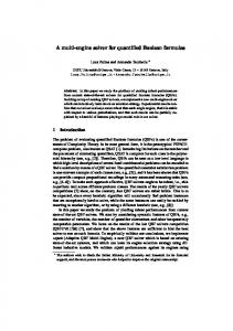
we alloted a time limit of 6000 CPU seconds. The memory was limited to 900MB in both tracks. Considering the results of the marathon track, out of 427 FSFs, 371 were solved (87% of the initial selection), 234 (55%) were declared satisfiable and 137 (32%) were declared unsatisfiable. The top-five solvers were: 2 CLS Q, PRE Q UANTOR, SQBF , S K IZZO -0.9- ABS and QUANTOR . Q U BE5.0, running hors-concours, was the best search-based solver, and it would have ranked fifth if running as a regular competitor. When speaking of the “QBFEVAL’06 dataset”, as in Table 5 (top), we refer to a subset of 318 formulas obtained from those that were actually solved, discarding those that were easily solved by most of the competitors. In QBFEVAL’07, 17 version of 11 solvers – including an early version of AQME running hors-concours – participated in the contest.2 Three solvers, besides AQME, feature a multi-engine approach or similar adaptation mechanisms, namely A DAP TIVE 2 CLS Q 3 , Q SS and Q Z ILLA (see [26]). As for the remaining single-engine solvers, three of them are search-based, namely AIGQBF, NC Q U BE, and Y Q UAFFLE, while the remaining ones are mainly based on other techniques: EBDDRES is based on Qresolution, SQUOLEM is purely skolemization-based, while QUANTOR and S K IZZO combine several techniques, including search as well. The formulas used in QBFEVAL’07 were submitted to the competition and recycled from QBFEVAL’06 according to the same rule described for QBFEVAL’06. Only FSFs formulas have been considered in QBFEVAL’07, and a single track limited to 600 CPU seconds and 900 MB of main memory was run. Considering the results of such track, out of 1136 FSFs, 873 were solved (77% of the initial selection), 353 (40%) were declared satisfiable, and 520 (60%) were declared unsatisfiable. The top-three solvers were S K IZZO (two versions), and QUANTOR, but the three versions of AQME would have ranked in the top-three positions if AQME were running as a regular competitor. When speaking of the “QBFEVAL’07 dataset” as in Table 5 (bottom), we refer to a set of 890 formulas which includes all the formulas used in QBFEVAL’07 that have not been recycled from QBFEVAL’06. As we said before, our decision of focusing on QBFEVAL’06/07 solvers and formulas has stringent practical motivations, since these are the only datasets for which a considerable number – about 20 solvers and one thousand formulas – of recent performance data are available. On the other hand, one may ask whether focusing on such datasets is oblivious of some important category of QBFs, i.e., one without which the scope of our analyses would be too limited. To show that this is indeed not the case, we computed the features described in Appendix A for all the FSFs currently available in QBFLIB, which amounts to consider 3383 formulas. In Figure 1 we report the results of the comparison between the variety of formulas in QBFLIB with respect to the variety of formulas in the QBFEVAL’06/07 datasets. The plot in Figure 1 (topleft) is obtained by considering each formula as a point in the multidimensional feature space. The coordinates of each formula thus correspond to the value computed for each of the 141 features considered. Since it is impossible to visualize such a space, we consider its two-dimensional projection obtained by means of a principal compo2 One solver, P QBF [38], entered the non-prenex non-cnf solver contest, but we do not consider it here since all of our work is done for prenex-CNF QBFs, i.e., formulas as defined in Section 3. 3 Technically speaking, A DAPTIVE 2 CLS Q is a multi-stage solver (like 2 CLS Q) featuring an adaptive heuristic in the search component.
7
Cluster ID Formulas QBFEVAL06 QBFEVAL07
1 1738 17% 44%
2 108 6% 39%
3 501 14% 2%
4 342 11% 23%
5 694 3% –
Figure 1: Coverage of the QBFLIB collection by QBFEVAL’06/07 formulas (top-left), clustering of QBFLIB (top-right), and percentage of QBFEVAL’06/07 formulas in each cluster (bottom). nents analysis (PCA) and considering only the first two principal components (PC).4 The x-axis and the y-axis in the plot are the first and the second PCs, respectively. Each point is a formula, either a circle (QBFLIB), a square (QBFEVAL’06), or a diamond (QBFEVAL’07). A quick glance at the plot of Figure 1 (top-left) reveals that the variety of QBFLIB is covered – albeit not completely – by the QBFEVAL’06/07 datasets. To get a quantitative picture of the phenomenon, in Figure 1 (top-right), we present a clustering of QBFLIB, and in Figure 1 (bottom), the relationship between the clusters and the QBFEVAL’06/07 datasets. The clustering is obtained using partition around medoids (PAM), a classical divisive clustering algorithm [40]. We estimate the number of clusters using the silhouette coefficient of clustering quality [40], where the silhouette value is computed for each element of a cluster, ranging from -1 (bad) to 1 (good). We consider optimal the clustering such that the average silhouette is maximized, and we choose the number of clusters accordingly. In Figure 1 (top-right), five clusters yielded the maximum average silhouette value of 0.7. In Figure 1 (bottom) we can see that all the clusters – with the exception of cluster #5 in the QBFEVAL’07 datasets – are partially represented in the QBFEVAL’06/07 dataset, and that the biggest cluster (#1) is covered for more than 50%. In particular: • Cluster #1 has many more representatives in the QBFEVAL’07 dataset since all of the formulas in the “Herbstritt” suite (see [41]) have been submitted for QBF4 Details about PCA and its use for visualizing multidimensional datasets are beyond the scope of this paper: see, e.g., Chap. 7 of [39] for an introduction to PCA and further references.
8
EVAL’07. • Cluster #2 is also more heavily represented in QBFEVAL’07 because of the whole “Palacios” and part of the “Mangassarian” suites. • Cluster #3 is comprised mainly of problems that have been progressively discarded from QBFEVAL datasets because of their relative simplicity; it also includes formulas that participated hors-concours in QBFEVAL’07; in view of such data, the relative small coverage of this cluster by QBFEVAL’06/07 datasets does not seem to be critical for their usefulness. • Cluster #4 is comprised mainly by part of the “Mangassarian” suite, the “Biere/Counter” problems5 , some “Ansotegui” problems (never run in an evaluation), several easy formulas (considering 2005 state-of-the-art solvers), and the “Mneimneh-Sakallah” suite (see [4]) which, on the other hand, is comprised of relatively hard formulas (considering 2007 state-of-the-art solvers). • Cluster #5 is scarcely covered; it is comprised mainly of “Gent-Rowley” encodings (see [42]) used in QBFEVAL’04, and “Ansotegui” encodings (see [10]) used in QBFEVAL’05; notice that most of these formulas have been discarded from QBFEVAL’06/07 because of their relative simplicity. Summing up, we can say that QBFEVAL’06/07 datasets sample – albeit not proportionally – all the classes that can be “naturally” identified using the features which we use to describe QBFs. Moreover, the under-represented classes tend to correspond either to excessively easy or hard formulas, which are not very interesting for our purposes.
5
AQME P LAIN :
Designing a multi-engine solver
In this section we review the design of AQME P LAIN, i.e., we do not consider the adaptive component which we introduce in Section 7. Here we focus on the basic design issues by looking at the choice of features, the choice of inductive models, and the choice of basic engines. All the experiments that we present hereafter ran on a farm of 10 identical rack-mount PCs, equipped with 3.2GHz PIV processors, 1GB of RAM and running Ubuntu/GNU Linux (distribution Edgy 6.10). The first design issue when developing AQME P LAIN is whether the features mentioned in Section 3 are sufficient to determine the best engine to run on each formula. We would like our features to be at least as descriptive as to discriminate between search-based solvers and the remaining ones, that we call “hybrid” in the following. Considering the QBFEVAL’06 dataset only, we remove 194 formulas that were solved both by search and hybrid solvers, to end up with 124 formulas that are solved either by search solvers or hybrid ones, but not by both. We apply PAM to classify the formulas, and, as before, we estimate the number of clusters using the silhouette coefficient. In our experiments, eleven clusters yielded the maximum average silhouette value of 5 “Biere/Counter” problems are artificially generated toy model checking problems for counter circuits and they are not part of the “Biere” suite in QBFEVAL’06/07 which, on the other hand, includes realistic model checking problems.
9
Cluster ID Formulas Search Hybrid 2 CLS Q OPEN QBF PRE Q UANTOR QUANTOR Q U BE3.0 Q U BE4.0 Q U BE5.0 SQBF S K IZZO -0.9- ABS S K IZZO -0.9- STD SSOLVE SSOLVE - UT SSOLVE + UT Y Q UAFFLE
Table 1: Classification of formulas according to their features and correspondence with solvers. 0.9.6 Finally, we compare the clusters with the percentage of formulas solved by search and hybrid solvers respectively. If the initial choice of features was a good one, then we expect to find a clear correlation between cluster membership and the likelihood of being solved by a particular kind of solver. In Table 1 we present the results of the above analysis. In the table, each column corresponds to a cluster (Cluster ID) where we detail the number of formulas in the cluster (Formulas), the percentage of such formulas that were solved by search solvers (Search), and by hybrid solvers (Hybrid), respectively. In this table we do not report data related to QUAFFLE and QBFL because these solvers are not able to solve any of the formulas considered. The results in Table 1 show that, with the only exception of clusters #2 and #3, our choice of features enables us to automatically partition QBFs into classes such that we can predict whether the best solver in each class is searchbased or not. This is an indication that the features we consider are good candidates to hint the best engine to run on each formula. As a side effect, we can also see that our distinction between search and hybrid solvers does make sense, at least on the QBFEVAL’06 dataset. Indeed, search solvers perform badly on the clusters #6 – #11 dominated by hybrid solvers, while on the other clusters, either search solvers dominate, or there is always at least one search solver that performs better than any hybrid one. The second design issue concerns the inductive models to implement in AQME P LAIN. An inductive model is comprised of a classifier, i.e., a function that maps an unlabeled instance (a QBF) to a label (a solver), and an inducer, i.e., an algorithm that builds the classifier. In the following, we call training set the dataset on which inducers are trained, and test set the dataset on which classifiers are tested. While there is an overwhelming number of inductive models in the literature (see, e.g., [39]), we 6 Notice that the starting dataset is a subset of the one used in Figure 1; technically, while both classifications are optimal – in the average silhouette sense – the one we are considering here is at a finer level of granularity than the one considered in Figure 1.
10
can somewhat limit the choice considering that AQME P LAIN has to deal with numerical attributes (QBF features) and multiple class labels (engines). Moreover, we would like to avoid formulating specific hypotheses about the features, and thus we prefer inducers that are not based on hypotheses of normality or (in)dependence among the features. Finally, we also prefer inducers that do not require complex ad-hoc parameter tuning. Considering all the above, we chose to implement four inductive models in AQME P LAIN , namely: Decision trees (C4.5) A classifier arranged in a tree structure, wherein each inner node contains a test on some attributes, and each leaf node contains a label; we use C4.5 [17] to induce decision trees. Decision rules (R IPPER) A classifier providing a set of “if-then-elsif” constructs, wherein the “if” part contains a test on some attributes and the “then” part contains a label; we use RIPPER [18] to induce decision rules. Logistic regression (MLR) A classifier providing a linear estimation, i.e., a hyperplane, of the hypersurfaces that separate the class labels in the feature space; we use the multinomial logistic regression (MLR) inducer described in [19]. 1-nearest-neighbor (1NN) A classifier yielding the label of the training instance which is closer to the given test instance, whereby closeness is evaluated using some proximity measure, e.g. Euclidean distance; we use the method described in [20] to store the training instances for fast lookup. The above methods are fairly robust, efficient, they are not subject to stringent hypotheses7 on the training data, and they do not need complex parameter tuning. They are also “orthogonal”, as they use algorithms based on radically different approaches. The last, but not in order of importance, design issue that we faced in AQME P LAIN is the choice of the state-of-the-art solvers that should be used as basic engines. Focusing on the QBFEVAL’06 competitors, a quick inspection in the results of Table 1 reveals that at least one search and one hybrid solver should be selected. The question remains whether only two competitors, all sixteen of them, or some other intermediate selection would be best. In the following, we consider all the above cases by comparing three versions of AQME P LAIN: AQME P LAIN 2, obtained using only two engines, namely 2 CLS Q and Q U BE5.0; AQME P LAIN 16, obtained using all sixteen QBFEVAL’06 marathon track contestants; AQME P LAIN 8, an informed selection among QBFEVAL’06 contestants, wherein we include five search solvers, namely Q U BE3.0, Q U BE5.0, SSOLVE - UT, QUAFFLE, and Y Q UAFFLE, and three hybrid ones, namely 2 CLS Q, QUANTOR, and S K IZZO -0.9- STD. In the following, we will refer to S K IZZO 0.9- STD as S K IZZO, and to SSOLVE - UT as SSOLVE. In Table 6 (Appendix B) we summarize the results of the comparison among the above versions of AQME P LAIN. The table contains the performance estimates on the QBFEVAL’06 dataset of AQME P LAIN 2, AQME P LAIN 16, and AQME P LAIN 8. In the 7 MLR is guaranteed to yield optimal discriminants – in the least squares sense – only when the dataset is partitioned into classes characterized by a multivariate normal distribution. If this is not the case, MLR can still provide us with a reasonable, albeit suboptimal, classification.
11
case of AQME P LAIN 2 the full dataset is a proper subset of the QBFEVAL’06 dataset, because we did not consider from the onset those formulas that could not be solved by either 2 CLS Q or Q U BE5.0. The data reported in Table 6 are obtained using a tentimes ten-fold stratified cross-validation (see [43]), whereby the dataset is divided into ten subsets, or folds, such that each subset is a stratified sample, i.e., it contains exactly the same proportions of class labels that are present in the original dataset. Once the folds are computed, nine out of ten are used for training an inducer, and the remaining one is used to test the classifier. The process is repeated ten times, each time using a different fold for testing, and thus yielding ten different samples of the measures of merit. For each inducer we consider as separate measures of merit (i) the number of formulas solved, and (ii) the cumulative CPU time of AQME P LAIN – including the default time limit value (600s) for the formulas that were not solved. While the usual way of comparing different inductive algorithms is to compare the ratio of correctly predicted formulas versus the total number of formulas in the test set (see, e.g., [39]), such definition would be misleading in our case since it assumes that all the wrong predictions have the same – unitary – cost. Indeed, in AQME P LAIN a wrong prediction has a cost which depends also on the solver predicted in place of the best one. For the sake of reference, Table 6 also reports about the best single-engine on the specific fold, i.e., the AQME P LAIN engine that is able to solve most problems (usually different among different folds), and the state of the art (SOTA) solver, i.e., the oracle that always fares the best time among AQME P LAIN engines. A preliminary consideration about the data shown in Table 6 concerns the fact that we do not report the time spent to train the inducer, to compute the features and to classify the instances, since it is always negligible with respect to the time spent to evaluate QBFs, except for AQME P LAIN 16 using MLR. In this case, we do not report any result, because the implementation of the inducer – based on the WEKA library [39] – could not complete the training phase on a single fold within 2400s of CPU time and 900MB of main memory on our hardware platform. Bearing the above in mind, a glance at Table 6 reveals that AQME P LAIN is better than the best single-engine on each fold in all the combinations of inductive models and basic engines. Since the best single-engine is not always the same, this means that AQME P LAIN can perform better than an ideal engine whose performances always correspond to the best single-engine solver on each fold. When it comes to the comparison among AQME P LAIN 2, AQME P LAIN 16, and AQME P LAIN 8, in Table 6 we can observe the following: • AQME P LAIN 2 is comparable to AQME P LAIN 8 and better than AQME P LAIN 16 in terms of accuracy in the number of problems solved. This is mostly due to the fact that discriminating among only two classes makes for a simpler classifier than discriminating among K > 2 classes. All other things being equal, our results confirm that the inducers can yield better classifiers when using a selection of only two engines. However AQME P LAIN 2 performances are generally worse than AQME P LAIN 8 in terms of speed, since the limited selection of engines constraints AQME P LAIN 2 to a suboptimal choice in many problem instances. • AQME P LAIN 16, on the other hand, is less accurate than AQME P LAIN 8 both in terms of number of problems solved and solution speed. This is mostly due to the fact that discriminating among sixteen engines makes for a noisier problem than 12
discriminating among eight – or between two. The noise mostly comes under the form of aliasing, i.e., instances that look like one another of which, say, one is easy and can be solved by almost all the engines, while the others are relatively hard and can be solved only by a few, possibly different, engines. Noise, and the relatively high number of classes among which the classifier must discriminate, limit the performance of the inductive models. This case is particularly evident in AQME P LAIN 16 when using R IPPER, but it is also true of all the other models which we were able to train and test. • AQME P LAIN 8 overall performances in terms of speed come within a factor of 4 with respect to the SOTA oracle in the worst case (R IPPER); C4.5 and MLR performances come within a factor of 3, and 1NN is only a factor of 1.5 slower than the SOTA oracle. To the above we must add that the oracle corresponding to AQME P LAIN 2 cannot solve as many problems as AQME P LAIN 16 and AQME P LAIN 8 oracles, simply because the selection of Q U BE5.0 and 2 CLS Q cannot solve as many problems as the other two selections can. Moreover, the performance problems observed about AQME P LAIN 16 using MLR limit its applicability, particularly when considering the methods proposed in Section 7. Summing up, AQME P LAIN 8 offers the best compromise between training time and accuracy, both in terms of number of problems solved and in terms of solution speed. The key point is that AQME P LAIN 8 engines are able to solve as many problems as AQME P LAIN 16 engines, and, at the same time, the restricted selection of engines keeps the aliasing noise to a tolerable level in AQME P LAIN 8. Notice that any further change in the composition of the engine pool, i.e., using less than eight solvers and/or picking different ones, results in suboptimal performances, at least according to our experiments on the QBFEVAL’06 datasets. In the following, we will refer to AQME P LAIN 8 simply as AQME P LAIN .
6
Experimental evaluation of AQME P LAIN
Since any classifier learned in AQME P LAIN will always be dependent on the training data – as in any approach based on inductive inference (see, e.g., [39]) – the real question is how strong is the dependence of AQME P LAIN from the dataset on which it is engineered. In this section we present two sets of experiments in order to quantify such dependence. In Section 6.1, we study the performances of AQME P LAIN under various perturbations of the QBFEVAL’06 dataset used for training and testing. In Section 6.2, we present some results on the QBFEVAL’07 dataset obtained by running AQME P LAIN against both its engines and the QBFEVAL’07 competitors.
6.1
(In)dependence of AQME P LAIN from the QBFEVAL’06 dataset
The set of experiments that we present in the following is meant to answer questions about the stability of AQME P LAIN, i.e., how much its performances change when the composition of the training/test sets is altered. In particular we consider
13
1. non-deterministic changes which alter the size of the sets, 2. deterministic changes which bias the training set in favor of easy problems, and 3. deterministic changes which bias the training set in favor of a given engine. All the experiments above are carried out using the QBFEVAL’06 dataset, and the platform outlined in Section 5. The engines are limited to 600s of CPU time, and 900MB of main memory. Our first experiment is aimed at understanding the effect of random changes in the size of the dataset used for training/testing. We compute several pairs of training/test sets by removing instances uniformly at random without repetition from the QBFEVAL’06 dataset. The removed instances are used to build test sets, while the remaining instances are used for training. By increasing the percentage of removed instances, we can increase the level of departure with respect to the original dataset, and thus we can assess the stability of our results with respect to an increasing perturbation. We remove 10% to 50% of the original instances, in increments of 10%, and we randomly generate 50 training/test sets for each percentage of removed instances. Table 7 (Appendix B) shows the results of our experiments. Considering the result therewith presented, we can conclude that the performances of AQME P LAIN are substantially stable and fairly independent of the relative composition of the training vs. the test sets. Notice that, considering the best case scenarios – except when training on 50% of the original dataset – at least one version of AQME P LAIN is able to solve all the formulas in the test set. Moreover, considering the number of formulas solved, AQME P LAIN features a ratio between best and worst case scenario that is closer to 1 than all its engines. This indicates that AQME P LAIN is more robust than its components for all but substantial departures from the QBFEVAL’06 dataset. Our second experiment is aimed at understanding how much AQME P LAIN is sensitive to perturbations that diminish the maximum amount of CPU time granted to the solvers. For this experiment, we considered four datasets extracted from QBFEVAL’06 by setting the time limit to 10, 5, 1 and 0.5 seconds, and then considering all the formulas that were solved by at least one competitor within each given time limit. We used the time-capped datasets as training sets, and the remaining instances as test sets. Notice that the size of the sets increases as the time limit decreases, so this experiment explores the possibility of training AQME P LAIN with a small number of easy-to-solve formulas, and then deploying it on a large number of hard-to-solve ones. Table 8 (Appendix B) shows the results of the above experiment. From the data therewith presented, we can conclude that even when training on relatively easy formulas, e.g., those that can be solved within 0.5 seconds by at least one competitor, the four AQME P LAIN versions perform substantially better than every other engine. This result confirms that AQME P LAIN models are relatively immune to changes in the training set that have an impact on the time resources alloted to the solvers. Our third experiment aims to establish how much AQME P LAIN is sensitive to a training set that is biased in favor of a given solver. For each engine, we consider all the formulas that it can evaluate within the allotted resources as the training set, and the remaining formulas as the test set. Table 9 (Appendix B) shows the results of the above experiment. 14
Considering the results of Table 9, we can see that a biased training set poses a serious challenge to AQME P LAIN, but, with the exception of the training set biased on QUANTOR , at least one of its versions is always the best solver in each group. According to the specific bias, a different version of AQME P LAIN, if any, is best. In particular, AQME P LAIN -1NN is the best solver when the bias is in favor of Q U BE3.0, Q U BE5.0 and Y Q UAFFLE; AQME P LAIN -C4.5, AQME P LAIN -R IPPER and AQME P LAIN -MLR are the best solvers when the bias is in favor of 2 CLS Q, SSOLVE, and QUAFFLE, respectively. Notice that when the bias is in favor of 2 CLS Q, Q U BE5.0, S K IZZO, and SSOLVE, then the solvers Q U BE5.0, and S K IZZO are very close to the performances of AQME P LAIN. These results can be explained if we consider that removing a specific solver may substantially alter the proportion of formulas in the training/test sets that are more likely to be solved by search rather than hybrid solvers. For instance, since Q U BE5.0 is the best search solver, the test set corresponding to the training set biased on Q U BE5.0 will be comprised almost completely by formulas that are more likely to be solved by hybrid solvers, which explains the good performances of S K IZZO with respect to AQME P LAIN in this case.
6.2
Testing AQME P LAIN on the QBFEVAL’07 dataset
In the second round of experiments, we train AQME P LAIN on the whole QBFEVAL’06 dataset, and we run on it the QBFEVAL’07 dataset. Remember from Section 4 that the QBFEVAL’07 dataset does not include any of the formulas in the QBFEVAL’06 dataset, so this is a typical deployment scenario, wherein the classifiers are used to predict the best solver on previously “unseen” QBFs. Again, all such experiments are carried out using the platform outlined in Section 5, where the engines are limited to 600s of CPU time, and 900MB of main memory. In Table 2 we show the results of the above experiments. The table is split horizontally in two parts, corresponding to two different scenarios (column “Scenario”). The former – reported on top of Table 2 – is about AQME P LAIN competing against its engines, and the latter – reported on the bottom of Table 2 – is about AQME P LAIN competing against the QBFEVAL’07 engines. In each part, the column “Solver” reports the name of a solver (either single- or multi-engine), and there are three groups of columns “Total”, “Sat”, and “Unsat”, corresponding to the overall performances, performances on formulas found to be satisfiable, and performances on formulas found to be unsatisfiable, respectively. In each group, the column “#” relates to the number of problems solved, and the column “Time” relates to the cumulative CPU time consumed to solve them – excluding formulas on which a solver exhausted the available resources. The table is sorted in descending order, according to the total number of formulas solved, and, in case of a tie, in ascending order according to the cumulative time to solve them. Looking at Table 2 (top), and considering that in this scenario 254 formulas out of 890 were not solved by any engine within the allotted resources, we can see that AQME P LAIN only partially confirms the results obtained on the QBFEVAL’06 dataset. In particular, the accuracy of MLR is higher than 1NN and substantially higher than C4.5 and R IPPER. The best solver on this dataset is now a single-engine solver, namely Q U BE5.0 with 495 formulas solved. MLR and 1NN, rank “only” second and third best, respectively, while C4.5 ranks below three of its engines, namely Q U BE5.0, 15
Scenario
AQME P LAIN vs. its engines
AQME P LAIN vs. QBFEVAL’07 engines
Solver Q U BE5.0 AQME P LAIN -MLR AQME P LAIN -1NN Q U BE3.0 S K IZZO AQME P LAIN -C4.5 2 CLS Q AQME P LAIN -R IPPER SSOLVE QUANTOR Y Q UAFFLE QUAFFLE AQME P LAIN -MLR NC Q U BE 1.0 NC Q U BE 1.1 S K IZZO QCK AQME P LAIN -1NN S K IZZO STD AQME P LAIN -C4.5 AQME P LAIN -R IPPER A DAPTIVE 2 CLS Q QUANTOR 2.15 Y Q UAFFLE SQUOLEM EBDDRES
Table 2: AQME P LAIN deployed on the QBFEVAL’07 dataset: AQME P LAIN vs. its engines (top), and AQME P LAIN vs. QBFEVAL’07 contestants (bottom). Q U BE3.0, and S K IZZO. Finally R IPPER ranks below all the other versions of AQME P LAIN and also below another of its engines (2 CLS Q). Overall, we can observe two phenomenons that call for an explanation. The first, is that AQME P LAIN is not the best solver any more. The explanation of this fact can be found considering the results of Section 6.1 about the effects of a training set biased in favor of a given solver. Indeed, the QBFEVAL’06 dataset that we are now using as training set is biased in favor of hybrid solvers: among the top five single-engine solvers on the QBFEVAL’06 dataset there is only one search-based solver, namely Q U BE5.0, and it ranks only fifth-best. On the other hand, the top five single-engines solver on the QBFEVAL’07 dataset are mostly search based: Q U BE5.0 (best), Q U BE3.0 (second best), and SSOLVE (fifthbest). Therefore, the QBFEVAL’07 dataset is clearly biased in favor of search-based solvers. As we have shown in Section 6.1, even a slight bias in favor of some kind of solver can alter the performances of AQME P LAIN. In the case of Table 2 scenarios, the data tell us that the difference in bias between QBFEVAL’06 and QBFEVAL’07 is indeed pretty heavy, which explains the overall results of AQME P LAIN. The second fact, is that different AQME P LAIN version “react” to the unseen dataset in different ways. Comparing the results of Table 2 (top) with those of Table 6 (bottom), we can see that MLR is more robust than 1NN, even if cross-validation would suggest otherwise. Moreover, while R IPPER remains the worse among AQME P LAIN models, C4.5 is now much worse than MLR. While we do not have a definite explanation of this phenomenon, we conjecture that both 1NN and C4.5, tend to overfit the training model. In the presence of an heavy difference between training and test sets, the models yielded
16
SOTA oracles AQME P LAIN engines QBFEVAL’07 engines
# 636 600
Sat 150 182
Unsat
Time
486 418
14643 16164
Easy 176 17
Hardness Medium Medium-Hard 359 101 544 39
Table 3: Results of two different SOTA oracles on the QBFEVAL’07 dataset. Easy formulas are those that can be solved by all the engines, Medium-Hard formulas are those that can be solved by a single engine, and Medium formulas are all the remaining ones. by MLR tend to be more stable, even if they are estimated to be less accurate. In Table 2 (bottom) we show the performances of AQME P LAIN when competing with the solvers submitted to QBFEVAL’07. This scenario essentially confirms the results shown in Table 2 (top). Considering that QBFEVAL’07 solvers cannot solve 290 formulas out of 890 within the allotted resources, we can see that AQME -MLR is now ranking first, essentially ex-aequo with NC Q U BE. The standing of the other versions of AQME P LAIN with respect to QBFEVAL’07 solvers is comparable to the one obtained when considering its engines (QBFEVAL’06 competitors). Noticeably, AQME P LAIN is always better than A DAPTIVE 2 CLS Q, which – albeit in a different way [26] – also makes use of inductive methods. Finally, notice that AQME P LAIN apparently performs better on this scenario, which seems surprising since QBFEVAL’07 competitors should be more advanced than AQME P LAIN engines. Indeed, as Table 3 shows, the SOTA oracle obtained by using AQME P LAIN engines is better than the one obtained by using QBFEVAL’07 contestants when considering the QBFEVAL’07 dataset. However, such dataset does not include all the formulas used in QBFEVAL’07 (see Section 4), and QBFEVAL’07 contestants are collectively better than AQME P LAIN engines when considering the complete set of formulas used in QBFEVAL’07.
7
AQME :
Designing a self-adaptive multi-engine
The main design goal of AQME can be thought as trying to get as close as possible to the performances of a SOTA oracle. Looking at the first row of Table 3, we can see that the SOTA oracle obtained with AQME P LAIN engines can solve 636 formulas in the QBFEVAL’07 dataset, while considering Table 2, we can see that AQME P LAIN can solve 486 formulas in such dataset. This means that almost 24% of the formulas that AQME P LAIN engines can solve are indeed “lost” due to inaccurate predictions. Looking again at Table 3, we notice that 101 formulas can be solved only by a specific engine (about 16%), while 359 can be solved by at least two (about 56%), and only 176 can be solved by all the engines (about 28%). This means that on 72% of the dataset the price to pay for a bad prediction is not being able to solve the formula at all. Learning an effective classifier may become challenging simply because there is a substantial chance of having slightly inaccurate predictions that turn out to have dramatic effects, however good the induced model is. Moreover, as we have seen in Section 6.1, and as we confirmed in Section 6.2, changes in the dataset may have a relevant impact on AQME P LAIN performances, particularly when they involve the balance among dif17
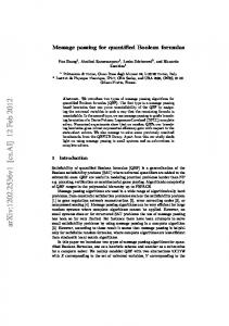
Figure 2: Run-time distributions of SOTA solver for QBFEVAL events. ferent kind of solvers. The above considerations encouraged us to search some new methodologies to improve the stability of AQME P LAIN by devising mechanisms dynamically update the learned policies when they fail to give good results. The result of our research is AQME, a solver that can self-adapt to overcome most of the above problems. The basic consideration when thinking about self-adaptation is that, in order to be effective, such a mechanism has to take into account the run-time distributions of QBF solvers used as basic engines. In order to get an idea about such distributions, we considered the runtime distribution of the SOTA oracle in four QBFEVAL events, from 2004 to 2007. In Figure 2 we plot such runtime distributions in terms of the percentage of problems solved within a given amount of CPU time. In the plot, the x axis is labeled by the CPU time – in seconds on a logarithmic scale; the y axis is the percentage of problems solved within a given time, considering the total number of problems solved within the alloted resources. Each dot is thus a point on the curve describing the empirical runtime distribution of the SOTA oracle in a given QBFEVAL event. Notice that we set the limit on the x-axis scale to 600s, i.e., the time limit used in QBFEVAL’07, in all of our experiments, and also the lowest resource limit used across QBFEVAL events.8 The plot in Figure 2 clearly shows that SOTA oracles, and thus QBF solvers, either manage to evaluate the formulas in a few seconds or they fail even when allowing them several minutes of CPU time. From this observation, we see that there is some margin to design an adaptation schema that fires the predicted engine, but restricting it to a fraction of the available time, and then tries alternative engines, should the predicted one fail to be successful. Whenever an alternative engine is successful, the engine prediction policy can be trained again using the newly acquired information. We call this mechanism retraining. Its main advantages are simplicity, and independence 8 In QBFEVAL’04 and QBFEVAL’05 solvers were limited to 900 seconds of CPU time; in the QBFEVAL’06 marathon track the solvers were limited to 6000s. However, in all such events, the number of formulas solved between 600 seconds and the corresponding time limit is negligible.
18
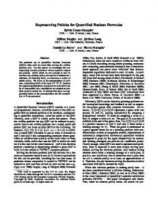
µ, τ , Σ) 1 i ← 0, r ← FAIL 2 while τ > 0 and r = FAIL do 3 σ ← APPLY(µ, ϕ) 4 Σ0 ← REMOVE(Σ, σ) 5 τ 0 ← GAUGE P REDICTED(τ , Σ, i) 6 r ← EXEC(σ, ϕ, τ 0 ), τ ← τ - τ 0 7 while r = FAIL and Σ0 is not empty do 8 hσ, Σ0 i ← REMOVE F IRST(Σ0 ) 9 τ 0 ← GAUGE A LTERNATIVE(τ , Σ, i) 10 r ← EXEC(σ, ϕ, τ 0 ), τ ← τ - τ 0 11 if r 6= FAIL then 12 µ ← UPDATE(µ, ϕ, σ) 13 i←i+1 14 return hr, µi
AQME(ϕ,
Figure 3: Main loop of AQME featuring the retraining algorithm. from the specific inducer used to learn the engine prediction policy. Of course, for retraining to be effective, we should be able to find settings for its parameters – such as, e.g., the resources granted to the engines – that suit different classes of formulas. In order to introduce the study of retraining, in Figure 3 we present the main loop of AQME in pseudo-code format. The function AQME in Figure 3 takes as input four parameters: • ϕ is the QBF to be solved; • µ is an extended inductive model comprised of (i) a classifier that predicts the solver to be run on unseen QBFs, and (ii) a training set, i.e. a set of feature vectors corresponding to QBFs, where each vector is labeled by the best engine on that QBF; • τ is the maximum amount of CPU time granted to solve a single QBF; and • Σ is a list that contains the basic engines of AQME arranged in a specific order. The return value of the function is comprised of the result r, and a – possibly updated – model µ. The result can be one of FAIL, SAT or UNSAT according to whether ϕ could not be solved, was determined to be satisfiable or unsatisfiable, respectively. The algorithm in Figure 3 works as follows: • An iteration counter i and the result r are initially set to 0 and FAIL, respectively (line 1); • The outermost while loop (lines 2 to 13) ends only when either the resources are exhausted, i.e. τ = 0, or when some engine is successful, i.e., r 6= FAIL; notice that the iteration counter i is updated at the end of this loop (line 13). 19
• Inside the main loop, AQME leverages the model µ to predict the best engine σ to be run on the input QBF ϕ; this is the task of the function APPLY (line 3). • The solver σ is removed from the list Σ by the order-preserving function RE MOVE (line 4) to obtain the list of alternative solvers Σ0 ; the function GAUGE P RE DICTED computes a specific time limit τ 0 , possibly considering the amount of resources left τ , the list of engines Σ, and the current iteration i (line 5); • The solver σ is fired on the input QBF ϕ with time limit τ 0 (function EXEC), and the amount of available resources is updated (line 6). • After the call to EXEC, if the result r is either SAT or UNSAT, then the outermost while loop (line 2) ends; otherwise an innermost while loop (lines 7 to 12) starts, and it goes on until either the result r is not FAIL, or there are no more alternative solvers to try, i.e., Σ0 becomes empty; the innermost loop works as follows: – the first solver to try is picked from Σ0 (line 8), and a time limit for such solver is computed by the function GAUGE A LTERNATIVE (line 9), which works analogously to GAUGE P REDICTED. – The alternative solver σ is fired on the input QBF ϕ with time limit τ 0 (function EXEC), and the amount of available resources is updated (line 10); – If the result of the above call is not FAIL, then a call to UPDATE returns an updated model µ (line 11-12); notice that UPDATE must (i) add the feature vector corresponding to ϕ labeled by the currently selected engine σ to the training set stored in µ, and then (ii) swap the classifier stored in µ with a new one obtained considering the updated training set. • AQME returns a pair consisting of the result r and a model µ (line 14); the model µ is unchanged with respect to the input one either when the first predicted engine is successful, or when all the alternatives are unsuccessful. Considering the algorithm described in Figure 3, we can see that by varying the implementations of the “gauge” functions and by sorting in different ways the list Σ, we can control how much time is granted to the predicted engine and to its alternative, as well as how we look for alternatives. These issues are critical for the effectiveness of AQME, so we introduced several variants of both settings. In particular, as far as the implementations of GAUGE P REDICTED and GAUGE A LTERNATIVE are concerned, we considered three different settings: TPE (Trust the Predicted Engine) This is the setting that we hard-wired in the versions of AQME that participated in the QBFEVAL’07 event (see [13]), and it works by allowing a fixed short amount of time to all the engines during the first iteration. Afterwards, should the predicted engine and all the alternative ones be unsuccessful, the whole amount of resources left is granted to the engine predicted in the first place. To see how this works, consider the algorithm in Figure 3 and let L be the initial value of the parameter τ : the function GAUGE P REDICTED and GAUGE A LTERNATIVE should return a value T such that 0 < T < L when 20
i = 0; this can be done because GAUGE P REDICTED “knows” the full amount of resources available when i = 0; during iteration i = 1, if necessary, GAUGE P RE DICTED simply returns τ 0 = τ , i.e., the full amount of resources left. In the version of AQME that competed in QBFEVAL’07 we set T = 10s, where the limit L was 600 seconds. AES (All Engines are the Same) In this setting we grant to all the engines, both the predicted one and the alternative ones, the same amount of CPU time. Still with reference to Figure 3, if L is the initial value of τ , both GAUGE P REDICTED L . Notice that under this setting the and GAUGE A LTERNATIVE return τ 0 = |Σ| outermost while loop spins just one time. ITR (Increasing Time Round-robin) This setting works similarly to AES, in that we always grant to all the engines the same amount of time, but such amount increases in each iteration of the main loop using an exponential progression. Consider Figure 3, and let L be the initial value of τ , and T be some value such that 0 < T L. During iteration i, GAUGE P REDICTED and GAUGE A LTERNATIVE τ return τ 0 = 10i · T unless τ 0 · |Σ| > τ ; in the latter case, τ 0 = |Σ| , i.e., the remaining resources are divided equally among the solvers (as in the AES setting). In all the experiments we run, we set T = 0.1s, so the amount of resources granted to the solvers follows the progression: 0.1, 1, 10, . . .. The rationale behind the three methods is clearly different. In the case of TPE, we are mostly confident in the prediction obtained with the learned model, but we give some chance also to other engines. The setting of T determines how fast an engine needs to be in order to make its way in the model in lieu of the trusted engine. As for AES, we essentially trust all the engines the same. We expect the model to give a relatively good prediction (at least better than flipping a coin), so we try the prediction first. Other than that, the amount of resources granted is the same for all the solvers. Clearly, AES is most effective when the SOTA oracle comprising all the engines can solve all the L given problems within the shared time budget |Σ| . Finally, ITR is also giving all the engines a fair chance, but it is using resources in a more conservative way, trying to solve easy problems without wasting the time budget, and possibly being able to retrain on formulas that are cheaply solved by some engine. The second relevant configuration parameter of AQME is the order in which alternative engines are probed, i.e., how the contents of the list Σ in Figure 3 are sorted. We considered the following settings: RAW The contents of Σ are sorted according to the raw performance results on the QBFEVAL’06, i.e., considering the number of problems solved (higher is better), and, in case of ties, the solution speed (lower is better). YASM The ordering of Σ is the same obtained using the YASM [44] scoring method on the QBFEVAL’06 results. The main difference between YASM and RAW, is that the former takes into account several parameters, including the relative hardness of the formulas, which are not considered when using the latter.
21
ALG The order is based on the kind of engines, i.e., whether they are search-based or hybrid (we introduced the distinction in Section 5). Under this setting, Σ can be supplied to AQME in any order, but R EMOVE F IRST always chooses hybrid (resp. search-based) solvers first, if the predicted solver that failed in the first place was search-based (resp. hybrid). Search-based and hybrid subgroups are ordered using the RAW method. RND Under this setting, the order in which alternative engines are tried is randomly set before the main loop starts. In the following section we will experiment with AQME by combining all the parameter settings described above. One last observation concerns the inductive models that we are going to use. We start by noticing that in AQME the size of the extended model µ at the end of a sequence of runs can be substantially bigger than it was at the beginning. This is because, each time that we update µ, we must also store the feature vector of the QBF that triggered retraining. While the process can stabilize after a while – the more instances we see, the less information we are supposed to be missing – still the amount of time consumed for retraining may jeopardize the effectiveness of the whole retraining schema, and we may end up consuming more time to train the models rather than to solve QBFs. For all the inducers that we considered in AQME, the balance between training time, and the growing size of the training set is favorable, except in the case of MLR. As some preliminary experiments with AQME show, the training time of MLR grows too high after a relatively small number of retrainings, so we decided to drop this inducer in the experimentation that follows.
8
Experimental evaluation of AQME
This section consists of two parts. In the first one, we try to understand which are the combinations of settings introduced in the previous section that yield the best performances. In the second part, we test the best combination of settings on the QBFEVAL’07 dataset by comparing AQME with AQME P LAIN and the competitors of QBFEVAL’06/07. Unless specified otherwise, all the experiments we show are carried out using the platform outlined in Section 5, and the engines are limited to 600s of CPU time, and 900MB of main memory.
8.1
Tuning the adaptive component
Table 10 (Appendix B) shows the results of our first experiment with AQME. Here we tested all the combinations (36) of the factors that can influence its performances, namely the resource allocation strategy (one of TPE, AES, and ITR), the engine order (one of RAW, YASM, ALG, RND), and the inductive model used (either C4.5, 1NN, or R IPPER). The data corresponding to the RND setting are obtained by considering the median values over 100 runs, each one time considering a different random sample of the engine order.
22
Considering the data in Table 10, and bearing in mind that the SOTA oracle built out of the basic engines in AQME can solve 636 problems on this dataset, we can conclude the following: • The performance data of AQME are relatively independent from the inducer; this phenomenon is particularly evident when considering the number of problems solved and the AES settings, but we can see that the worse combination (RND+TPE+1NN) can solve “only” 18 problems less than the best combinations (any of the ones with AES). • Overall, AQME is strikingly better than AQME P LAIN: the former solves 570 problems in the worst case, while the latter solves 486 problems in the best case, nearly 90% versus 75% of the problems that can be solved by the SOTA oracle; moreover, the combination yielding AQME best case – topping at 92% of the problems solved by the SOTA oracle – is independent of the specific inducer, while in the case of AQME P LAIN changing the inducer can have dramatic effects. • When considering the number of problems solved, changing the order in which solvers are tried does not matter much, particularly in the AES setting; however choosing a “good” ordering does have an effect on performances; in terms of solution speed, while RAW and YASM are always better than RND, the ALG setting is less robust. • AES turns out to be the best method to allocate resources; this is true independently from the inductive model, although slightly better performances can be obtained using C4.5, mainly because this inducer strikes a good balance between classification and training speed. When analyzing the above results it is useful to consider that the SOTA oracle comprised of AQME engines is indeed able to solve every formula in the QBFEVAL’07 dataset within 75s of CPU time, which is the maximum amount of time that each engine is granted under the AES setting. If we consider that during the last iteration of ITR all the engines are granted about 65 seconds, we see that the slightly weaker performances of ITR with respect to AES are mostly explained by the fact that some of the hardest formulas could not be solved within the reduced time limit. The above considerations call for two points to be addressed. First, we would like to understand what happens when a non negligible number of the problems cannot be L solved within |Σ| . This can be done, e.g., by reducing the time budget alloted to AQME and repeating the above experiments. Second, it is also interesting to assess the cost of exploring alternative reasoners and updating the model. This can be done, e.g., by rerunning AQME using the model on the very same dataset on which AQME adapted itself. To understand the impact of a reduced initial time budget on AQME, we considered a time limit of 100s instead of 600s. The number of problems that cannot be solved L within |Σ| is now substantially higher, so we expect a different behavior of AQME. Table 11 (Appendix B) shows the results of such experiment, from which we can see that TPR and ITR – with the latter being slightly better than the former – are now both outperforming AES. The advantage of TPR and ITR over AES is not sensitive to the
23
ordering of Σ, although the relative performance of TPR versus ITR is so. Overall this indicates that under stress conditions, methods that make a more conservative use of the time budget may have an edge over other approaches. To assess the cost of adaptation in AQME, we considered the final model learned by AQME as the initial one, and the we re-run the experiments on the same dataset. Table 12 (Appendix B) shows the results of such experiment, from which we can see that the time spent for exploring alternative engines and for updating the model is a relevant portion of the total runtime of AQME. In particular, the AES setting enables us to get a very precise estimate, since it is the only one in which using the final model does not increase the number of problems solved. Looking at the AES setting only, and considering AQME total time as shown in Table 10, we can see that adaptation time goes from a minimum of 44% for AQME 1NN (YASM) to a maximum of 77% for AQME -1NN (ALG), with an average of 58%. In other words, about half of the total time of AQME is spent, on average, for exploring alternative solvers and updating the internal models. In order to investigate the difference in performances between the various settings that we tried, in Table 13 (Appendix B) we report data concerning the retraining effects on the inducer predictions. From Table 13, we can conclude that under all the engine orderings and for all the inducers, TPE is the setting that triggers the least number of retrainings, while AES is the one that triggers the most – with the exception of C4.5+AES+ALG and R IPPER+AES+ALG. If we compare this with the data in Table 10, we see that for AQME to be effective, the right balance must be struck between exploitation of the current model and exploration of alternatives. While a high number of retrainings can be expensive and can make the model unstable, a small number of them may not allow the model to self-adapt effectively. According to our data, it seems that AES gets the balance right, even if it has an overall smaller number of correct predictions than TPE and ITR. One last observation about Table 13 is that, considering the AES setting, C4.5 is the inducer that shows the highest number of correct predictions, over all possible engine orderings. These data suggests that C4.5 seems to be the inducer which can take better advantage of retraining. Finally, Table 14 (Appendix B), shows further data to see how the engine ordering affects AQME under various settings, particularly when considering how many engines AQME must try before finding one that can actually solve the formula at hand. If we consider the distributions of the engine trials, we see that for TPE and AES settings each such distribution has as many elements as the number of retrainings reported in Table 13. The range of such distributions is between one – AQME retrains itself on the first solver selected when the prediction fails – and 7 – AQME retrains itself on the last solver tried. As for ITR, we can see that the range extends beyond 7, since it is possible that the engines fail to solve formulas within short time limits, and this may happen for several rounds – at most 4 in our setup. The results presented in Table 14 show that the number of engine trials are pretty much the same across various engine orderings, while the resource allocation schema influences them more heavily. Considering, for instance, AQME -1NN, we see that the median number of engines tried is 2, when considering TPE and AES settings under RAW and YASM orderings. This means that when a prediction fails, AQME needs to evaluate 2 engines on average, before being able to retrain itself. Considering ALG and RND orderings the same value raises to 4 and 3, respectively. Since the above considerations are true for all the inducers, this 24
Solver AQME -C4.5 AQME -R IPPER AQME -1NN Q U BE5.0? AQME P LAIN -MLR NC Q U BE 1.0 NC Q U BE 1.1 S K IZZO QCK AQME P LAIN -1NN S K IZZO STD Q U BE3.0? S K IZZO ? AQME P LAIN -C4.5 2 CLS Q? AQME P LAIN -R IPPER SSOLVE? A DAPTIVE 2 CLS Q QUANTOR ? QUANTOR 2.15 Y Q UAFFLE Y Q UAFFLE ? QUAFFLE? SQUOLEM EBDDRES
Table 4: AQME and AQME P LAIN versus their engines and QBFEVAL’07 contestants. provides also an explanation about the fact that RAW and YASM orderings tend to perform better than ALG and RND orderings.
8.2
Testing AQME on the QBFEVAL’07 dataset
In Table 4, we report a comparison among AQME P LAIN, AQME, their engines and the QBFEVAL’06 contestants. AQME is configured using the AES+RAW combination of settings. The solvers that we used as engines are marked with a “?” to distinguish them from the QBFEVAL’07 contestants, some of which are newer versions of the same solver. Table 4 is structured similarly to Table 2 where for each engine we report the number of formulas solved (“#”) and the cumulative CPU time to solve them (“Time”). As we can see from Table 4, AQME is a clear improvement over AQME P LAIN. First, AQME is able to solve 20% formulas more with respect to AQME P LAIN. Second, and even more important, the performance of AQME is stable across different inducers, while this was not the case for AQME P LAIN. We conjecture that, as long as an inducer can be trained reasonably quickly, using retraining should guarantee good performances independently from the specific model adopted. Notice that AQME is faster than all its engines and all QBFEVAL’07 contestants as well, which means that using a self-adaptive multi-engine solver can effectively improve the performances over the current state-of-the-art solvers.
25
9
Conclusions
In this paper we have studied the problem of engineering a robust solver for QBFs. In particular we have shown that we can obtain a tool capable of effectively solving formulas in different problem domains without the need for domain-specific tuning. We have showed that a set of inexpensive syntactic features can hint the best solver to run on each QBF, and that harnessing inductive reasoning techniques leads to effective engine-selection policies. AQME P LAIN, our basic multi-engine solver, can choose among its engines the one which is more likely to yield optimal results, it is more robust than each single engine, and it is also stable with respect to various perturbations applied to the training/test sets. In order to improve on AQME P LAIN, we investigated the possibility of updating the learned policies when they fail to give good predictions. The result of our study is AQME, a multi-engine solver that is also self-adaptive, i.e., able to improve itself when the usage scenario changes substantially. Our experiments confirmed that the retraining algorithm can be optimized for a wide class of formulas, and that AQME can be more robust and efficient than state-of-the-art single-engine solvers, even when it is confronted with formulas and competitors which were not used for engineering it. This work advances the state of the art in QBF by proposing a novel way of combining existing solvers that is more efficient and robust than the best currently available solvers.
Acknowledgements We wish to thank the Italian Ministry of University and Research for its financial support. We would like to acknowledge all the researchers submitting their work to QBFLIB and QBFEVAL, since without their efforts this work would not have been possible. Enrico Giunchiglia and Massimo Narizzano are to be thanked for helpful discussions and feedback on early drafts of this paper. Finally, we wish to thank the anonymous reviewers for giving us helpful suggestions on how to improve the draft version of the paper.
References [1] L. J. Stockmeyer and A. R. Meyer. Word problems requiring exponential time. In 5th Annual ACM Symposium on the Theory of Computation, pages 1–9, 1973. [2] C. H. Papadimitriou. Computational Complexity. Addison-Wesley, 1994. [3] I.P. Gent, P. Nightingale, and A. Rowley. Encoding Quantified CSPs as Quantified Boolean Formulae. In Proceedings of the 16th European Conference on Artificial Intelligence (ECAI 2004), pages 176–180, 2004. [4] M. Mneimneh and K. Sakallah. Computing Vertex Eccentricity in Exponentially Large Graphs: QBF Formulation and Solution. In Sixth International Conference on Theory and Applications of Satisfiability Testing (SAT 2003), volume 2919 of Lecture Notes in Computer Science, pages 411–425. Springer Verlag, 2003. 26
[5] Z. Hanna N. Dershowitz and J. Katz. Bounded Model Checking with QBF. In Eight International Conference on Theory and Applications of Satisfiability Testing (SAT 2005), volume 3569 of Lecture Notes in Computer Science, pages 408– 414. Springer Verlag, 2005. [6] T. Jussila and A. Biere. Compressing BMC Encodings with QBF. In Proc. 4th Intl. Workshop on Bounded Model Checking (BMC’06), 2006. [7] Jussi Rintanen. Partial implicit unfolding in the Davis-Putnam procedure for Quantified Boolean Formulae. In Proc. LPAR, volume 2250 of LNCS, pages 362– 376, 2001. [8] H. Turner. Polynomial-length planning spans the polynomial hierarchy. In In Proc. of Eighth European Conf. on Logics in Artificial Intelligence (JELIA’02), volume 2424 of Lecture Notes in Artificial Intelligence, pages 111–124. Springer Verlag, 2002. [9] C. Castellini, E. Giunchiglia, and A. Tacchella. SAT-based planning in complex domains: Concurrency, constraints and nondeterminism. Artificial Intelligence, 147:85–117, 2003. [10] C. Ansotegui, C.P. Gomes, and B. Selman. Achille’s heel of QBF. In Proc. of AAAI, pages 275–281, 2005. [11] U. Egly, T. Eiter, H. Tompits, and S. Woltran. Solving Advanced Reasoning Tasks Using Quantified Boolean Formulas. In Seventeenth National Conference on Artificial Intelligence (AAAI 2000), pages 417–422. The MIT Press, 2000. [12] Guoqiang Pan and Moshe Y. Vardi. Optimizing a BDD-based modal solver. In Proceedings of the 19th International Conference on Automated Deduction, volume 2741 of Lecture notes in Computer Science, pages 75–89. Springer Verlag, 2003. [13] M. Narizzano, L. Pulina, and A. Taccchella. QBF solvers competitive evaluation (QBFEVAL), 2006. http://www.qbflib.org/qbfeval. [14] B.A. Huberman, R.M. Lukose, and T. Hogg. An economics approach to hard computational problems. Science, 3, 1997. [15] E. Nudelman, A. Devku, Y. Shoham, and K. Leyton-Brown. Understanding Random SAT: Beyond the Clauses-to-Variables Ratio. In 10th Int.l Conference on Principles and Practice of Constraint Programming (CP2004), volume 3258 of LNCS, pages 438–452. Springer-Verlag, 2004. [16] L. Xu, H.H. Hoos, and K. Leyton-Brown. Hierarchical Hardness Models for SAT. In 13th Conference on Principles and Practice of Constraint Programming (CP 2007), volume 4741 of Lecture Notes in Computer Science, pages 696–711. Springer Verlag, 2007.
27
[17] J. R. Quinlan. C4.5: Programs for Machine Learning. Morgan Kaufmann Publishers, 1993. [18] William W. Cohen. Fast effective rule induction. In Twelfth International Conference on Machine Learning., pages 115–123, 1995. [19] S. Le Cessie and J.C. van Houwelingen. Ridge estimators in logistic regression. Applied Statistics., 41:191–201, 1992. [20] D. Aha and D. Kibler. Instance-based learning algorithms. Machine Learning, pages 37–66, 1991. [21] C.P. Gomes and B. Selman. Algorithm portfolios. Artificial Intelligence, 126:43– 62, 2001. [22] E. Nudelman, K. Leyton-Brown, A. Devkar, Y. Shoham, and H. Hoos. SATzilla: An Algorithm Portfolio for SAT. In In Seventh International Conference on Theory and Applications of Satisfiability Testing, SAT 2004 Competition: Solver Descriptions, pages 13–14, 2004. [23] L. Xu, F. Hutter, H.H. Hoos, and K. Leyton-Brown. The Design and Analysis of an Algorithm Portfolio for SAT. In 13th Conference on Principles and Practice of Constraint Programming (CP 2007), volume 4741 of Lecture Notes in Computer Science, pages 712–727. Springer Verlag, 2007. [24] D. G. Mitchell, B. Selman, and H. J. Levesque. Hard and Easy Distributions for SAT Problems. In Proceedings of the Tenth National Conference on Artificial Intelligence, pages 459–465. AAAI Press, 1992. [25] L. Pulina and A. Tacchella. A multi-engine solver for quantified boolean formulas. In 13th Conference on Principles and Practice of Constraint Programming (CP 2007), volume 4741 of Lecture Notes in Computer Science, pages 574–589. Springer Verlag, 2007. [26] H. Samulowitz and R. Memisevic. Learning to Solve QBF. In In proc. of 22nd Conference on Artificial Intelligence (AAAI’07), pages 255–260, 2007. [27] C. Gebruers, B. Hnich, D.G. Bridge, and E.C. Freuder. Using CBR to Select Solution Strategies in Constraint Programming. In Proceedings of the 6th Int.l Conf. of Case-Based Reasoning, Research and Development (ICCBR 2005), pages 222– 236, 2005. [28] L. Lobjois and M. Lemaˆıtre. Branch and Bound Algorithm Selection by Performance Prediction. In Proceedings of 15th Nat.l Conf. on Artificial Intelligence (AAAI 1998), pages 353–358, 1998. [29] M.J. Streeter, D. Golovin, and S.F. Smith. Restart Schedules for Ensembles of Problem Instances. In Proceedings of 22nd AAAI Conference on Artificial Intelligence (AAAI 2007), pages 1204–1210, 2007.
28
[30] E. Giunchiglia, M. Narizzano, and A. Tacchella. Quantified Boolean Formulas satisfiability library (QBFLIB), 2001. www.qbflib.org. [31] M. Narizzano and A. Tacchella. QDIMACS prenex CNF standard ver. 1.1, 2005. Available on-line from http://www.qbflib.org/qdimacs.html. [32] M. Davis, G. Logemann, and D. Loveland. A machine program for theorem proving. Communications of the ACM, 5(7):394–397, 1962. [33] H. Kleine-B¨uning, M. Karpinski, and A. Fl¨ogel. Resolution for Quantified Boolean Formulas. Information and Computation, 117(1):12–18, 1995. [34] M. Benedetti. sKizzo: a Suite to Evaluate and Certify QBFs. In 20th Int.l. Conference on Automated Deduction, volume 3632 of Lecture Notes in Computer Science, pages 369–376. Springer Verlag, 2005. [35] A. Biere. Resolve and Expand. In Seventh Intl. Conference on Theory and Applications of Satisfiability Testing (SAT’04), volume 3542 of LNCS, pages 59–70, 2005. [36] M. Narizzano, L. Pulina, and A. Tacchella. The third QBF solvers comparative evaluation. Journal on Satisfiability, Boolean Modeling and Computation, 2:145– 164, 2006. Available on-line at http://jsat.ewi.tudelft.nl/. [37] M. Narizzano, L. Pulina, and A. Tacchella. The QBFEVAL Web Portal. In 10th European Conference on Logics in Artificial Intelligence (JELIA 2006), volume 4160 of Lecture Notes in Computer Science, pages 494–497. Springer Verlag, 2006. [38] I. St´ephan. Boolean Propagation Based on Literals for Quantified Boolean Formulae. In Proceedings of 17th European Conf. on Artificial Intelligence (ECAI 2006), pages 452–456, 2006. [39] I.H. Witten and E. Frank. Data Mining (2nd edition). Morgan Kaufmann, 2005. [40] L. Kaufman and P.J. Rousseeeuw. Finding Groups in Data. Wiley, 1990. [41] M. Herbstritt, B. Becker, and C. Scholl. Advanced SAT-Techniques for Bounded Model Checking of Blackbox Designs. In MTV workshop, pages 37–44, 2006. [42] I.P. Gent and A.G.D. Rowley. Encoding Connect 4 using Quantified Boolean Formulae. Technical Report APES-68-2003, APES Research Group, July 2003. [43] Ron Kohavi. A study of cross-validation and bootstrap for accuracy estimation and model selection. In In Proc. of Int.l Joint Conference on Artificial Intelligence (IJCAI), pages 1137–1145, 1995. [44] M. Narizzano, L. Pulina, and A. Tacchella. Ranking and Reputation Sytems in the QBF competition. In 10th Conference of the Italian Association for Artificial Intelligence (AI*IA 2007), volume 4733 of Lecture Notes in Artificial Intelligence, pages 97–108. Springer Verlag, 2007. 29
A
QBF features
Basic features • c, total number of clauses; c1 , c2 , c3 total number of clauses with 1, 2 and more than two existential literals, respectively; ch , cdh total number of Horn and dual-Horn clauses, respectively; • v, total number of variables; v∃ , v∀ , total number of existential and universal variables, respectively; ltot , total number of literals; vs, vs∃ , vs∀ , distribution of the number of variables per quantified set, considering all the variables, and focusing on existential and universal variables, respectively; s, s∃ , s∀ , number of total, existential and universal, quantified sets; • l, distribution of the number of literals in each clause; l+ , l− , l∃ , l∃+ , l∃− , l∀ , l∀+ , l∀− , distribution of the number of positive, negative, existential, positive existential, negative existential, universal, positive universal, negative universal number of literals in each clauses, respectively. • r, distribution of the number of variable occurrences r+ , r− , r∃ , r∃+ , r∃− , r∀ , r∀+ , r∀− , distribution of the number of positive, negative, existential, positive existential, negative existential, universal, positive universal, negative universal variable occurrences, respectively; wr, wr+ , . . . (as above), distributions of the number of variable occurrences weighted according to prefix level.
Combined features • p, distribution of the values of the products, computed for each existential variable x, between the number of occurrences of x and the number of occurrences of ¬x; wp, the same as p, where each product is weighted according to the prefix level. •
c , v
the classic clauses-to-variables ratio, and for each x ∈ {l, r, wr} the following ratios (on mean values): – – –
•
B
x+ x− x+ , x , x− , x
balance ratios;
x∃ x∃+ x∃− x∃+ x∃− x∃+ , x , x , x∃ , x∃ , x∃− , x x∀ x∀+ x∀− x∀+ x∀− x∀+ , x , x , x+ , x− , x∀ , x
Max 78971 34659 13063 27363 18742 1832 6967 131072 178750 3877 c Med 19381 22865.5 150266 19954.5
c Med 28140 4480.5 2764 15588 10648 560.5 2665 3274 3568 3646.5
Table 5: QBFEVAL’06/07 datasets synopses: “#” is the number of formulas per suite, and the remaining columns are the statistics – (Min)imum, (Med)ian, and (Max)imum – regarding the number of existential (v∃ ), and universal (v∀ ) variables, the number of quantified sets (s), the number of clauses (c) and the total number of literals (ltot ).
QBFEVAL’07 Suite Biere Herbstritt Mangassarian-Veneris Palacios
QBFEVAL’06 Suite Ansotegui Ayari Biere Gent-Rowley Herbstritt Ling Mneimneh-Sakallah Pan Rintanen Scholl-Becker
Table 6: Estimating the performances of AQME P LAIN 2, AQME P LAIN 16 and AQME P LAIN 8 (column “Version”). Column “CV” is the fold index, and column “N” is the number of QBFs in the fold. The first four groups of two columns report estimates of AQME P LAIN performances: (i) the number of formulas solved (column “#”), and (ii) the cumulative CPU time of AQME P LAIN (column “Time”). The group “Best” contains measures (i) and (ii) computed for the best single-engine on the specific fold. The column “SOTA” contains measure (ii) computed for the SOTA solver. The “Overall” rows refer to the mean ratio of problems solved (column “#”), and the median CPU time (column “Time”).
Table 7: Results obtained by randomly choosing datasets for training that decrease in size. The first column contains the solver names, and it is followed by five groups of columns, one for each percentage of removed instances, with an indication of the cardinality of the test set. For instance, when removing 10% of the instances from the dataset (first group of columns), we are left with a test set numbering 32 formulas. The two subgroups “B” (resp. “W”) show the best (resp. worst) case performances of each solver across 50 test sets samples obtained by removing a specific percentage of formulas from the original QBFEVAL’06 dataset. The columns “#” and “Time” contain, respectively, the number of formulas solved and the cumulative CPU seconds – including the default time limit value for the formulas that could not be solved using the allotted resources. The top-three performers in each subgroup are highlighted with bold text. In case of ties in the number of problems solved, the solver yielding the smallest time is preferred.
Table 8: Results obtained by choosing increasingly easier datasets for training. The table is arranged similarly to Table 7, modulo the fact that best- and worst-case performances coincide, since the test sets are obtained deterministically.
QUANTOR SSOLVE Y Q UAFFLE QUAFFLE
C4.5 1NN MLR R IPPER Q U BE5.0 2 CLS Q S K IZZO Q U BE3.0
Table 9: Results obtained by biasing the dataset used for training in favor of a given solver. The first column contains the solver names, and it is followed by eight group of columns, one for each engine of AQME P LAIN whereupon the training set is biased. The number of instances in each of the eight test sets is (from left to right): 96, 202, 138, 197, 121, 104, 146, and 204. The table is then arranged as Table 8. When the training set is biased in favor of a given solver, a dash indicates that the corresponding test set does not contain any formula that can be evaluated by such solver within the allotted resources.
Y Q UAFFLE
AQME P LAIN -C4.5 AQME P LAIN -R IPPER AQME P LAIN -MLR 2 CLS Q QUAFFLE QUANTOR Q U BE3.0 Q U BE5.0 S K IZZO SSOLVE
Table 12: The same experiment of Table 10, using the adapted model.
AES Time 5531 9913 6713 10914
AQME -1NN
# 588 588 588 588
AES Time 8227 9739 16154 14227
AQME -R IPPER
ITR Time 10699 8497 12025 17232
ITR Time 5801 6054 7179 7422
# 582 584 584 584
Table 11: The same experiment of Table 10, using a time limit of 100 seconds instead of 600 seconds.
TPE # Time 533 3196 533 3127 532 4287 533 4226
Table 10: Experimental results of AQME under a combination of factors: resource allocation strategy (one of TPE, AES, and ITR), engine order (one of RAW, YASM, ALG, RND), and inductive model used (either C4.5, 1NN, or R IPPER). For each combination, the table reports the number of problems solved (“#”) and the cumulative CPU time consumed to solve them (“Time”) – including the default time limit for the formulas that could not be solved, and the overhead of updating the engine selection policies.
RAW YASM ALG RND
# 576 572 572 570
TPE Time 15392 14384 14947 19438
37
R 35 33 33 39
C 513 513 506 504
AES R 75 75 82 84
AQME -1NN
C 520 520 520 515
ITR R 65 65 65 69
C 533 527 534 523
TPE R 40 46 47 52
C 518 518 525 514
AES R 70 70 63 74
AQME -C4.5
C 526 523 518 517
ITR R 59 60 67 67
C 546 536 538 528
TPE R 28 34 35 44
AES C R 514 74 515 73 508 80 502 86
AQME -R IPPER
ITR C R 502 78 493 87 502 80 496 87
RAW YASM ALG RND RAW YASM ALG RND RAW YASM ALG RND
Table 14: Number of engines evaluated by AQME when the predicted engine fails. AQME versions are grouped by row and, for each combination of settings, we report the minimum (“Min”), the median (“Med”) and the maximum (“Max”) value obtained considering the distributions of the number of unsuccessful trials before finding a good candidate for retraining. Data about the RND setting are median values among 100 samples. For TPE and AES settings, each distribution has as many elements as the number of retrainings reported in Table 13. The range of such distributions is between one – AQME retrains itself on the first solver selected when the prediction fails – and 7 – AQME retrains itself on the last solver tried. As for ITR, it is possible that all the engines fail to solve formulas within short time limits, and this may happen for several rounds – at most 4 in our setup.
AQME -R IPPER
AQME -C4.5
AQME -1NN
Min 1 1 1 1 1 1 1 1 1 1 1 1
Table 13: Number of correct predictions vs. number of retrainings in AQME on the QBFEVAL’07 dataset. The table is arranged in the same way as Table 10, where for each combination of settings, we report the number of times in which the predicted solver was able to solve the input QBF (“C”), versus the number of times in which retraining was triggered (“R”).