A spiking neural sparse distributed memory implementation for learning and predicting temporal sequences J. Bose, S. B. Furber, and J. L. Shapiro School of Computer Science, University of Manchester,Manchester, UK, M13 9PL.
[email protected], [steve.furber,jonathan.shapiro]@manchester.ac.uk
Abstract. In this paper we present a neural sequence machine that can learn temporal sequences of discrete symbols, and perform better than machines that use Elman’s context layer, time delay nets or shift register-like context memories. This machine can perform sequence detection, prediction and learning of new sequences. The network model is an associative memory with a separate store for the sequence context of a pattern. Learning is one-shot. The model is capable of both off-line and on-line learning. The machine is based upon a sparse distributed memory which is used to store associations between the current context and the input symbol. Numerical tests have been done on the machine to verify its properties. We have also shown that it is possible to implement the memory using spiking neurons.
1
Introduction
Time is important in many real world tasks. Many applications are sequential in nature, where the time order of events is important. A sequence machine is a system capable of storing and retrieving temporal sequences of patterns that represent discrete symbols. Neural models of temporal sequence learning have been a source of interest [7, 1, 2]. We are interested in a model that does one-shot learning, can learn on-line, has good memory capacity, can work with a variety of sequences and can be implemented using spiking neurons. We do not feel a model with all these features has been developed earlier.
2
Sequence learning
One thing we need to consider is that two different sequences may have certain symbols in common. If we use an associative memory to learn the two sequences, where the association is between the current symbol and the next symbol, it cannot decide the next symbol after the common because the two sequences have different successors of the common symbol. It needs to have some idea of the context as well. Thus the basic sequence machine needs to have four
Input
Input
ip
Previous Context
ip(t)=input at time t
ip(t−1) Context
context
Associative
Layer
Associative Context
Memory
Memory ip(t−2)
Shift Register Context Output Output (a)
(b)
Fig. 1. (a)Shift register model and (b)a separate neural layer as context
components: input, output, main memory and context memory. The ideal online sequence machine is one that can look back from the most recent inputs, as far as is necessary to find a unique context for deciding the next character to be predicted. The machine should be able to ‘lock-on’ or converge to a context (and thus predict the next output) if it has seen it earlier, and to learn the new association if it has not. It should have infinite look-back, yet should be able to distinguish between different contexts. When a new symbol is presented at the input of the on-line sequence machine, first of all it learns to associate the new input symbol with the present value of the context. Based on the new input and the present context, it creates a new context. Finally it predicts the next output by presenting the modified context to the memory. The above steps incorporate both prediction and learning. If the memory has seen a similar input and context before, the expected next output will be predicted. On the other hand, if it is given a new association, it writes it to the memory. In this case the predicted output will be erroneous, but the new association written into the memory should improve its performance if a similar context is encountered subsequently. 2.1
The Shift Register model
One way to represent the context could be to have a fixed length time window of the past, and associate the next output with inputs in the time window, as is done in Time Delay Neural Nets (TDNN)[6]. Such a memory acts like a shift register. However, the time window is of fixed size, and the number of common symbols might be greater than this. Fig. 1(a) shows a shift register with lookback of 2. 2.2
The context neural layer model
Another approach is to use a separate ‘context’ neural layer, with fixed weights, to represent the entire history of the sequence. Fig. 1(b) gives the structure of the
1 0 0 1 0 1 0 1 0 1 0 1
Letter Sequence
Input Letter
Old context
N of M encoder
N of M code
Input
Scramble Deterministically (simulates neural layer)
Prev.cxt
Expand
Data Store
Address Decoder
Context
Expand
+
N of M SDM
Sequence Machine N of M code
Contract N of M decoder
(a)
1 0 0 1 0 1
Output Letter
(b)
New context
Fig. 2. (a) shows a sequence machine using an N-of-M Kanerva SDM, having address decoder, data memory and context neural layers. (b) shows how the new context is created from the old context and the input in the combined model. The model has aspects of both the neural layer and the shift register.
context layer based model. The influence of the old context can be modulated by multiplying the old context outputs by a constant λ and feeding them back as inputs. The context encodes the entire past history or ‘state’ of the sequence. Such a model resembles a finite state machine. A similar model with feedback was used by Elman [4]. A problem with the context neural layer model is that to retrieve a sequence we need to start retrieval from the beginning, else the context will be different.
2.3
Combined model
The shift register model and the separate context layer model both have their advantages and disadvantages. We combine the two in a new memory model by using a separate context layer with modulated context, where the new context is determined by both the input and a shifted version of the present context. The new context is formed from the input and old context as follows (see fig. 2(b)): First we scramble of the old context, which is equivalent to passing it through a neural layer. Then the old context is mapped on to a high dimension, expanded and added to the expanded input. The sum is then contracted. The intention is that the result should be strongly dominated by the present input, but should have some bits of the past context in it as well.
100 100
Combined model Neural layer Shift register
80
90
No of symbols predicted correctly
No of symbols predicted correctly
90
70
60
50
40
30
20
10
lambda=1.0 lambda=0.9 lambda=0.7 lambda=0.5 lambda=0.3 lambda=0.2 lambda=0.1 lambda=0
80
70
60
50
40
30
20
10
(a)
10
20
30
40
50
60
70
Length of input sequence
80
90
100
(b)
10
20
30
40
50
60
70
80
90
100
Length of input sequence
Fig. 3. (a) compares the performance of three types of sequence memories: Shift register, neural layer and the combined model. The straight line represents the ideal case, when the complete sequence is recovered. The combined model(dotted line) performs better than the others.(b) shows the memory capacity of the combined model in which the context sensitivity λ has been varied to see what effect λ has on memory performance. The topmost curve is for λ=1.0 and lowest for λ=0
3
An implementation using sparse distributed memory
We implemented the sequence machine using a modified Kanerva Sparse Distributed Memory (SDM)[3] using N-of-M codes[5]. We used an N-of-M code to encode the symbols, in which N of a total M components are active simultaneously to give a valid code. Such memories have been shown to have good information efficiency, scalability and error tolerance[5]. The N-of-M SDM has two layers of neurons: an address decoder layer, whose primary purpose is to cast the input symbols into high dimensional space to make it linearly separable, and a second correlation-matrix layer called the data store, which associates the first symbol as decoded by the first neural layer, with the second symbol. Learning takes place only in this layer, while the weights of the first address decoder layer are set to a constant random value. The complete system with context is shown in fig. 2(a).
4
Numerical tests on the sequence machine
We conducted some tests on the sequence machines described above, to compare their behaviour with different kinds of sequences. There are three kinds of sequence machine we are comparing, namely the shift register, context neural layer and combined model. In each case we used the same SDM of size 512 by 256, with 1024 address decoder neurons. Each input symbol was encoded as an ordered 11-of-256 code vector. The learning algorithm used in the data store of the SDM is that the new weight matrix is formed by taking the maximum of the old weight matrix and the outer product of the two vectors that are being associated. Comparison of different models: Here we compare the three models of sequence machine with optimised parameters and analyse their memory capacity for different sequence lengths. Repeated characters are guaranteed for sequence
Initial dispersion is 0
6
5
4.5
5
Avg dispersion (over 15 runs)
THRESHOLD
Activation Value
4
3
2
1
0
4
3.5
3
2.5
2
1.5
1
−1 0.5
(a)
−2
0
10
20
30
40
Time
50
60
70
80
(b)
0
0
20
40
60
80
100
120
140
160
180
200
Layer no.
Fig. 4. (a) is the plot of a typical neural activation with time, when the neuron receives a single input spike at t=0. (b) plots the average dispersion over 16 runs of a burst of spikes over a network of 200 feed-forward layers.
length greater than 15, which is the alphabet size. Figure 3(a) shows the results. For each point on the figure we started with a blank memory and input the sequence twice. The memory learns the sequence on the first presentation of the input, and in the second time we check the predicted output sequence to see how accurate the prediction is. We see that the combined model performs the best of the three and obtains near perfect recall. Effect of the context sensitivity factor: Here we vary the context sensitivity factor λ and see the memory performance of the combined model. We see three clear zones. When lambda is 0, the machine is not at all sensitive to context and it performs badly. When it is 1, which means that the context is given equal priority as the current input, it performs quite well, giving near perfect matching. When it is between these two zones, the combined model behaves effectively like a shift register. Fig. 3(b) shows one such experiment.
5
Implementation issues using spiking neurons
In this section we mention a few issues when implementing this sequence machine using low level asynchronous spiking neurons. One of the reasons we used SDM’s to create our memory was their suitability to spiking neural implementation. We define a symbol in our sequence machine as being represented by a burst of spikes emitted by a layer of neurons, the information being encoded in the choice of neurons firing and times of firing. When modelling such high level synchronous systems using low level components, we need to ensure that the stability and coherence of the symbols is maintained. By stability we mean that the spike burst should not either die out or saturate when propagated through different layers, but maintain the same average level. By coherence we mean that the different bursts should not interfere with each other, else it would destroy the information being propagated as symbols. For our modelling we used a modification of the standard leaky integrate and fire (LIF) neural model [8], in which incoming spikes increment the driving force or first derivative of the activation, rather than the activation itself. Like in the
standard model, if the activation exceeds a local threshold, the neuron fires a spike and the activation and the driving force are reset. Both the activation and the driving force decay with time, the rates of decay being governed by their respective time constants. Fig. 4(a) shows the shape of the activation curve following a single input spike at time 0. We see that the activation at first increases due to the increased driving force caused by the incoming spike, but after a time the decay becomes dominant. There is an inherent time lag between the input spike and the maximum activation reached by the neuron. If the system contains a feedback loop, such a time lag is necessary, or else at least one input neuron would have to fire a spike at the same time as an output neuron fires a spike, and there would be no temporal separation between the input and output bursts. The standard LIF model cannot achieve this property. This motivated our choice of neural model. We then simulated a network of 200 feed forward layers with same average connectivity but random connection weights. We gave the first layer a random input spike burst of firings, and propagated the output burst to the successive layers. We ensured that the bursts were stable through feedback reset inhibition. We then plotted the temporal separation of the bursts in each layer. The results of one such experiment are plotted in fig. 4(b). We see that the average burst width tends to settle around a narrow time range. If we ensure that the separation between different bursts is large compared to this average time of one burst (by adding extra delays), we can prevent different spike bursts from interfering. This shows it is possible for a spike burst to maintain coherence. So by tuning the delays between the bursts it is possible to implement the sequence machine using spiking neurons.
6
Conclusions and further work
We have developed a model that is capable of on-line sequence learning and prediction. More work needs to be done on issues of implementation by real time spiking neurons. Work also needs to be done to develop suitable applications.
References 1. Vocal interface for a man-machine dialog. Dominique Beroule. ACL Proceedings, First European Conference, 1983. 2. Learning Speech as Acoustic Sequences with the Unsupervised Model, TOM. S. Durand and F. Alexandre. NEURAP, 8th Intl. conference on neural networks and their applications, France, 1995. 3. P. Kanerva. Sparse Distributed Memory. MIT Press, 1988 4. J. L. Elman. Finding structure in time. Cognitive Science, 1990, 14. 5. S.B. Furber, J.M. Cumpstey, W.J. Bainbridge and S. Temple. Sparse distributed memory using N-of-M codes. Neural Networks. 2004, 10 6. K.J. Lang and G. E. Hinton. The development of the time delay neural network architecture for speech recognition. Tech.Report 88152, Carnegie Mellon, 1988. 7. R. Sun and C.L. Giles (Eds.) Sequence Learning. Springer-Verlag, 2000 8. W. Maass and C.M. Bishop (eds.) Pulsed Neural Networks MIT Press, 1998