A State Estimation Problem for Timed Continuous Petri Nets Cristian Mahulea, Maria Paola Cabasino, Alessandro Giua, Carla Seatzu
Abstract Continuous Petri nets are an approximation of discrete Petri nets introduced to cope with the state explosion problem typical of discrete event systems. In this paper we start the problem of state estimation for timed continuous Petri nets with finite server semantics. Under the assumption that no observation is available, and thus the set of consistent markings only depends on the time elapsed, we study the observation based on the time-reachability analysis.
Published as: C. Mahulea, M.P. Cabasino, A. Giua, C. Seatzu, “A state estimation problem for timed continuous Petri nets,” 46th IEEE Conf. on Decision and Control (New Orleans, LA, USA), pp. 1770-1775, December 2007. I. I NTRODUCTION State estimation is a fundamental issue in system theory. Reconstructing the state of a system from available measurements may be considered as a self-standing problem, or it can be seen as a pre-requisite for solving a problem of different nature, such as stabilization, state-feedback control, diagnosis, filtering, and others. Despite the fact that the notions of state estimation, observability and observer are well understood in time driven systems, in the area of discrete This work was partially supported by an integrated action Italy-Spain 2007 HI2006-0149. C. Mahulea was partially supported by the projects CICYT - FEDER DPI2003-06376 and DPI2006-15390. C. Mahulea is with the Department of Computer Science and System Engineering, University of Zaragoza, Maria de Luna 1, 50018 Zaragoza, Spain {
[email protected]}. M.P. Cabasino, A. Giua and C. Seatzu are with the Department of Electrical and Electronic Engineering, University of Cagliari, Piazza D’Armi, 09123 Cagliari, Italy {cabasino,giua,
[email protected]}.
event and of hybrid systems there are relatively few works addressing these topics and several problems are still open. In the case of discrete event systems modeled by (discrete) Petri net models, there exist different frameworks for observability. An approach for reconstructing the initial marking (assumed only partially known) from the observation of transition firings was presented [8] and later extended to the observation and control of timed nets [9]. In other works it was assumed that some of the transitions of the net are not observable [5] or undistinguishable [7], thus complicating the observation problem. Benasser [4] has studied the possibility of defining the set of markings reached firing a “partially specified” step of transitions using logical formulas, without having to enumerate this set. Ramirez et al. [12] have discussed the problem of estimating the marking of a Petri net using a mix of transition and place observations. Ru and Hadjicostis [14] have presented an approach for the state estimation of discrete event systems modeled by labeled Petri nets. Recently, a particular hybrid model based on Petri nets has received some attention. This model is called continuous Petri net (contPN) [6], [15]. It can be seen as a relaxation of Petri nets where the constraints that markings and transitions firings are integer are removed. There exist two interesting timed versions of this model: timed contPN with infinite server semantics and with finite server semantics1 . The problem of state estimation has only been studied for timed continuous nets with infinite server semantics [11]. In this paper, we consider the observation problem for timed continuous Petri nets with finite server semantics. We make these assumptions: (A1) the initial marking m0 is known; (A2) the net structure is known. (A3) all transitions are unobservable or silent, i.e., their firing cannot be measured directly. In addition to the untimed case, the state estimation of timed continuous nets should take care of the following remarks: (1) transitions may fire in parallel and what we observe is the instantaneous firing speed of observable transitions; (2) timing constraints must be taken into 1
Timed continuous Petri nets with finite server semantics can be considered as the purely continuous version of First Order
Hybrid Petri Nets defined in [3].
. p1 Fig. 1.
w
t1
p2
t2
ContPN system for which the marking [0, 0]T is lim-reachable in the untimed system but reachable in the timed one
if w = 2.
account and embedded into the state estimation procedure. For these reasons, the results in [5], where the state estimation of discrete nets is studied, cannot be applied in our case. For example, let us consider the net in Fig. 1 with arc weight w = 1, where the instantaneous firing speed of each transition must belong to the interval [0, 1]. Assume that the observed flow of transition t2 is v2 (τ ) = 0.5 during a time interval [0, 0.5], while the flow v1 of transition t1 cannot be observed. We want to determine the marking consistent with this observation, given that it holds that m1 (τ ) = 1 − (v1 − v2 ) · τ and m2 (τ ) = (v1 − v2 ) · τ . Since t2 is firing with firing speed 0.5, to keep the marking of p2 non negative, transition t1 must have been firing in parallel during this time interval, with an average speed of at least 0.5. However, t1 may be firing with an even greater speed, up to v1 = 1; thus the set of consistent markings in the considered observation interval is: C(v2 (·), τ ) = {[1 − m, m]T | 0 ≤ m ≤ 0.5τ }. This shows that the set of consistent markings explicitly depends not only on the observed firing speeds but also on the elapse of time. We present a first approach to the state estimation of timed continuous nets with finite server semantics. We assume that no observation is available, thus the observation problem reduces to determining the set of markings C(τ ), in which the net may be at time τ . This problem is similar to that of time-reachability for continuous models: this is why in Section III we also study the equivalence between reachability of the continuous untimed model and reachability of the timed one showing under which conditions it holds. For some classes, a procedure to compute the minimum time such that the set of consistent markings is the same as the reachability space is given. Conclusions are presented in Section IV.
II. C ONTINUOUS P ETRI NETS A. Untimed Continuous Petri nets Definition 2.1: A contPN system is a pair hN , m0 i, where: •
N = hP, T, P re, P osti is the net structure with two disjoint sets of places P and transitions T ; pre and post incidence matrices P re, P ost : P × T → R≥0 , denote the weight of the arcs from transitions to places (respectively, places to transitions);
•
m0 : P → R≥0 is the initial marking.
¥
The input and output set of a node x ∈ P ∪ T is denoted by • x and x• , respectively. The token load of a place pi at the marking m is denoted by m[pi ] or simply by mi . A transition tj ∈ T is enabled at a marking m iff ∀pi ∈ • tj , m[pi ] ≥ 0 and the enabling degree of tj at m is: enab(tj , m) = min •
pi ∈ tj
mi P re[pi , tj ]
(1)
When a transition tj is enabled at a marking m it can be fired. The main difference with respect to discrete Petri nets is that in the case of contPNs it can be fired in any real amount α, with 0 ≤ α ≤ enab(tj , m) and it is not limited only to a natural number. Such a firing yields to a new marking m0 = m + α · C[·, tj ], where C = P ost − P re is the token flow matrix (or incidence matrix). This firing is also denoted m[tj (α)im0 . If a marking m is reachable from the initial marking through a firing sequence σ = tr1 (α1 )tr2 (α2 ) · · · trk (αk ), and we denote by σ : T → R≥0 the firing count vector whose component associated to a transition tj is: σj =
X
αh
h∈H(σ,tj )
where H(σ, tj ) = {h = 1, . . . , k|trh = tj }, then we can write m = m0 + C · σ, which is called the fundamental equation or state equation. The set of all fireable sequences in the net is L(N , m0 ), while the set of all markings that are reachable with a finite firing sequence is denoted by RS ut (N , m0 ). An interesting property of RS ut (N , m0 ) is that it is a convex set [13]. That is, if two markings m1 and m2 are reachable, then any marking m3 = α · m1 + (1 − α) · m2 , ∀α ∈ [0, 1] is also a reachable marking. Left (right) natural annulers of C are called P −(T −)semiflows. A P-semiflow y represents a token-conservation laws y ·m = y ·m0 that it is satisfied for any making m reachable from m0 .
A T-semiflow x represents a repetitive behavior: m = m + C · x, i.e., any firing sequence with count vector x from m brings back to m. If they are integer annulers are called P −(T −)flows. The net N is called conservative iff ∃y > 0 such that y · C = 0 and it is consistent iff ∃x > 0 such that C · x = 0. The support of a vector v is denoted by ||v|| and represents the indexes of its not null components. A contPN is bounded when every place is bounded, i.e., for all p ∈ P , there exists bp ∈ R≥0 such that m[p] ≤ bp , for all m ∈ RS ut (N , m0 ). Reachability may be extended to lim-reachability assuming that infinitely long sequences can be fired. From the point of view of the analysis of the behavior of the system, it is interesting to consider these markings since in the limit the system may converge to it. The set of all reachable markings at the limit is denoted by lim − RS ut (N , m0 ). Example 2.2: For the contPN in Fig. 1 with w = 2, the marking [0, 0]T is lim-reachable firing the infinite sequence t1 (1/2)t2 (1/2)t1 (1/4)t2 (1/4) . . .. Observe that each firing of t1 t2 halves the tokens in p1 but “0” is never reached. The following characterization of RS ut (N , m0 ) and lim − RS ut (N , m0 ) is given in [10]. Let us define first the set of all sets of transitions F S(N , m0 ) for which there exists a sequence fireable from m0 , that contains those and only those transitions in the set. Definition 2.3: [10] F S(N , m0 ) = {θ| there exists a sequence fireable from m0 , σ, such that θ = ||σ||}.
¥
Then, the full characterization of the lim − RS ut space is given by: Theorem 2.4: [10] A marking m ∈ lim − RS ut (N , m0 ) iff 1) m = m0 + C · σ, σ ≥ 0 2) ||σ|| ∈ F S(N , m0 ). In Theorem 2.4, the condition 2) is difficult to check because the set F S has exponential dimension. Anyhow, in [10] an algorithm to compute it is provided. For some subclasses, there exists a more simple characterization: Theorem 2.5: [13] Let hN , m0 i be a contPN system. If it is consistent and all transitions are fireable the following statements are equivalent: 1) m is lim-reachable 2) ∃σ ≥ 0 s.t. m = m0 + C · σ ≥ 0 3) B Ty · m = B Ty · m0 , m ≥ 0 where B y is a basis of P-flows.
B. Timed Continuous Petri nets When the notion of time is introduced, the state equation depends on time: m(τ ) = m0 + C · σ(τ ), where σ(τ ) is the firing count vector in the interval [0, τ ]. Differentiating it with respect to time we obtain: m(τ ˙ ) = C · σ(τ ˙ ). The derivative of the firing count vector represents the flow of the net and it is denoted by v(τ ) = σ(τ ˙ ). In this paper we consider the continuous part of the First Order Hybrid Petri Nets [3]. Definition 2.6: A timed contPN system hN , m0 , Vi is a contPN system hN , m0 i together with a function V : T → R≥0 × R>0 that associates to each transition tj a firing interval V(tj ) = [Vmj , VMj ].
¥
The firing interval [Vmj , VMj ], associated to the transition tj ∈ T through the function V has the following interpretation: Vmj represents the minimum firing speed at which tj can fire and VMj represents the maximum firing speed at which tj can fire. In the untimed case, a contPN evolves sequentially and only one transition is fired at a time instant. When time is present, more than one transition can be fired. There are two types of enabled transitions: strongly enabled and weakly enabled. A transition tj is strongly enabled if ∀pi ∈ • tj , mi > 0. When ∃pi ∈ • tj such that mi = 0, then tj is weakly enabled iff all input empty places are feeded by other transitions. If some input empty place cannot receive input flow then the transition is not enabled. Observe that we consider the same notion of enabling given in [1] that is different from the one used in [3]. The notion used in [1] prevents the firing of transitions that belong to an empty cycle. See Section 4.3. in [2] for more details. At a marking m, the instantaneous firing speed (IFS) (or the flow) of a transition tj , denoted vj is given by: • • •
if tj is not enabled then vj = 0; if tj is strongly enabled then it may fire with any firing speed vj ∈ [Vmj , VMj ]; if tj is weakly enabled then it may fire with any firing speed vj ∈ [Vmj , V¯j ], where ½ ½ ¾ P vk ·P ost[tk ,pi ] ¯ j V = min min , pi ∈• tj |mi =0 tk ∈• pi P re[pi ,tj ] ª VMj
(2)
The value V¯ j in (2), corresponding to a weak enabled transition tj , is computed in such a way that the marking of the input places of tj that are empty will not become negative. Hence,
the flow of tj depends on the input flows in the empty input places, i.e. it is the minimum for all pi ∈ • tj with mi = 0 of the input flows in pi weighted by the pre and post arcs. If the input flow is greater than VMj then the flow is bounded by this value. We assume that the net is well defined, such that V¯ j ≥ V j for all reachable markings. Observe that in the case of V j = 0 the m
m
net is well defined. The instantaneous firing speed is piecewise constant. It remains constant until a macro-event happens. We have two types of macro-events: (1) internal macro-events appearing when a place becomes empty and a new flow-computation is required to ensure the non-negativity of the markings and, (2) external macro-events appearing when the external operator change the IFS of some transitions. Therefore, a timed contPN is a piecewise constant system and the period in which the IFS is constant is called macro-period. A procedure to compute the set of admissible IFS vectors at m is given in [3] based on a set of linear equations and inequations. Let T² be the set of enabled transitions and v be a feasible solution of the following linear set: vj = 0 v ≤Vj j
M
∀tj ∈ T \ T² ∀tj ∈ T²
(3)
vj ≥ Vmj ∀tj ∈ T² C[p, ·] · v ≥ 0 ∀p ∈ P with m[p] = 0
The first two equations in (3) correspond to the bounds of the IFS that should be respected by all transitions (strongly and weakly enabled), while the last equation corresponds to (2). Finally, let S(N , m) be the set of all admissible IFS vector at marking m. III. S TATE ESTIMATION OF TIMED CONT PN As is stated in Section I, we assume that no transition is observed, and we try to estimate the possible markings after some time has elapsed. This represents a time-reachability problem, in the sense that the reachability space will depend not only on net structure N and the initial marking m0 but also on time. Let us define the following sets: 1) RSτ (N , m0 ) = {m|∃ an admissible IFS vector v(·) : m = m0 +
Rτ 0
C · v(τ ) · dτ }, that is
the set of markings in which the net may be at time τ . S 2) RS t (N , m0 ) = RSτ (N , m0 ), that represents the set of reachable markings in the timed system.
τ ≥0
Example 3.1: Let us consider the contPN system in Fig. 1 with w = 1 and assume V(t1 ) = [Vm1 , VM1 ] = [0, 1] and V(t2 ) = [Vm2 , VM2 ] = [0, 1]. At time τ = 0.1, the set of reachability markings is: RS0.1 (N , m0 ) = { [m1 , m2 ]T |m1 ∈ [0.9, 1], m2 ∈ [0, 0.1], m1 + m2 = 1} because the maximum number of tokens that can be removed from p1 and the maximum number of tokens that can enter in p2 is VM1 · τ = 0.1. At τ = 0.2, RS0.2 (N , m0 ) = { [m1 , m2 ]T |m1 ∈ [0.8, 1], m2 ∈ [0, 0.2], m1 + m2 = 1} The reachability space of the timed system is: RS t (N , m0 ) = { [m1 , m2 ]T |m1 , m2 ≥ 0, m1 + m2 = 1} = RS ut (N , m0 ). Note that we assume that the IFS vector is kept constant during a macro-period. As shown before, some markings are reachable in the limit in the untimed continuous system (see Ex. 2.2). In the case of the timed system, since the flow is kept constant, these markings can be effectively reached in finite time. Example 3.2: Going back to the contPN in Fig. 1 but assuming now w = 2, the marking [0, 0]T is lim-reachable in the untimed model (Ex. 2.2). While as timed, if V(ti ) = [0, 1] then v = [1, 1]T ∈ S(N , m0 ) and [0, 0]T is reached after 1 time unit. If the minimum firing speed of each transition is “0” then all the markings that are limreachable in the untimed net are reachable in the timed one. Theorem 3.3: Let hN , m0 , Vi be a timed contPN and ∀tj ∈ T , Vmj = 0. Then lim − RS ut (N , m0 ) = RS t (N , m0 ). Proof: Obviously, RS t (N , m0 ) ⊆ lim − RS ut (N , m0 ). In fact each marking m that is reachable in a timed net satisfies the state equation and, since we are assuming that empty cycles cannot be fired, according to Theorem 2.4 the same firing sequence also ensures that m is also lim-reachable in the untimed net. Conversely, let us take m ∈ lim − RS ut (N , m0 ), therefore, according to Theorem 2.4, there exists a vector σ such that m = m0 + C · σ and a firing sequence σ with the same support that is fireable at m0 . Hence transitions in the support of σ cannot belong to empty cycles.
Let us construct an IFS v using σ that can be fired in the timed net. First, let VMmin = min {VMj } j,σj >0
be the maximum firing speed at which a proportion of σ can fire and σ max = max{σ j }. j
Now, v=
VMmin ·σ σ max
can be fired in the timed net since for every vj =
VMmin · σj σ max
the following is true: 0 ≤ VMmin · If v is fired for a time
σj ≤ VMmin ≤ VMj . σ max σ max VMmin
then m is reached in the timed model. In the previous theorem, the condition that the minimum firing speed of every transition is zero is fundamental. If it is not satisfied there can exist markings that are lim-reachable in the untimed system but not reachable in the timed one. This happens because with a minimum firing speed greater than zero, some transition firing sequences are not possible in the timed system. Example 3.4: Let us go back to the timed contPN system of Fig. 1 with w = 2 and let us assume now V(t1 ) = V(t2 ) = [0.1, 0.1]. In the untimed system, m = [0, 0.5]T is reachable firing σ = t1 but in the timed net system it is not since v1 (τ ) = v2 (τ ) = 0.1, ∀τ implying m˙ 2 (τ ) = v1 (τ ) − v2 (τ ) = 0 with m2 (0) = 0. Hence, place p2 remains empty. The reachability space of a timed contPN system is, by definition, the union of all markings that can be reached in a time τ ≥ 0. In general, the reachability space is not a monotonous function of time, i.e, given two time instants τ1 ≤ τ2 , the condition RSτ1 (N , m0 ) ⊆ RSτ2 (N , m0 ) does not necessarily hold. Example 3.5: Let us consider the timed contPN in Fig. 2(a). For τ1 = 0, RS0 (N , m0 ) = {m0 } = {[0]} but for τ1 = 1, RS1 (N , m0 ) = {m0 } = {[1]} because transition t1 has v1 (τ ) = 1, ∀τ > 0.
[1,1]
[1,1]
t1
p1 (a)
Fig. 2.
t1
[1,1]
p1
t2
(b)
ContPN system in which some markings reachable as untimed cannot be reached in the timed model.
However, under some conditions this monotonicity property holds. Theorem 3.6: Let hN , m0 , Vi be a timed contPN and ∀tj ∈ T , Vmj = 0. If τ1 ≤ τ2 then RSτ1 (N , m0 ) ⊆ RSτ2 (N , m0 ). Proof: Since the minimum firing speed of every transition is null then all the markings that are reachable in a time τ1 can be reached in τ2 just stopping all transitions after τ1 . Computation of the reachability space of a timed contPN system is very difficult as long as it is necessary to compute the markings reached in a time τ for all τ ≥ 0. In the case of a contPN system that it is bounded as timed there exists a time instant τmin such that [ RSτ (N , m0 ) = RS t (N , m0 ). 0≤τ ≤τmin
Moreover, if Vmj = 0 for all tj ∈ T , according to Th. 3.6 [ RSτ (N , m0 ) = RSτmin (N , m0 ). 0≤τ ≤τmin
In other words, the markings reached before τmin form the reachability space of the timed net system. Proposition 3.7: Let hN , m0 , Vi be a timed contPN and ∀tj ∈ T , Vmj = 0. There exists τmin such that RSτ (N , m0 ) = RS t (N , m0 ), ∀τ ≥ τmin iff the net is bounded as timed. Proof: “=⇒” Let us assume that the net is not bounded as timed. Then exists a place pi whose marking is growing firing at least one transition tj . If mi is reached in minimum τ0 time units, then the infinite sequence mi , mi + 1, mi + 2, mi + 3, . . . is reached at (minimum) time instants τ0 < τ1 < τ2 < τ3 < . . . .
This is impossible because by hypothesis there exists τmin such that all the markings can be reached in this time. Hence the net is bounded as timed. “⇐=” If the net is bounded as timed the reachability space is a closed convex and each marking can be reached in a finite time, thus there exists a τ such that every markings can be reached in a time τ 0 with τ 0 ≤ τ . The minimum firing speed is assumed to be null, then according to Theorem 3.6 all markings reachable in a time τ 00 ≥ τ are reachable in a time τ . Taking τmin = τ , the result holds. Observe that in the previous theorem we require only boundedness as timed, not boundedness as untimed. Example 3.8: Let us consider the net in Fig. 2(b). This net is not bounded as untimed because t1 can infinitely fire and the marking of p1 is unbounded. But this net is bounded as timed for the time intervals associated, and according to Prop. 3.7, there exists τmin such that all reachable markings can be reached in a time inferior to τmin . For this system, τmin = 0 because RS t (N , m0 ) = {m0 }. An interesting problem is the computation of such τmin ensuring that each reachable marking is reachable within this time. Here we characterize τmin for a particular class of nets (consistent and conservative) that although restricted, are significant for many real applications. The idea of these computations is to search for the longest time to reach the markings at the border of lim − RS ut . Definition 3.9: Let hN , m0 i be a contPN system. A marking m1 ∈ lim − RS ut is an extreme marking if it is not inside any line segment contained in lim − RS ut . In other words, if m1 = αm2 + (1 − α)m3 , where m1 , m2 , m3 ∈ lim − RS ut , implies α = 0 or α = 1, then m1 is an extreme marking.
¥
Proposition 3.10: Let hN , m0 i be a consistent, conservative contPN system. Assume that each transition can be fired at least once and m1 ∈ lim − RS ut (N , m0 ). If there exists a Psemiflow y such that ∀pi ∈ ||y||, m1 [pi ] 6=
max
{m[pi ]} then m1 is not an extreme
m∈lim−RS ut (N ,m0 )
marking. Proof: Let m1 ∈ lim − RS ut (N , m0 ) and y a P-semiflow such that ∀pi ∈ ||y||, m1 [pi ] 6= max{m[pi ]}. Since for every place in the support of y, the marking is not maximal then ∃pk , pl such that m1 [pk ], m1 [pl ] > 0 with pk , pl ∈ ||y||. We construct two reachable markings such that m1 is the midpoint of the line segment defined by these markings. Using the fact that pk and
pl are the support of the same P-semiflow and their corresponding markings at m1 are neither maximum, neither minimum, there exists α > 0 such that m2 and m3 defined as: m1 [ph ], if ph 6= pk and ph 6= pl m2 [ph ] =
m1 [ph ] + α, if ph = pk m1 [ph ] − y[pk ] · α, if ph = pl y[pl ] m1 [ph ], if ph 6= pk and ph 6= pl
m3 [ph ] =
m1 [ph ] − α, if ph = pk m1 [ph ] + y[pk ] · α, if ph = pl y[pl ]
are reachable according to Theorem 2.5. It is obvious that
1 2
(m2 + m3 ) = m1 and m1 6=
m2 6= m3 and according to Def. 3.9, m1 is not an extreme marking. Using the previous theorem, the set of extreme markings can be computed for the class of conservative and consistent contPN just ensuring that in each P-semiflow there exists one place marked with the maximum number of tokens. Proposition 3.11: Let PM ⊆ P be a subset of places such that for every P-semiflow y i , |{||y i || ∩ PM }| = 1. In other words, there exists only one place in PM support of any Psemiflow y i , and let pM : P → [0, 1] be such that pM [pi ] = 1 if pi ∈ PM and pM [pi ] = 0 otherwise. The solution of the following linear programming problem (LPP) gives an extreme point min τ − M · pM · m m=m +C ·h 0 s.t. τ ·Vm ≤h≤τ ·VM
(4)
where M is a big value such that the performance index corresponds to the minimum time τ to reach the maximum number of tokens in places PM ; h = v · τ and it is introduced to obtain a linear state equation; the last constraints are the bounds for the IFS written in terms of h; V m and V M are the vectors containing the minimum and the maximum for IFS. Proof: The result is immediate applying Prop. 3.10. Theorem 3.12: Let hN , m0 i be a consistent, conservative contPN system. Assume that each transition can be fired at least once and ∀tj ∈ T , Vmj = 0. For any τ ≥ τmin where τmin = max τk with τk the solutions of LPP (4) for all possible sets PM , RSτ (N , m0 ) = RS t (N , m0 ).
Proof: According to Theorem 3.6, all markings reachable in a time τ < τmin can be reached in a time τmin . We have to prove that all markings in RS t (N , m0 ) can be reached in the time τmin . Since τmin is the minimum time to reach all extreme markings, it is enough to prove that all other markings at the border of the reachability space can be reached in τmin . Obviously, the interior points of the reachability space are reached in a time less than the time to reach the markings at the borders. Let m2 and m3 be two extreme markings. We are going to prove that m1 , a linear combination of these two markings, can be reached in a time equal to the maximum of the minimum time needed to reach m2 and m3 . Since m2 and m3 are reachable, there exist 0 ≤ v 2 ≤ V M , τ2 , 0 ≤ v 3 ≤ V M and τ3 , such that m2 = m0 + C · v 2 · τ2 and m3 = m0 + C · v 3 · τ3 . Computing m1 = α · m2 + (1 − α) · m3 from the previous equations, we obtain: m1 = m0 + C · (α · v 2 · τ2 + (1 − α) · v 3 · τ3 ). Let us assume τ2 ≤ τ3 , then m1 can be reached first obtaining an intermediate marking: m01 = m0 + C · (α · v 2 · τ2 + (1 − α) · v 3 · τ2 ) and then m1 = m01 + C · (1 − α) · v 3 · (τ3 − τ2 ). The marking m1 is reachable from m01 because the conditions of Theorem 2.5 are satisfied. Then, the time need to reach m1 is τ 0 = α · τ2 + (1 − α) · (τ3 − τ2 ) = (2 · α − 1) · τ2 + (1 − α) · τ3 ≤ (2 · α − 1) · τ3 + (1 − α) · τ3 ≤ α · τ3 ≤ τ3
t6
.. p
0.7
0.7
1
t5
t4 t1 0.7
t3
t2
0.7
p2
p3
.. p
4
Fig. 3.
ContPN system for which the marking [0, 0]T is lim-reachable in the untimed system but reachable in the timed one.
Example 3.13: Let us consider the timed contPN system in Fig. 3 with V(t1 ) = V(t2 ) = V(t4 ) = V(t5 ) = [0, 1], V(t3 ) = V(t6 ) = [0, 0.1]. This net has one P-semiflow: y = [5, 5, 5, 2]T . Solving LPP (4) for VM = {pi }, i = 1, . . . , 4 we obtain the following results: for p1 the minimum time to reach m = [2.8, 0, 0, 0]T is 20 t.u., for p2 the minimum time to reach m = [0, 2.8, 0, 0]T is 20 t.u., for p3 the minimum time to reach m = [0, 0, 2.8, 0]T is 20 t.u., for p4 , the minimum time to reach m = [0, 0, 0, 7]T is 50 t.u. corresponding to the firing of h = [3.5; 3.5; 0; 0; 0; 5]T . Hence for τ ≥ 50 all lim-reachable markings of the untimed model can be reached in the timed one. The computation of such τmin is important for the state estimation without any measurement because if V m = 0, and the time is greater than τmin , then all reachable markings are possible. If the time at which the estimation is performed is less than τmin , the following constraints provide the space of all possible markings, that, in fact, is the set RSτ (N , m0 ): m(τ ) = m0 + C · h(τ )
(5)
τ · V m ≤ h(τ ) ≤ τ · V M
(6)
Obviously, for each marking, the corresponding vector h should be such that there is no empty cycle that fires. In the case of conservative and consistent contPN with all transitions fireable and V m = 0, if the time that is considered is greater than τmin then the constraint (6) can be
ignored and the possible states belongs to RS t (N , m0 ). IV. C ONCLUSIONS In this paper we have discussed the state estimation of continuous Petri nets. We have considered timed contPNs with finite server semantics and the problem of the state estimation in the absence of any measurement is presented. This problem is equivalent with the timereachability problem of timed contPNs. We have shown under which conditions the reachability space of the timed net coincide with that of the untimed one. We have also tackled the problem of computing the minimum time necessary to reach all possible markings. For the particular case of consistent and conservative nets, an algorithm is given to compute it. The results of this paper can be used also to derive some controllability results of timed continuous Petri nets with finite server semantics defined in [6] (see Section 5.5. in [11]). Our future research will explore the observability of the timed net when the flow of some transitions can be observed. Also, the observability problem when the initial marking is not known will be investigated. ACKNOWLEDGMENT The authors want to thank Manuel Silva and Laura Recalde for reviewing this paper and giving tips to improve it. R EFERENCES [1] H. Alla and R. David. Continuous and hybrid Petri nets. Journal of Circuits, Systems, and Computers, 8(1):159–188, 1998. [2] F. Balduzzi, A. Giua, and C. Seatzu. Modelling and simulation of manufacturing systems with first-order hybrid Petri nets. Int. J. of Production Research, 39(2):255–282, 2001. Special Issue on Modelling, Specification and analysis of Manufacturing Systems. [3] F. Balduzzi, G. Menga, and A. Giua. First-order hybrid Petri nets: a model for optimization and control. IEEE Trans. on Robotics and Automation, 16(4):382–399, 2000. [4] A. Benasser. Reachability in Petri nets: an approach based on constraint programming. PhD thesis, Universit´e de Lille, 2000. [5] D. Corona, A. Giua, and C. Seatzu. Marking estimation of Petri nets with silent transitions. IEEE Transaction on Automatic Control. [6] R. David and H. Alla. Discrete, Continuous and Hybrid Petri Nets. Springer-Verlag, 2005.
[7] A. Giua, D. Corona, and C. Seatzu. State estimation of λ-free labeled Petri nets with contact-free nondeterministic transitions. Discrete Event Dynamic Systems, 15(1):85 – 108, 2005. [8] A. Giua and A. Seatzu. Observability of place/transition nets. IEEE Transactions on Automatic Control, 47(9):1424–1437, September 2002. [9] A. Giua, C. Seatzu, and F. Basile. Observer-based state feedback control of timed Petri nets with deadlock recovery. IEEE Transaction on Automatic Control, 49(1):17 – 29, 2004. [10] J. J´ulvez, L. Recalde, and M. Silva. On reachability in autonomous continuous Petri net systems. In W. van der Aalst and E. Best, editors, 24th International Conference on Application and Theory of Petri Nets (ICATPN 2003), volume 2679 of Lecture Notes in Computer Science, pages 221–240. Springer, Eindhoven, The Netherlands, June 2003. [11] C. Mahulea. Timed Continuous Petri Nets: Quantitative Analysis, Observability and Control. PhD thesis, University of Zaragoza, 2007. [12] A. Ramirez-Trevino, I. Rivera-Rangel, and E. Lopez-Mellado.
Observability of discrete event systems modeled by
interpreted Petri nets. IEEE Trans. on Robotics and Automation, 19(4):557–565, 2003. [13] L. Recalde, E. Teruel, and M. Silva. Autonomous continuous P/T systems. In J. Kleijn S. Donatelli, editor, Application and Theory of Petri Nets 1999, volume 1639 of Lecture Notes in Computer Science, pages 107–126. Springer, 1999. [14] Y. Ru and C. N. Hadjicostis. State estimation in discrete event systems modeled by labeled Petri nets. San Diego, California USA, 2006. [15] M. Silva and L. Recalde. On fluidification of Petri net models: from discrete to hybrid and continuous models. Annual Reviews in Control, 28(2):253–266, 2004.