A Support Vector Regression Approach to

A Support Vector Regression Approach to Estimate Forest Biophysical Parameters at the Object Level Using Airborne Lidar Transects and QuickBird Data Gang Chen and Geoffrey J. Hay

Abstract A potential solution to reduce high acquisition costs for airborne lidar (light detection and ranging) data is to combine lidar transects and optical satellite imagery to characterize forest vertical structure. Although multiple regression is typically used for such modeling, it seldom fully captures the complex relationships between forest variables. In an effort to improve these relationships, this study investigated the potential of Support Vector Regression (SVR), a machine learning technique, to generalize (lidar-measured) forest canopy height from four lidar transects (representing 8.8 percent, 17.6 percent, 26.4 percent and 35.2 percent area of the site) to the entire study area using QuickBird imagery. The best estimated canopy height was then linked with field measurements to predict actual canopy height, above-ground biomass (AGB) and volume. GEOgraphic Object-Based Image Analysis (GEOBIA) was used to generate all estimates at a small tree/cluster level with a mean object size (MOS) of 0.04 ha for conifer and deciduous trees. Results show that for all lidar transect samples, SVR models achieved better performance for estimating canopy height than multiple regression. By using SVR and a single lidar transect (i.e., 8.8 percent of the study area), the following relationships were found between predicted and field-measured canopy height (R2: 0.81; RMSE: 4.0 m), AGB (R2: 0.76; RMSE: 63.1 Mg/ha) and volume (R2: 0.64; RMSE: 156.9 m3/ha).

Introduction Forests play a critical role in the global carbon budget, as they dominate the dynamics of the terrestrial carbon cycle (Dong et al., 2003); where, for example, 90 percent of above-ground carbon is stored in tree stems (Hese et al., 2005). Airborne lidar (light detection and ranging), a recent remote sensing tool, has demonstrated the ability to characterize forest vertical structure (e.g., canopy height), leading to the accurate estimation of forest above-ground biomass (AGB) and timber volume (Means et al., 1999; Lefsky et al., 2002; Lim et al., 2003). However, the current

Foothills Facility for Remote Sensing and GIScience, Department of Geography, University of Calgary, 2500 University Dr. NW, Calgary, AB TN 1N4, Canada ([email protected]). PHOTOGRAMMETRIC ENGINEERING & REMOTE SENSING

cost of lidar data collection still remains high. This prohibits the wall-to-wall airborne lidar forest mapping of large areas, such as Canada, which is covered by 402.1 million hectares of forest and other wooded land (Natural Resources Canada, 2009). In an effort to overcome this cost limitation, recent studies report on the integration of lidar transects with optical remotely sensed data to estimate forest vertical structure (Hudak et al., 2002; Wulder and Seemann; 2003; Hilker et al., 2008; Chen and Hay, 2011). The primary strategy is to generalize canopy height information from a relatively small area covered by lidar transects to the entire study area, covered by the optical scene. Multiple regression, as a standard statistical technique, is widely used in these studies. However, linear or other simple nonlinear (e.g., logarithmic or exponential) multiple regression models seldom fully characterize forest complexity, especially at fine scales, due to the high structural variability within small tree clusters when using high spatial resolution imagery (i.e., less than 5.0 m). Support vector machines (SVMs), originating from statistical learning theory, provide the capability to deal with highly nonlinear problems (Vapnik, 1995 and 1998) such as estimating complex forest structures. Additionally, SVMs are (a) robust in generalization, even when the training data are noisy, and (b) are guaranteed to have a unique global solution, that is not trapped in multiple local minima (Cristianini and Shawe-Taylor, 2000). In forest remote sensing studies, SVMs have proven their use in the domain of classification (Huang et al., 2008; Kuemmerle et al., 2009). However, few studies have investigated the application of support vector regression (also known as SVMs for regression, hereafter SVR) to estimate forest biophysical parameters, especially their vertical characteristics. To reduce high costs for lidar acquisition for forest parameterization while improving model accuracies, the primary objective of this study is to investigate the potential of SVR machine learning models to estimate forest biophysical parameters (i.e., canopy height, AGB and volume) for a full study site by combining (smaller-area)

Photogrammetric Engineering & Remote Sensing Vol. 77, No. 7, July 2011, pp. 733–741. 0099-1112/11/7707–0733/$3.00/0 © 2011 American Society for Photogrammetry and Remote Sensing July 2011

733

lidar transects and QuickBird imagery. To do so, we proceed by: (a) applying a GEOBIA (geographic object-based image analysis) approach to extract forest characteristics at a small tree cluster level, (b) developing SVR models to estimate forest biophysical parameters, and (c) comparing the model performance between SVR and multiple regression.

Support Vector Regression (SVR) Support vector regression (SVR) essentially transforms the nonlinear regression problem into a linear one by using kernel functions to map the original input space into a new feature space with higher dimensions (Cristianini and Shawe-Taylor, 2000). A brief description of the SVR basic principles is addressed below. Please refer to Gunn (1998), Cristianini and Shawe-Taylor (2000), and Smola and Schölkopf (2004) for details. In SVR, if we consider training samples as (xi, yi), (i ⫽ 1, . . ., n), where xi is a multivariate input, yi is a scalar output, and n is the number of training samples; then a linear model can fit this new high-dimensional feature space as follows: n

y ⫽ f (x) ⫽ 8w w(x)9 ⫹ b ⫽ a wi wi (x) ⫹ b

#

(1)

i⫽1

minimize

n 1 2 ƒ ƒ W ƒ ƒ ⫹ C a a ji ⫹ ji* b 2 i⫽1

subject to

2

where w is the weight vector, w denotes a nonlinear mapping function from the input space to the new feature space, and b is the bias term. In the next step, an ␧-insensitive loss function is used in the regression to ignore small errors (i.e., differences between predicted and true values) as long as they are less than ␧. To reduce model complexity, we also need to minimize the norm of the weight vector, i.e., ƒ ƒwƒ ƒ. Therefore, the SVR linear model is optimized by minimizing both the tolerated training error (i.e., ␧-insensitive loss) and the model complexity (i.e., ƒ ƒwƒ ƒ). The optimization problem is formulated as follows:

yi ⫺ f (xi) … ␧ ⫹ ji* f(xi) ⫺ yi … ␧ ⫹ ji ji, ji* Ú 0, i ⫽ 1, ..., n

a kernel function K (xi, x) ⫽ 8w(xi) w(x)9 is used instead of determining the explicit form of the nonlinear mapping function w, as Equation 3 only requires the dot product between xi. Essentially, support vectors represent the samples that define useful evidence from which to build the model. Common kernel functions include linear, polynomial, radial basis function (RBF) and hyperbolic tangent, among which, RBF is widely used due to its typically better performance and smaller number of input parameters. The RBF kernel, adopted in our study, is described as follows using a single kernel parameter ␥:

#

K(xi,xj) ⫽ exp(⫺g ‘ xi ⫺ xj ‘ 2)

(4)

Consequently, the performance of an SVR model is highly related to the values of the three parameters: C, ␧, and ␥. To optimize their selection, training samples are used.

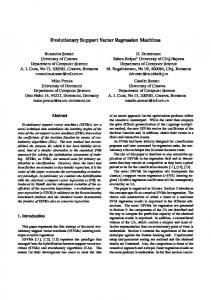
Data Collection Study Area Our 2,601 ha study site (5.1 km ⫻ 5.1 km) is located approximately 10 km southwest of Campbell River on Vancouver Island, British Columbia, Canada (49°52⬘N, 125°20⬘W), where it is composed predominantly of conifer and deciduous forests (Figure 1). Conifer species cover 65 percent of the site and are dominated by approximately 80

(2)

where the parameter C determines the tradeoff between the tolerated training error and the model complexity. ji and j*i are slack variables, which measure the deviation of each training sample point outside the ␧-insensitive zone. These sample points are called support vectors, which will be used to develop regression models. By using a Lagrange function to solve the optimization problem represented in Equation 2, the linear model (Equation 1) can be reformulated as follows: nsv

#

nsv

f (x) ⫽ a (␣i ⫺ ␣*i )8␸(xi) ␸(x)9 ⫹ b ⫽ a (␣i ⫺ ␣*i )K(xi,x) ⫹ b (3) i⫽1

i⫽1

where a*i and ␣i are Lagrange multipliers, which are determined by solving the Lagrange dual problem; and nsv is the number of support vectors. As previously mentioned, only support vectors are used in modeling. The main reason is that the Lagrange multipliers have to be zero for other sample points, where ƒ yi ⫺ f (xi) ƒ 6 ␧. Furthermore, 734

July 2011

Figure 1. (a) Study area located southwest of Campbell River, Vancouver Island, Canada, (b) Lidar canopy height segmentation image (CHS), and (c) QuickBird grayscale image derived from a false color composite using near infrared (NIR), red and green bands.

PHOTOGRAMMETRIC ENGINEERING & REMOTE SENSING

percent Douglas-fir [Pseudotsuga menziesii (Mirb.) Franco], along with small proportions of Western Red Cedar [Thuja plicata (Donn.)], and Western Hemlock [Tsuga heterophylla (Raf.) Sarg.] (Morgenstern et al., 2004). Another 16 percent of the study area is dominated by the deciduous species Red Alder (Alnus rubra Bong.) with the remainder of the site composed of clearcuts, roads and a river that diagonally bisects the site from southeast to northwest. Field Data A number of field stands were visited and twelve plots were chosen to represent various species composition and growing status. Tree information in each plot was measured using a fixed sampling size of 20 m ⫻ 20 m. The center point of each plot was located with differentially corrected GPS (⫹/⫺2 m). All trees with a DBH of more than 10 cm were measured in each plot to obtain mean height, mean DBH, stem density, and species composition. Field-measured AGB and timber volume are typically calculated using field measurements (e.g., DBH, tree height and species composition) and allometric equations. For our purposes, we used Equation 5, as it is widely used in biomass studies in Canada (Lim et al., 2003): AGB ⫽ a1DBHa2

(5)

where a1 and a2 are coefficients. Accurate coefficient values based on species and size were determined from the literature (Ter-Mikaelian and Korzukhin, 1997; Ung et al., 2008). Timber volume was calculated using the Interactive Tree Volume Compiler Software System (TREEVOL), provided by the Government of British Columbia (MSRM, 2009). Lidar Data Lidar data were acquired on 08 June 2004, by an airborne Terrain Scanning Lidar system (Terra Remote Sensing, Inc.; Sidney, Canada). As a discrete return lidar system (Lightwave Model 110), it has a pulse repetition frequency of 10 KHZ, a wavelength of 1,047 nm, a swath width of 56° and a beam divergence of 3.5 mrad. A continuous scanning mode in the typical zigzag pattern was used during data acquisition with a point density of 0.7 points/m2 and a footprint of 0.19 m at nadir. A forest canopy height model (CHM) was generated on a 1.0 m grid with an average height of 19.3 m, and a standard deviation of 8.0 m over the entire forest site. Rather than evaluating individual height pixels, a canopy height segmentation image (CHS) was generated from the CHM to describe forests at the individual tree crown/small tree cluster level (hereafter, tree/cluster level). By adopting this method from Chen and Hay (2011), tree tops were first located with (inverted) crown areas then defined using a watershed algorithm and filled with the average height values from within each crown extent. A height threshold of 2.0 m was used to remove non-tree areas (e.g., tree gaps or shrubs). Qualitative inspection indicated that the watershed objects accurately modeled individual crowns and/or small tree clusters. The average height value was used to fill each segmented tree/cluster, as previous studies show strong correlations within the biophysical parameters we seek (Lefsky et al., 2002; Lim et al., 2003). Table 1 shows the forest proportion of each lidar-measured canopy height class in the study area for three tree classes: (a) all trees, (b) conifers, and (c) deciduous. Height classes were adopted from the British Columbia forest inventory height classes (MFR, 2010). QuickBird (QB) Data A cloud-free QB image was acquired on 11 August 2004 covering the same area as the lidar acquisition. Four multiPHOTOGRAMMETRIC ENGINEERING & REMOTE SENSING

TABLE 1.

PROPORTION OF EACH CANOPY HEIGHT CLASS IN THE STUDY AREA DERIVED FROM THE LIDAR CHS IMAGE Forest Proportion (%)

Canopy Height Class (m) 1: 2: 3: 4: 5:

2.0 10.5 19.5 28.5 37.5

to to to to to

10.4 19.4 28.4 37.4 46.4

All trees

Conifers

Deciduous Trees

7.41 25.11 56.47 10.94 0.07

3.20 19.99 45.60 9.75 0.06

4.21 5.12 10.87 1.19 0.01

spectral bands [i.e., blue, green, red and near infrared (NIR)] and one panchromatic band were used in this study. A principal components spectral sharpening technique (Welch and Ahlers, 1987) was used to combine the spectral information from the QB multispectral bands and the spatial information from the QB panchromatic band, as this method maintains the integrity of the original DNs. The pan-sharpened QB image was then resampled to the same spatial resolution as the CHS (1.0 m). The lidar and pan-sharpened optical data were geometrically co-registered using 118 tie points. A second-order polynomial warping method and nearest neighbor resampling were applied, yielding a RMSE of 0.85 m. Due to the dense forest cover in this area, co-registration was performed using tree tops only.

Data Analysis imagery were first segmented using a GEOBIA approach to produce image-objects at an average size representing the small tree cluster level (0.04 ha). Transect-covered imageobjects were then used as training samples to extract variables from corresponding locations in both QB and lidar data. By using these variables, multiple regression and SVR models were developed to estimate lidar-measured canopy height for the entire study area. The estimated canopy heights from both types of models were evaluated against the full-scene lidar dataset. This was followed by the prediction of field-measured canopy height, AGB and volume using field measurements. The flowchart in Figure 2 QB

Figure 2. Flowchart of the research process with reference to Data Analysis sections.

July 2011

735

summarizes these steps; while the following sub-sections provide greater detail and explanation. Image Segmentation High spatial resolution, optical remotely sensed data can meet the increasing need to characterize forest ecosystems at fine spatial scales (Wulder et al., 2004a). However, in our case, individual pixels represent only a small portion of the forest objects (e.g., individual trees or tree clusters) of interest. To acquire additional landscape details while reducing the spectral variability within each object, GEOBIA provides an advantageous alternative to the traditional pixel-based approach by using image-objects (i.e., groups of connected pixels that are relatively homogeneous and different from their surroundings) as the basic study units (Hay and Castilla, 2008; Blaschke, 2010). Unlike pixels, where size and (square) shape have been limited by specific sensors, image-objects exhibit various object size and shape. In the case of forest studies, object size facilitates research on individual trees, small tree clusters or large forest stands, etc. In addition, object’s boundaries provide a tailored window shape, or filter from which to extract image-texture information (Hay et al., 1996). Since part of our objective is to estimate forest biophysical parameters at the object-level, our objects of interest were automatically generated by applying the image segmentation software: Size-Constrained Region Merging (SCRM) (Castilla et al., 2008) to the pan-sharpened multispectral QB dataset. SCRM has two advantages over currently existing segmentation algorithms: (a) the object size (e.g., mean, minimum and maximum) can easily and explicitly be controlled through input parameters; and (b) the defined object shapes (composed of smooth boundaries) are similar to those delineated by experienced forest analysts. It should be noted that large mean object sizes (MOS) tend to ignore the forest height variability within individual objects, as numerous smaller units are merged into fewer larger units (Chen et al., 2010). To better capture forest variability and to benefit from the high-resolution characteristics of the optical and lidar data (i.e., height, image texture, and shadow), we selected a relatively small MOS of 0.04 ha; which is similar to the size of our field plots. Extraction of Variables Previous studies have shown that relationships exist between optical bands and forest height (Franklin and

McDermid, 1993; Hyde et al., 2006; Donoghue and Watt, 2006; Chen et al., 2010). In order to extend canopy height information from the small area(s) covered by lidar transects to the entire study area, the QB scene was used to extract three types of independent variables as outlined in Chen et al. (2010): (a) spectral, (b) image-texture, and (c) shadow variables. Specifically, (a) the mean DN within each imageobject was calculated for each spectral band: blue, green, red and NIR; (b) Two styles of image-texture measures were considered: internal-object texture )a measure of the spatial variability of DNs within an image-object) and geographic object-based texture (GEOTEX) (a measure of the spatial variability within neighboring objects); and (c) Shadow fraction, a quotient of the size of shaded areas and the size of the corresponding forest objects, was then calculated based on the DNs of the NIR band. The CHS was used to extract the dependent variable of canopy height, which is the average height within the same image-objects as those derived from QB segmentation. Image-objects covered by transects were used as training samples to develop robust regression and SVR models (as described in the following two Sections). Four types of lidar transect areas, 8.8 percent (one transect), 17.6 percent (two transects), 26.4 percent (three transects) and 35.2 percent (four transects) and their locations, were extracted and compared in this study (Figure 3). Transect size and location were determined by adopting the lidar transect selection strategies developed by Chen and Hay (in review), which created a canopy pseudo-height image from high-spatial resolution optical data and automatically selected “optimal” lidar transects based on proportionally matching the canopy height structure (i.e., height histogram) of the full scene, with that of the transect(s). Here, “optimal” refers to the least amount of transect samples (thus lower acquisition costs) and most accessible location(s) to meet specific sampling objectives. In this study, specific transects and their locations were chosen for three reasons: (a) transect size was based upon the actual acquired lidar swath width of 450 m, or 8.8 percent of the total study area; (b) Previous results (Chen and Hay, 2011) show that a minimum of four different lidar transect areas represent a sufficient amount of training samples necessary to evaluate the different models. Additionally, we are interested in minimizing lidar acquisition costs; and (c) Based on the selection strategies applied, each transect covers a (proportionally) similar canopy height distribution as that derived from the full lidar scene.

Figure 3. These four types of transects represent the “optimal” selected flight lines that best meet the lidar transect selection strategies for flight line number (1 through 4), their locations, and their area covered (as a percent of total study site): (1) 8.8 percent, (2) 17.6 percent, (3) 26.4 percent, and (4) 35.2 percent (Chen and Hay, 2011). For illustrative purposes, the QB image was used as the base layer with lidar transects overlaid.

736

July 2011


Multiple Regression Model Chen et al. (2010) investigated the potential of using multiple regression to estimate lidar-measured canopy height with QB data. An important finding was that models formulated using a combination of exponential and quadratic form performed better than a simple linear model. Therefore, the same type of nonlinear multiple regression model was employed in this study to relate QB-derived independent variables with the lidar-derived dependent variable: n

CH ⫽ exp( a (aiX2i ⫹ biXi ⫹ ci))

(6)

i⫽0

where CH is the lidar-measured canopy height; Xi is the ith independent variable; ai, bi, and ci are coefficients for the ith variable; and n is the number of independent variables. To better describe different forest types, separate regression models were developed for conifer and deciduous trees. A stepwise variable selection method, used by Wulder et al. (2004b), was adopted in this study to determine the most significant input variables for modeling. Support Vector Regression (SVR) Model As previously described in this paper, the performance of SVR is highly affected by three model parameters: C, ␧, and ␥. Thus, a two-step grid-search technique, recommended by Hsu et al. (2009), was used in this study to select the optimal model parameters. Due to the independence of these parameters, the main idea of this technique is to use a cross-validation method to evaluate all potential parameter combinations; with the best combination producing the highest cross-validation accuracy. In this study, a 10-fold cross-validation technique was applied. To avoid a time-consuming exhaustive search, two steps were performed as follows: (a) the coarse search was conducted using relatively large grid intervals, i.e., C ⫽ [2⫺1, 20, 21, 22, 23], ␧ ⫽ [2⫺7, 2⫺6, 2⫺5, 2⫺3, 2⫺2, 2⫺1, 20] and ␥ ⫽ [2⫺7, 2⫺6, 2⫺5, 2⫺3, 2⫺2, 2⫺1, 20, 21]; and (b) the fine search was conducted using relatively small grid intervals, e.g., [2k⫺0.75, 2k⫺0.50, 2k⫺0.25, 2k, 2k⫹0.25, 2k⫹0.50, 2k⫹0.75], where 2k represents the best calculation parameter from step (a). The parameter ranges were determined from trial-and-error. This style of using exponentially growing sequences has proven effective for finding the best candidate parameters (Hsu et al., 2009). Conifer and deciduous trees were separately modeled using SVR. In this study, the SVM open source software of LIBSVM was used to perform the modeling (Chang and Lin, 2001), with the best parameter combination found at C ⫽ 8, ␧ ⫽ 0.5 and ␥ ⫽ 1 for both tree species. It should be noted that SVR used the same input variables as those selected for multiple regression through the stepwise variable selection. This allows these two types of models to be compared in a straightforward way. Comparison of Model Performance for Estimating Lidar-measured Canopy Height Multiple regression and SVR models were developed using the training samples within the lidar transect-covered area(s). The variables extracted from the full QB scene were then imported into both models to estimate (lidar-measured) canopy height for the entire study site. Results were evaluated by comparing the estimated canopy height with the full lidar scene (i.e., CHS), and the RMSE (root mean square error) was reported. Specifically, the comparison of model performance was made for four types of transect extents, and two tree types (i.e., conifer and deciduous). PHOTOGRAMMETRIC ENGINEERING & REMOTE SENSING

Estimation of Field-measured Canopy Height, Above-ground Biomass (AGB) and Volume Nonlinear models with a natural logarithm form were developed to build a relationship between the previously estimated canopy height and their corresponding field measurements: Mf ⫽ b 0hbE 1

(7)

where Mf is the field measurement (e.g., canopy height, AGB or volume), hE is the estimated canopy height; and ␤0 and ␤1 are coefficients. This formula has been used to successfully estimate forest biophysical parameters directly from lidar data in several studies (Næsset, 1997; Means et al., 1999; Lim et al., 2003). Since it is not practical to build two models for two tree species using just twelve field plots, only one model was developed for estimating each forest biophysical parameter without distinguishing conifers and deciduous trees. A leave-one-out cross-validation technique was chosen to evaluate model performance using RMSE.

Results and Discussion Comparison between four types of transect extents Different errors for estimating lidar-measured canopy height using four types of lidar transect extents and locations are illustrated in Figure 4. Larger transect extents represent more training data, which typically facilitates a higher accuracy estimation. This was illustrated by both models using multiple regression and SVR. For multiple regression, the error for all trees dropped from 7.9 m to 7.0 m with an increase of transect extent from 8.8 percent to 35.2 percent, while the error decreased from 6.2 m to 5.6 m using SVR. Though a low error of 6.2 m was achieved with multiple regression using two lidar transects (i.e., 17.6 percent), models using SVR performed better at defining all trees than those using multiple regression for each different transect type. For example, when only a single lidar transect was selected for modeling, the canopy height estimation performance increased by 21.5 percent (from 7.9 m to 6.2 m) using SVR versus multiple regression. This also confirms the argument that SVR has a strong generalization capacity even

Figure 4. Comparison of full scene canopy height estimation errors for all trees using four different lidar transect extents: one flight line (8.8 percent), two flight lines (17.6 percent), three flight lines (26.4 percent), and four flight lines (35.2 percent).

July 2011

737

Figure 5. Comparison of the canopy height estimation errors for all trees, defined in five height classes extracted from four lidar transect extents (see Figure 3): (a) 8.8 percent, (b) 17.6 percent, (c) 26.4 percent and (d) 35.2 percent. The five height classes are: HTC1 (2.0 to 10.4 m), HTC2 (10.5 to 19.4 m), HTC3 (19.5 to 28.4 m), HTC4 (28.5 to 37.4 m), and HTC5 (37.5 to 46.4 m), which are similar to the British Columbia forest inventory height classes.

when using a small number of training samples (Cristianini and Shawe-Taylor, 2000). Figure 5 further presents the errors of estimating lidarmeasured canopy height for five canopy height classes using four transect extents. The height classes were adopted from the British Columbia forest inventory height classes (MFR, 2010), except our base-height started from 2.0 m instead of the original 0.0 m, so as to remove low-elevation shrubs and bushes. A similar error trend as that shown in Figure 4 was also found in Figure 5. Specifically, for both models, low errors were located in height classes 2 (10.5 to 19.4 m) and 3 (19.5 to 28.4 m). The main reason was that these two classes represented a proportionally large sample (i.e., 81.58 percent) of all height classes in the entire study area (Table 1). This also explains why the errors increased for other classes, especially for height class 5 (37.5 to 46.4 m), which proportionally accounted for only 0.07 percent (i.e., 1.5 ha) of the full site. As a result, the corresponding canopy height error was larger than 15 m (Table 1 and Figure 5). This strongly suggests that the performance of both types of models is biased to the proportionally largest height classes. Additionally, Figure 5 shows that SVR models were more adaptive to estimate canopy heights above 19.5 m (i.e., height classes 3, 4, and 5); while multiple regression models were better at predicting lower canopies (i.e., height classes 1 and 2) using a combination of exponential and quadratic form. However, it should be noted, for height class 3 (with the largest forest proportion of 56.47 percent), the average error decreased by 33.3 percent (from 6.6 m to 4.4 m) using SVR compared with multiple regression.

difficult to accurately estimate their canopy height (Figure 6). As a result, all models developed for conifers (for all transect types), performed better than those developed for deciduous trees. Specifically, the average errors decreased by 20.3 percent (from 7.9 m to 6.2 m) for multiple regression, and 20.4 percent (from 6.9 m to 5.5 m) for SVR. Figure 6 further shows that SVR models achieved better results than multiple regression for both tree types, except in the case of the 17 percent lidar cover, where deciduous multiple regression was slightly better. In addition, the SVR-estimated deciduous canopy height error reached similar accuracies as those of conifers using multiple regression; again, with the exception of the 17.6 percent lidar cover. Similar to Figure 5, both conifer and deciduous trees had relatively better estimation results when the corresponding canopy height classes accounted for a larger proportion of the forested site (Figure 7 and Table 1). In the case of a single lidar transect, the best height estimate for conifers was 4.2 m derived from a SVR model at height class 3; while the best estimate for deciduous trees was 5.7 m derived from a SVR model at the height class 2. Initially, we did not expect that at height class 1 (2.0 to 10.4 m) the small deciduous trees would achieve better results than small conifers. However, when we re-evaluated the optical and lidar data based on these findings, we could see that the tight structural crown composition of these smaller trees was much simpler than the overlapping complex crowns of the taller deciduous classes; where, the spectral reflectance of small conifers tend to be heavily influenced by tree gaps.

Comparison between Conifers and Deciduous Trees Compared to conical-shaped conifers, deciduous canopies typically exhibit complex irregular shapes, making it more

Comparison between Model Estimates and Field Measurements Reduced lidar cover represents lower lidar data acquisition and processing costs. However, it should be noted that

738

July 2011


Figure 6. Comparison of full scene canopy height estimation errors for conifers and deciduous trees from four different lidar transect extents, shown as a percent of the total area.

Figure 8 illustrates the scatterplots of field measurements versus estimates of canopy height, AGB, and volume; with canopy height producing the best result (R2: 0.81; RMSE: 4.0 m). The coefficient of determination for estimating AGB and volume were 0.76 and 0.64, with errors of 63.1 Mg/ha and 156.9 m3/ha, respectively. We expected better performance for estimating canopy height, as the height values were acquired from field measurements. Field AGB and volume were calculated using allometric equations, where parameter errors may have been introduced. Compared to previous studies that have combined lidar transects and optical data to estimate canopy height, our height estimation error is slighter larger, e.g., 4.0 m versus 3.2 m in Wulder and Seemann (2003) and 3.5 m in Hilker et al. (2008). However, it should be noted that our results were derived at the small plot level; whereas, these two studies were conducted at a larger stand level.

Conclusions (depending on the sampling scheme), this may also lower the model accuracy due to fewer training samples. Therefore, the best decision needs to be made based on the actual project requirements. In this case, we noticed that in most conditions, SVR models produced better results than multiple regression models. Additionally, by using SVR, the errors for estimating lidar-measured canopy height varied stably using different optimal transects. For example, the standard deviation of height error derived from all lidar transects (i.e., 6.2 m, 5.9 m, 5.7 m, and 5.6 m) is only 0.2 m (Figure 4). Therefore, the canopy height estimation results derived from SVR using a single lidar transect (i.e., 8.8 percent extent) was chosen as the best when considering both cost and accuracy. As a result, these data were used to generate the following canopy height, AGB, and volume, simulating field measurements.

In this study, we have introduced SVR, a machine learning technique, to estimate the forest biophysical parameters of canopy height, AGB, and volume for a full study area (2,601 ha), by combining high-resolution (1.0 m) QuickBird imagery and lidar transects, that represent 8.8 percent, 17.6 percent, 26.4 percent and 35.2 percent of the total site area. We have also applied a GEOBIA approach to generate all estimates at a small tree cluster level, i.e., MOS (mean object size) of 0.04 ha. Based on a comparison with multiple regression models, the following conclusions can be drawn: • For both conifers and deciduous trees, SVR models resulted in better performance in all conditions, except for the case of 17 percent lidar cover, where deciduous trees were better modeled by multiple regression. Although deciduous trees typically have more complex canopy structures than conifers and are thus more difficult to model, the use of SVR dramatically improved

Figure 7. A comparison of the full scene canopy height estimation errors for conifers versus deciduous, generated from four different types of transects (see Figure 3): (a) 8.8 percent, (b) 17.6 percent, (c) 26.4 percent, and (d) 35.2 percent. Five height classes are: HTC1 (2.0 to 10.4 m), HTC2 (10.5 to 19.4 m), HTC3 (19.5 to 28.4 m), HTC4 (28.5 to 37.4 m), and HTC5 (37.5 to 46.4 m), which are similar to the British Columbia forest inventory height classes.


July 2011

739

Figure 8. Field measurements versus estimates for (a) canopy height, (b) AGB, and (c) volume, based on an “optimal” single lidar transect representing 8.8 percent of the total site area.

the height estimation performance for deciduous trees. In several cases, deciduous results showed similar accuracy to those of conifers using multiple regression. • For different canopy height classes, both models showed better results for the classes that proportionally accounted for larger areas (i.e., samples). This may be explained by the selection of lidar transects which were based on rules to match the height variability of the entire study site; which in this case was biased to specific species and height classes. • SVR provided better results for height classes that when combined, represented more than 80 percent of the entire forested area. This suggests that the transect selection method used (Chen and Hay, 2011) could be enhanced by including a new rule to account for class proportionality. This would also allow a user to specify (i.e., bias) the selection of one or more specific height classes of interest. For example, logging activities may be of interest in high AGB and/or volume stands that only account for a small proportion of the landscape-level inventory, i.e., old growth or seed stock. • The SVR model errors revealed a more stable trend using different transect extents. This supports the argument that SVR has a strong generalization capacity using a small number of training samples (Cristianini and Shawe-Taylor, 2000). By using the canopy height estimated from a single lidar transect and SVR, a strong relationship was found between predicted and field-measured canopy height (R2: 0.81; RMSE: 4.0 m). However, AGB (R2: 0.76; RMSE: 63.1 Mg/ha) and volume (R2: 0.64; RMSE: 156.9 m3/ha) were more difficult to predict. One possible reason could be that the AGB and volume field data contained errors introduced by the allometric equation parameters. Additionally, more

740

July 2011

detailed species information may be needed for estimating these two parameters. • In order to model canopy height variability at a fine scale, this research was performed at the tree crown/cluster level using a mean object size of 0.04 ha. In future studies, we will investigate the potential of using this SVR approach for forest inventory update at an object stand-level of 1.0 ha and greater.

Acknowledgments This research has been supported by an Alberta Informatics Circle of Research Excellence (ICORE) Ph.D. scholarship awarded to Gang Chen. We appreciate the generous use of QuickBird and lidar data provided by Dr. Benoît St-Onge at the University of Quebec at Montreal and the insightful comments from three anonymous reviewers.

References Blaschke, T., 2010. Object based image analysis for remote sensing, ISPRS Journal of Photogrammetry and Remote Sensing, 65(1):2–16. Castilla, G., G.J. Hay, and J.R. Ruiz, 2008. Size-constrained region merging (SCRM): An automated delineation tool for assisted photointerpretation, Photogrammetric Engineering and Remote Sensing, 74(4):409–419. Chang, C.-C., and C.-J. Lin, 2001. LIBSVM: A Library for Support Vector Machines, URL: http://www.csie.ntu.edu.tw/⬃cjlin/libsvm (last date accessed: 10 April 2011). Chen, G., G.J. Hay, G. Castilla, B. St-Onge, and R. Powers, 2010. A multiscale geographic object-based image analysis (GEOBIA) to


estimate lidar-measured forest canopy height using QuickBird imagery, International Journal of Geographical Information Science, in press. Chen, G., and G.J. Hay, 2011. An airborne lidar sampling strategy to model forest canopy height from QuickBird imagery and GEOBIA, Remote Sensing of Environment, 115(6):1532–1542. Cristianini, N., and J. Shawe-Taylor, 2000. An Introduction to Support Vector Machines and Other Kernel-Based Learning Methods, Cambridge, U.K., Cambridge University Press, 2000, 189 p. Dong, J., R.K. Kaufmann, R.B. Myneni, C.J. Tucker, P.E. Kauppi, J. Liski, W. Buermann, V. Alexeyev, and M.K. Hughes, 2003. Remote sensing estimates of boreal and temperate forest woody biomass: Carbon pools, sources, and sinks, Remote Sensing of Environment, 84(3):393–410. Donoghue, D.N.M., and P.J. Watt, 2006. Using LiDAR to compare forest height estimates from IKONOS and Landsat ETM⫹ data in Sitka spruce plantation forests, International Journal of Remote Sensing, 27(11):2161–2175. Franklin, S.E., and G.J. McDermid, 1993. Empirical relations between digital SPOT HRV and CASI spectral response and lodgepole pine (Pinus contorta) forest stand parameters, International Journal of Remote Sensing, 14(12):2331–2348. Gunn, S.R., 1998. Support Vector Machines for Classification and Regression, Technical Report, 66 p. Hay, G.J., and G. Castilla, 2008. Geographic Object-Based Image Analysis (GEOBIA). Object-Based Image Analysis - Spatial Concepts for Knowledge-driven Remote Sensing Applications (T. Blaschke, S. Lang, and G.J. Hay, editors), Berlin, SpringerVerlag, pp. 75–89. Hay, G.J., K.O. Niemann, and G.F. McLean, 1996. An object-specific image-texture analysis of H-resolution forest imagery, Remote Sensing of Environment, 55(2):108–122. Hese, S., W. Lucht, C. Schmullius, M. Barnsley, R. Dubayah, D. Knorr, K. Neumann, T. Riedel, and K. Schroter, 2005. Global biomass mapping for an improved understanding of the CO2 balance-The Earth observation mission Carbon-3D, Remote Sensing of Environment, 94(1):94–104. Hilker, T., M.A. Wulder, and N.C. Coops, 2008. Update of forest inventory data with lidar and high spatial resolution satellite imagery, Canadian Journal of Remote Sensing, 34(1):5–12. Hsu, C.-W., C.-C. Chang, and C.-J. Lin, 2009. A Practical Guide to Support Vector Classification, Technical Report, 15 p. Huang, C., K. Song, S. Kim, J. Townshend, P. Davis, J. Masek, and S.N. Goward, 2008. Use of a Dark Object Concept and Support Vector Machines to automate forest cover change analysis, Remote Sensing of Environment, 112(3):970–985. Hudak, A.T., M.A. Lefsky, W.B. Cohen, and M. Berterreche, 2002. Integration of LIDAR and Landsat ETM⫹ data for estimating and mapping forest canopy height, Remote Sensing of Environment, 82(2–3):397–416. Hyde, P., P. Dubayah, W. Walker, J.B. Blair, M. Hofton, and C. Hunsaker, 2006. Mapping forest structure for wildlife habitat analysis using multi-sensor (LiDAR, SAR/InSAR, ETM⫹, QuickBird) synergy, Remote Sensing of Environment, 102(1–2):63–73. Kuemmerle, T., O. Chaskovskyy, J. Knorn, V.C. Radeloff, I. Kruhlov, W.S. Keeton, and P. Hostert, 2009. Forest cover change and illegal logging in the Ukrainian Carpathians in the transition period from 1988 to 2007, Remote Sensing of Environment, 113(6):1194–1207.


Lefsky, M.A., W.B. Cohen, D.J. Harding, G.G. Parkers, S.A. Acker, and S.T. Gower, 2002. Lidar remote sensing of above-ground biomass in three biomes, Global Ecology & Biogeography, 11(5):393–399. Lim, K., P. Treitz, K. Baldwin, I. Morrison, and J. Green, 2003. Lidar remote sensing of biophysical properties of tolerant northern hardwood forests, Canadian Journal of Remote Sensing, 29(5):658–678. Means, J.E., S.A. Acker, D.J. Harding, J.B. Blair, M.A. Lefsky, W.B. Cohen, M.E. Harmon, and W.A. McKee, 1999. Use of largefootprint scanning airborne lidar to estimate forest stand characteristics in the Western Cascades of Oregon, Remote Sensing of Environment, 67(3):298–308. MFR (Ministry of Forests and Range), the British Columbia Government, Canada, 2010. URL: https://psc2.for.gov.bc.ca/ RESULTS/HELP/Results_Online_Help/Pop_ups/pop_Height_ Class.htm. Morgenstern, K., T.A. Black, E.R. Humphreys, T.J. Griffis, G.B. Drewitt, T.B. Cai, Z. Nesic, D.L. Spittlehouse, and N.J. Livingstone, 2004. Sensitivity and uncertainty of the carbon balance of a Pacific Northwest Douglas-fir forest during an El Nino La Nina cycle, Agricultural and Forest Meteorology, 123(3–4):201–219. MSRM (Ministry of Sustainable Resource Management), the British Columbia Government, Canada, 2010. Interactive Tree Volume Compiler Software System (TREEVOL), Version: 2.12.21. Næsset, E., 1997. Estimating timber volume of forest stands using airborne laser scanner data, Remote Sensing of Environment, 61(2):246–253. Natural Resources Canada, 2009. The State of Canada’s Forests Annual Report 2009, Canadian Forest Service, Natural Resources Canada, Ottawa, 64 p. Smola, A.J., and B. Schölkopf, 2004. A tutorial on Support Vector Regression, Statistics and Computing, 14(3):199–222. Ter-Mikaelian, M.T., and M.D. Korzukhin, 1997. Biomass equations for sixty-five North American tree species, Forest Ecology and Management, 97(1):1–24. Ung, C.-H., P.Y. Bernier, and X. Guo, 2008. Canadian national biomass equations: New parameter estimates that include British Columbia data, Canadian Journal of Forest Research, 38(5):1123–1132. Vapnik, V., 1995. The Nature of Statistical Learning Theory, New York, Springer-Verlag, 188 p. Vapnik, V., 1998. Statistical Learning Theory, New York, Wiley, 736p. Welch, R., and W. Ahlers, 1987. Merging multiresolution SPOT HRV and Landsat TM data, Photogrammetric Engineering & Remote Sensing, 53(3):301–303. Wulder, M.A., R.J. Hall, and N.C. Coops, 2004a. High spatial resolution remotely sensed data for ecosystem characterization, Bioscience, 54(6):511–521. Wulder, M.A., R. Skakun, W. Kurz, and J. White, 2004b. Estimating time since forest disturbance using segmented Landsat ETM⫹ imagery, Remote Sensing of Environment, 93(1–2):179–187. Wulder, M.A., and D. Seemann, 2003. Forest inventory height update through the integration of LIDAR data with segmented Landsat imagery, Canadian Journal of Remote Sensing, 29(5):536–543. (Received 15 September 2010; accepted 22 December 2010; final version 03 February 2011)

July 2011

741