A System Dynamics Software Process Simulator for Staffing Policies Decision Support Dr. James Collofello Dept. of Computer Science and Engineering Arizona State University Tempe, Arizona 85287-5406 (602) 965-3190
[email protected] Ioana Rus, Anamika Chauhan Dept. of Computer Science and Engineering Arizona State University
Dan Houston Honeywell, Inc. and Dept. of Industrial and Management Systems Engineering Arizona State University Douglas Sycamore Motorola Communication Systems Divsions Scottsdale, Arizona Dr. Dwight Smith-Daniels Department of Management Arizona State University
Abstract Staff attrition is a problem often faced by software development organizations. How can a manager plan for the risk of losses due to attrition? Can policies for this purpose be formulated to address his/her specific organization and project? Proposed was to use a software development process simulator tuned to the specific organization, for running "what-if" scenarios for assessing the effects of managerial staffing decisions on project's budget, schedule and quality. We developed a system dynamics simulator of an incremental software development process and used it for analyzing the effect of the following policies: to replace engineers who leave the project, to overstaff in the beginning of the project or to do nothing, hoping that the project will still be completed in time and within budget. This paper presents the simulator, the experiments that we ran, the results that we obtained and our analysis and conclusions. Introduction We used process modeling and simulation for estimating the effect on the project cost, schedule and rework of different staffing policies. Assessment of such managerial decisions could be also done by other methods like formal experiments, pilot projects, case studies, and experts opinions and surveys. Modeling and simulation is preferred because it does not have the disadvantages of the other methods (like possible irrelevance in the case of formal experiments or pilot projects, interfering with the real process and taking a
long time for case studies or subjectivity for experts opinions and surveys). System Dynamics Modeling A software process model represents the process components (activities, products, and roles), together with their attributes and relationships, in order to satisfy the modeling objective. Some modeling objectives are to facilitate a better human understanding and communication, and to support process improvement, process management, automated guidance in performing the process, and automated process execution [6]. In addition, we demonstrate how process modeling experimentation can be used to investigate alternatives for organizational policy formulation. There are many modeling techniques developed and used so far, according to the modeling goal and perspective. The paradigm chosen for this research was system dynamics modeling. Richmond considers system dynamics as a subset of systems thinking. Systems thinking is "the art and science of making reliable inferences about behavior by developing an increasingly deep understanding of underlying structure" [11]. Systems thinking is, according to Richmond, a paradigm and a learning method. System dynamics is defined as "the application of feedback control systems principles and techniques to modeling, analyzing, and understanding the dynamic behavior of complex systems" [2]. System dynamics modeling (SDM) was developed in the late 1950's at M.I.T. SDM is based on cause-effect relationships that are observable in a real system. These cause-effect relationships constantly interact while the computer model is being executed, thus the dynamic
interactions of the system are being modeled, hence its name. A system dynamics model can contain relationships between people, product, and process in a software development organization. The most powerful feature of system dynamics modeling is realized when multiple cause-effect relationships are connected forming a circular relationship, known as a feedback loop. The concept of a feedback loop reveals that any actor in a system will eventually be affected by its own action. Because system dynamics models incorporate the ways in which people, product, and process react to various situations, the models must be tuned to the organizational environment that they are modeling. SDM is a structural approach, as opposed to other estimation models like COCOMO and SLIM, that are based on correlation between metrics from a large number of projects. The automated support for developing and executing SDM simulators enables handling the large complexity of a software development process which can not be handled by a human mental model. Building and using the model results in a better understanding of the cause-effect relationships that underlie the development of software. A simulator to be used for estimating, predicting, and tracking a project requires a quantitative modeling technique. SDM utilizes continuous simulation through evaluation of difference and differential equations. These equations implement both the feedback loops that model the project structures as flows, as well as the rates that model the dynamics of these flows. Thus, application of an SDM model requires an organization to define its software development processes and to identify and collect metrics that characterize these processes. Simulation enables experimenting with the model of the software process, without impacting on the real process. The effects of one factor in isolation can be examined, which cannot be done in a real project. The outcome of the SD simulation has two aspects: an intellectual one, consisting of a better understanding of the process and a practical one, consisting of prediction, tracking, and training. SDM was applied to the software development process for the first time by Tarek Abdel-Hamid and Stuart Madnick [2]. Their model captures the managerial aspects of a waterfall software life cycle. It was the starting point for many subsequent models of the entire process [15], [14] or parts of it [5] and [9] that have been successfully used for resource management [8], [13], process reengineering [4], project planning, and training [12]. Abdel-Hamid [1] studied the impact of turnover, acquisition, and assimilation rates on software project cost and schedule. He found that these two response variables can be significantly affected by an
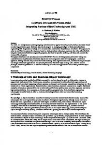
employment time of less than 1000 days, by a hiring delay less than or greater than 40 days, or by an assimilation delay greater than 20 days. We take this discussion a step further into the practical realm by focusing on the turnover issue and demonstrate how SDM can be used in decision support for strategies that address staff turnover. Description of System Dynamics Model Our system dynamics modeling tool was developed using the ithink simulation software [7]. The model incorporates four basic feedback loops comprised of non-linear system dynamic equations. The four feedback loops were chosen because they encompass the factors that are typically the most influential in software projects [16]. All of these feedback loops begin and end at the object labeled, Schedule and Effort, which is the nucleus of the system. This object represents a project schedule and the effort in person hours to complete a schedule plan. See Figure 1. The first feedback loop represents the staffing profile of a project (refer to the loop “Schedule and Effort”, “Staffing Profile”, “Experience Level”, and “Productivity” on Figure 1). The staffing profile affects productivity based on the number of engineers working on a project, the domain expertise of the engineers, and amount of time an engineer participates on a project. The second feedback loop models the communication overhead (refer to the loop “Schedule and Effort”, “Staffing Profile”, “Communication Overhead”, and “Productivity” on Figure 1). The more people on a project will result in an increase in communication overhead among the team members and thus, decreases the productivity efficiency [14] [15]. The third feedback loop takes into consideration the amount of defects generated by the engineers during the design and coding phases of an increment, which translates into rework hours (refer to the loop “Schedule and Effort”, “Staffing Profile”, “Experience Level”, “Defect Generated, and “Rework Hours” on Figure 1). The tool also models the impact of domain expertise on defect generation. An engineer with less domain expertise generates more defects than an engineer with a higher degree of domain expertise. The fourth feedback loop models the schedule pressure associated with the percentage of work complete per the schedule (refer to the loop “Schedule and Effort”, “Schedule Pressure”, and “Productivity” on Figure 1). The farther behind schedule the greater the schedule pressure. As schedule pressure increases, engineers will work more efficiently and additional hours, increasing productivity toward completing the work. However, if schedule pressure remains high and
engineers are working many hours of overtime, they begin to generate more defects and eventually an exhaustion limit is reached. Once the exhaustion
limit is reached, productivity will decrease until a time period such that the engineers can recoup and begin working more productively again.
Schedule Pressure
Schedule and Effort
Rework Hours
Productivity Defects Generated
Staffing Profile Communication Overhead Experience Level
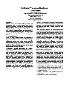
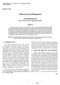
Figure 1. Basic Feedback Loops of the Model The model inputs are summarized in Table 2 familiar. For a summary of the experts’ credentials, The model outputs are provided in the form of refer to Table 1. graphs that plot the work remaining in each Each expert (or evaluator) was asked to review the increment, current staff loading, total cost, percent tool from a Project Leader position, a Software complete, and quality costs. Figure 2 is an example Developer position, and to assess the tool's technical of the output that shows the graph for Staff Loading characteristics. During the simulations, the experts and Total Cost plots. were to observe the output for valid trend data and for The model was validated by two methods, expert a level of comfort with the accuracy of the results. opinion and reproduction of actual project results. Six The demo given to each expert was identical. After experts from Motorola and very experienced software completing the demo, the experts were given an professionals, examined the simulator model and opportunity to run different scenarios with the expressed their confidence in its ability to model the supplied data or scenarios with their own project data. general behavior of a software project. In addition, Finally, they were given an opportunity to compare one of the experts used the model to accurately the results to any project manage tools they use. reproduce the results of a project with which he was
Table 1. Background Summary of Each Expert Expert #1
Expert #2
Expert #3
Expert #4
Expert #5
Expert #6
Title: Principal Software Engineer Degrees: M.S. and Ph.D. in Computer Science Years of Experience: 13 Years Responsibilities: Project Leader, Systems Engineer, Software Engineer, and Proposal Development. Other Pertinent Information: Former Assistant Professor of Computer Science at Arizona State University, Tempe, AZ. Title: Principal Software Engineer Degrees: Ph.D. in Computer Science Years of Experience: 25+ Years Responsibilities: Project Leader Other Pertinent Information: Former Assistant Professor of Computer Science at Arizona State University, Tempe, AZ. Title: Software Engineer Degrees: B.S in Computer Science Years of Experience: 11 years Responsibilities: Software Development - Currently developing a ManMachine Interface. Special Awards: Special Achievement Award, 1987 - Naval Avionics Center Exceptional Performance, 1991 - Motorola GSTG, CSO Engineering Award, 1993 - Motorola GSTG Title: Software Engineer Degrees: M.S. in Computer Science; M.B.A. in Management Years of Experience: 33 Years Responsibilities: Developing software for a medium size aerospace project. Other Pertinent Information: A retired Air Force Lieutenant Colonel. Title: Chief Software Engineer Degrees: B.S. in Electrical Engineering Years of Experience: 39 Years Responsibilities: Software Process and Quality Special Awards: Dan Nobel Fellow Award (Motorola); IEEE contributor Other Pertinent Information: Author: Motorola GED's Software Process Manual. Instructor: Motorola GED Project Leader Training. Chair: Motorola GED Software Metrics Working Group. Chair: Motorola GED Software Training Program Working Group. Member: Motorola GED Software Defect Prevention Working Group. Three Patents. Developing software fault occurrence and prediction model. Title: Engineering Metrics Manager Degrees: B.S. in Electrical Engineering Years of Experience: 35 Years Responsibilities: Coordinate collection and analysis of Engineering metrics.
Overall, the tool fared extremely well against the evaluation process and the experts were quite pleased with the results. There were two particularly exciting highlights that occurred during the reviews with expert #3 and expert #5 that are worth noting.
The first highlight was seeing the results from simulating expert #3's Man-Machine Interface project, which was 80% completed. Before simulating the project, some actual historical data along with some remaining estimated data to complete the ManMachine Interface project was entered into the simulator. After simulating the project with actual
and estimated data, Currently the simulator tracked there is an updated Number of increments 3 within a couple of version of the Productivity percentage points of simulator tool that Engineer 1 (domain inexperienced) .8 expert #3's actual and has been Engineer 2 (domain experienced) 1.0 predicted results. incorporated into a Engineer 3 (very domain 1.2 The second corporate training experienced) highlight was program. The Defect generation rates simulating three sets simulator is being Engineer 1 (domain inexperienced) .0300/hr of project data used to Engineer 2 (domain experienced) .0250/hr supplied by expert #5. demonstrate an Engineer 3 (very domain .0225/hr He generated these incremental experienced) three scenarios with development Defect detection the aid of the approach over a % of defects found in peer reviews 80% COCOMO tool for waterfall % of defects found in integration test 20% the three engineering development Percent of schedule allocated to rework 10% activities: Detail approach, peer Defect removal costs Design, Code and review Found in peer reviews 2 hr/defect Unit Test, and effectiveness, Found in integration testing 10 hr/defect Integration. After schedule simulating the three compression scenarios, expert #5 concurred that the simulator concept, mythical man-month perception, and the produced believable results for all three scenarios [14]. 90% completion syndrome. Description of the experiment Attrition is clearly detrimental to a software development project. When an experienced developer leaves a project prior to its completion, then a project manager faces the question of whether to replace the departing individual or to forego the expense of replacement and make other adjustments, such dropping functionality, slipping the schedule, and rearranging assignments. The answer to the question of replacement may turn on factors such as the experience of the developer, the percent completion of the project, the number of engineers on the project, the
time required for hiring or transfer, and the attrition rate of the organization. Replacement is costly, but may be required to keep a project on schedule. It leads one to wonder, can the dilemma presented by attrition be resolved by yet another alternative, that of staffing a project with more than the necessary number of development engineers? Are there project situations in which it is economically feasible, or even desirable, to mitigate the risk of attrition by overstaffing? The experiment described here was motivated by these questions and the results offer an indication of the desirability of staffing policies which include the overstaffing option.
Table 2. Model Inputs
Number of 1: engineers Total Staff Load Time of1: attrition50.00 Attrition2:rate 2932.12
Low Value 10 2: Total Cost At the end of increment 1 10%
High Value 20 At the end of increment 2 30% 2
1: 2:
25.00 1466.06
1
2 1
1 1: 2:
1
2
2
0.00 0.00 0.00
Budget: Page 1
500.00
1000.00
1500.00
2000.00
Hours
Figure 2. Sample Output for Staff Loading and Total Cost were used with corresponding productivity factors The experiment was conducted for an incremental (Table 2). The departing engineers were assumed to project, consisting of three equal and non-overlapping be very experienced, while the replacements were increments, with a total effort estimate of 9000 personassumed to be inexperienced. The learning rate is hours. This is roughly equivalent to ten engineers such that inexperienced and experienced engineers completing an increment every eight weeks. Three advance one experience level with each increment levels of application domain experience completed, until they become very experienced. (inexperienced, experienced, and very experienced) 〈 Time in the project at which attrition occurs Three strategies were considered: 〈 Attrition rate 〈 No replacement after attrition The model’s response variables recorded for this 〈 Replace engineers as they leave experiment were: 〈 Overstaff at the beginning of the project at the 〈 Project duration relative to the estimated schedule same level as the attrition 〈 Project cost These strategies were considered for combinations 〈 Rework cost (hrs) of three factors: Each strategy was evaluated for two values of each 〈 Number of engineers on the project of the three factors (Table 3).
Table 3. Factors for Studying Staffing Strategies for Attrition
Time of Attrition (End of Number of Run Engineers Increment) 1 2 3 4 5 6 7 8 9 10 11 12 13 14 15
10 10 10 10 10 10 10 10 10 20 20 20 20 20 20
1 1 1 1 1 1 2 2 2 1 1 1 2 2 2
Attrition Rate
Action: Replace (Y/N) or Overstaff
Duration Relative to Estimated Schedule
10 10 10 30 30 30 30 30 30 10 10 10 10 10 10
N Y O N Y O N Y O N Y O N Y O
1.00 .97 .96 1.09 .98 .95 1.04 .98 .91 1.10 1.08 1.08 1.09 1.09 1.08
Project Cost ($1000) 675.10 683.68 701.10 558.30 646.32 692.17 641.10 670.57 738.58 682.70 705.32 741.60 713.90 716.11 772.40
Rework Cost (hr) 771 789 822 724 816 902 778 789 918 833 859 924 851 851 940
Experimental results The data in Table 4 reveals the trends found in the simulation results. Table 4. Results from Simulating Staffing Strategies for Attrition When the number of engineers working on a project is small and attrition rate is low, the effect of attrition is not very visible. For example, consider Runs 1, 2, and 3 in Table 4. In this case, the number of engineers is at the low level (10) and the attrition rate is also at the low level (10%). The results of Run 1 indicate that the project is completed on time without replacement or overstaffing. The fact that the project completes early or on time in all three of these runs suggests that attrition does not have a significant effect if the number of engineers is low and the attrition rate is low. As both the number of engineers working on a project and the attrition rate increase, the effects of attrition becomes more visible. Consider Runs 4, 5, and 6 in Table 4. In Run 4, the estimated schedule is overrun by 9%, but Runs 5 and 6 show early completion. Also, the effects of attrition are more visible when attrition occurs at the end of increment 1 than when it occurs at the end of increment 2. In Run 4 when attrition occurs at the end of increment 1, the project overruns the schedule by 9%, whereas in Run 7 when it occurs at the end of increment 2, the
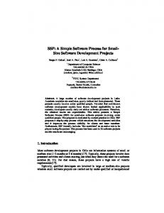
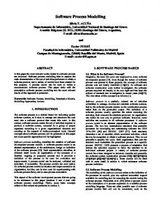
schedule overrun is only 4%. Also, in Run 6, the schedule underrun is 5%, whereas in Run 9, it is 9%. These runs also indicate that attrition costs more when it occurs later in the project. The results in Table 4 may also be viewed as an evaluation of three staffing strategies for attrition in five sets of the three factors. Each set is comprised of (number of engineers, increment number ending at time of attrition, and attrition rate). Because we are considering three factors in this experiment, the orthogonal relationships of these five sets of factors are illustrated in the cube of Figure 3. When the staffing strategy for attrition is compared within each set of factors, desirable strategies can be identified based on cost and project duration against the estimated schedule. These results are summarized in Figure 4, which adds the desirable strategies to the cube of Figure 3. In Figure 4, N represents the strategy of no replacement and no overstaffing, R represents the replacement strategy, and O represents the overstaffing strategy. In some situations either of two strategies is desirable, depending on whether one wishes to minimize cost or complete the project on
schedule (or in the N for cost (20,2,10) case, (10,2,30) minimize the R for schedule Increment no. schedule overrun). For e x a m p l e , completed point (10,1,10) in at time of Figure 4 represents a attrition N for cost (20,2,10) project in which the O for schedule ratio of estimated effort to the number of Attrition rate engineers is high (say finish about 3% (10,1,30) early but will add N for cost about 1% to the cost R for schedule of the project. Overstaffing to anticipate this (10,1,10) attrition will allow (20,1,10) R N No. of engineers the project to complete about 4% early and will increase the project cost about 4%. The
As another example, in the case of 20 engineers on the project and two people leave at the end of increment 2 (point (20,2,10) in Figure 4), other schedule regardless of the chosen course of action, but overstaffing (O) will limit the overrun. Neither
900 hours) and one person leaves at the end of Increment 1. In this scenario, the project can finish on-time without replacing the person. Replacing the person will allow the project to most desirable strategy for this set of factors, then, is no action (N) because it allows the project to finish on time at the lowest cost.
strategies are indicated. The project will overrun the estimated replacing nor overstaffing (N) remains the best option for minimizing cost.
Figure 3. Relationships of Factor Sets in Table 2.
Figure 4. Desirable Staffing Strategies for Attrition under Each Set of Factors most influential factors for modeling software dynamics and, more importantly, their degrees of Conclusions and Future Research influence on project outcomes. Our research grew out of the concern for having strategies to address attrition in software development organizations. We also wished to examine the ability of a more abstract simulator, composed of four process feedback loops, to provide realistic data for supporting the formulation of staffing policies. This experiment suggests several implications for software project staffing in response to attrition. In general, no action for attrition is the least expensive choice and overstaffing is the most expensive choice. The choice of no action is indicated when schedule pressure is high and cost containment is a priority. The replacement strategy has the advantage of alleviating the exhaustion rate and concomitant increases in attrition. Even though overstaffing is the more expensive option, it can have the very desirable effect of minimizing project duration. Thus, this strategy should be considered for projects in which completion date has been identified as the highest priority. Such a circumstance might occur if delivery of a commercial application is required during a market "window of opportunity," or if the contract for a custom application has a penalty attached to late delivery. The cost of overstaffing must be weighed with the other factors in the project and process simulation can provide data for this decision. Regarding process modeling objectives and the use of SDM, this experiment has demonstrated the use of a software development process simulator, one which models the major dynamic influences in a project. The software practitioners who examined the results produced by this experiment found them to be both acceptable and realistic. This model is capable of supporting designed experimentation and providing data for supporting staffing decisions. This group continues to research in software development process simulation. In addition to the questions of attrition, the group continues investigating into questions related to project management training, project risk assessment, and product quality. In terms of process modeling issues, further research continues to identify and validate the
References [1] Abdel-Hamid, Tarek, A Study of Staff Turnover, "Acquisition, and Assimilation and Their Impact on Software Development Cost and Schedule", Journal of Manager Information Systems, Summer 1989, vol. 6, no. 1, pp. 21-40. [2] Abdel-Hamid, Tarek and Stuart E. Madnick, Software Project Dynamics An Integrated Approach, PrenticeHall, Englewood Cliffs, New Jersey, 1991. [3] Abdel-Hamid, Tarek, "Thinking in Circles", American Programmer, May 1993, pp. 3-9. [4] Bevilaqua, Richard J. and D.E. Thornhill, "Process Modeling", American Programmer, May 1992, pp. 3-9. [5] Collofello, James S., J. Tvedt, Z. Yang, D. Merrill, and I. Rus, "Modeling Software Testing Processes", Proceedings of Computer Software and Applications Conference (CompSAC'95), 1995. [6] Curtis, Bill, M. I. Kellner and J. Over, "Process Modeling", Communications of the ACM, 35(9), Sept. 1992, pp. 75-90. [7]ithink Manual, High Performance Systems, Inc., Hanover, NH, 1994. [8] Lin, Chi Y., "Walking on Battlefields: Tools for Strategic Software Management", American Programmer, May, 1993, pp. 34-39. [9] Madachy Raymond, "System Dynamics Modeling of an Inspection-based Process", Proceedings of the Eighteenth International Conference on Software Engineering, Berlin, Germany, March 1996.
[10] Richardson, George P. and Alexander L. Pugh III, Introduction to System Dynamics Modeling with DYNAMO, The M.I.T. Press, Cambridge, MA, 1981. [11] Richmond, Barry, "System Dynamics/Systems Thinking: Let's Just Get On With It", International System Dynamics Conference, Sterling, Scotland, 1994. [12] Rubin, Howard A., M. Johnson and Ed Yourdon, "With the SEI as My Copilot Using Software Process "Flight Simulation" to Predict the Impact of Improvements in Process Maturity", American Programmer, September 1994, pp. 50-57. [13] Smith, Bradley J, N. Nguyen and R. F. Vidale, "Death of a Software Manager: How to avoid Career Suicide
through Dynamic Software Process Modeling", American Programmer, May 1993, pp. 11-17. [14] Sycamore, Douglas M., Improving Software Project Management Through System Dynamics Modeling, Master of Science Thesis, Arizona State University, 1996. [15] Tvedt, John D., An Extensible Model for Evaluating the Impact of Process Improvements on Software Development Cycle Time, Ph.D. Dissertation, ASU, 1996. [16] Beagley, S.M., “Staying the Course with the Project Control Panel.” American Programmer (March 1994) 29-34.