Hindawi Publishing Corporation Mobile Information Systems Volume 2016, Article ID 2098927, 11 pages http://dx.doi.org/10.1155/2016/2098927
Research Article A TDoA Localization Scheme for Underwater Sensor Networks with Use of Multilinear Chirp Signals En Cheng, Xizhou Lin, Shengli Chen, and Fei Yuan Key Laboratory of Underwater Acoustic Communication and Marine Information Technology (Xiamen University), Ministry of Education, Xiamen 361005, China Correspondence should be addressed to Fei Yuan;
[email protected] Received 22 July 2016; Accepted 7 September 2016 Academic Editor: Hyun-Ho Choi Copyright © 2016 En Cheng et al. This is an open access article distributed under the Creative Commons Attribution License, which permits unrestricted use, distribution, and reproduction in any medium, provided the original work is properly cited. Due to the multipath, Doppler, and other effects, the node location signals have high probability of access collision in the underwater acoustic sensor networks (UW-ASNs), and therefore, it causes the signal lost and the access block; therefore, it constrains the networks performance. In this paper, we take the multilinear chirp (MLC) signals as the location signal to improve the anticollision ability. In order to increase the detection efficiency of MLC, we propose a fast efficient detection method called mixing change ratefractional Fourier transform (MCR-FrFT). This method transforms the combined rates of MLC into symmetry triangle rates and then separates the multiuser signals based on the transformed rates by using FrFT. Theoretical derivation and simulation results show that the proposed method can detect the locations signals, estimate the time difference of arrival (TDoA), reduce the multiple access interference, and improve the location performance.
1. Introduction During the last couple of years, we could observe a growing interest in underwater acoustic sensor networks (UWASNs). One important reason is that the UW-ASNs improve ocean exploration ability and fulfill the needs of a multitude of underwater applications, including oceanographic data collection, warning systems for natural disasters, ecological applications, military underwater surveillance, assisted navigation, and industrial applications. However, the location of the sensors needs to be determined because sensed data can only be interpreted meaningfully when referenced to the location of the sensor. Due to the absorption of electromagnetic wave, the well-known Global Position System (GPS) receivers, which may be used in terrestrial systems to accurately estimate the geographical locations of sensor nodes, could not work properly underwater [1]. Therefore, localization for UW-ASNs has been one of the major research topics since UW-ASNs started to draw the attention of the networking community in the early 2000s [2]. Sensors’ self-localization is the basic and key requirement for the self-organization of UW-ASNs. It can be achieved
by leveraging the low speed of sound in water to accurately determine the internode distance [3]. Localization of underwater equipment has also been an essential part of the traditional oceanographic systems where it has been established by one of two techniques: short base line (SBL) [4] or long base line (LBL) [5]. Time difference of arrival (TDoA) method is typically used in LBL systems. In TDoAbased localization, the difference in the measured time of arrivals of signals, received from a pair of reference nodes, is translated to the difference in range estimates with those reference nodes and gives rise to a hyperbola for the unknown position of the node (target node). A unique estimation of the target node position can be obtained by intersecting three such hyperbolas. However, this technique requires that reference nodes transmit at near concurrent time because of the water currents (the motion of the target node). Traditional LBL systems are designed for small deployments consisting of a few reference nodes (here called beacons), whose acoustic transmissions can be received by all submersibles within the deployment. LBL provides sufficient localization accuracy for such deployments. This is because signals from few beacons can be scheduled to occur within a
2
Mobile Information Systems
short time window. Since all the target nodes are within the communication range of the beacons, these signals also arrive at near concurrent times at each target node. Therefore, the TDoA is suitable. However, as the spatial extent and the size of the system are scaled up, the number of location signals increases too. Therefore, to avoid location signals’ collision is also urgent, within the short time window.
2. Related Works Acoustic-based localization was studied because of its application in underwater sensor networks localization. In [6], a TDoA-based silent positioning algorithm termed as UPS for UW-ASNs was proposed. In [7], the localization problem in sparse 3D underwater sensor networks was studied based on TDoA. In [8], a TDoA for multiple acoustic sources in reverberant environments was proposed, and the ambiguities in the TDoA estimation caused by multipath propagation and multiple sources were resolved by exploiting two TDoA constraints: the raster condition and the zero cyclic sum condition. However, these references do not consider the collisions of location signals in the target sensor. In [9], a different system where transmissions from multiple reference nodes have to be sufficiently lagged over a time epoch to avoid collisions was presented, but it needs a lot of time to localize the target sensor. In [10], the authors introduced a method for designing localization signal based on Code Division Multiple Access (CDMA), and the modulation mode is ASK; but as described in [11] about the physical layer of underwater channel, ASK modulation is not suitable for underwater channel because of high attenuation. What is more, the location signals are transmitted that are sufficiently lagged, which is the same as [9]. In [8], to avoid collisions and meet the signal concurrency requirement of traditional LBL systems simultaneously, a TDoA location scheme for the orthogonal frequency division multiplexing (OFDM) was presented; this outperforms the location schemes with traditional TDoA estimations. Unfortunately, the OFDM system is very sensitive to Doppler, which is one of the main characters of underwater channel. In [11, 12], a time-varying multichirp rate modulation for multiple access systems was used to avoid collision in terrestrial communication. Chirp signal is widely used in underwater acoustic communication [13], because it is robust to channel noise and resistant to multipath fading [14] and has low Doppler sensitivity [13]. Some different methods are used to estimate the parameters of chirp signal. In [12], the method of time-delay frequency mixing (rate reduction) to convert the chirp signal with different chirp rate into MFSK signal is proposed, but it is not suited for combined chirp signal because of the change of chirp rate. In [11, 12], the detection technique of matched filter receiver (correlation method) was mentioned, but it is difficult and also needs amplitude modulation which is not suitable for underwater channel. The fractional Fourier transform (FrFT) presents best localization performance in a certain FrFT domain, which is useful for the detection and estimation of multicomponent linear frequency modulation (LFM) signals [15] and some improved algorithms based on FrFT are also proposed, such as EEMD-FrFT [16] and
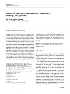
Communication link Reference node Unknown node
Figure 1: Location system architecture using combined chirp signals.
STFT [17]; they overcome some disadvantages such as high computation cost for combined chirp signals. In this paper, a method called mixing change rate-FrFT (MCR-FrFT) is proposed to deal with the drawback. In this paper, a TDoA location scheme using the multilinear chirp modulation signals (called MLC signals) is proposed for UW-ASNs. The rest of the paper is organized as follows: in Section 3, the system model and location signals are described. In Section 4, we analyze the system with the underwater environment in TDoA estimation. In Section 5, we present our simulation results on our passive localization scheme for the multilinear chirp signals. Section 6 concludes this paper.
3. System Model The system architecture of the scheme is depicted in Figure 1. The white nodes are reference nodes whose locations are known, while the black node is target node which needs to be located. Arrows indicate the communication links. The system is designed to work with only one-way reference node transmissions. The reference nodes and target node are fully synchronized with each other and the target node is within the communication range of at least four reference nodes (3D network) or three reference nodes (2D network). Since the communication range and distance between reference nodes are all hundred meters’ scale, the location signals get high possibility to arrive at the same time. Therefore, avoiding collision is a key problem to node localization. We introduce the chosen location signal and the processing of the signal in the following subsections. 3.1. Location Signal-Multilinear Chirp (MLC) Signal. Due to the match of MLC and underwater channel, the MLC is chosen as the location signal, and its time-frequency characteristic of location signals-MLC is shown as Figure 2, where 𝑇 is the duration time of location signal. Nodes are
Mobile Information Systems
3
T/2
f 2M 2M − 1
𝜇𝑚𝑓 = 2
(𝑚 − 2𝑀 − 1) 𝐵 , (𝑀 + 1) 𝑇
𝜇𝑚𝑏 = 2
(𝑚 − 𝑀) 𝐵 , (𝑀 + 1) 𝑇
1 2
(5) 𝑚 ∈ (𝑀, 2𝑀] .
As shown in Figure 2, each location signal has the same bandwidth 𝐵 and duration time 𝑇; thus the system produces equal time-bandwidth product 𝐷 = 𝐵𝑇 for all nodes. Equal 𝐷 makes the nodes in the UW-ASNs have the equal position, which is important for mobile nodes.
B
M−1
M+2
M
M+1 T
t
Figure 2: The time-frequency characteristic of location signals.
denoted by 1, 2, . . . , 𝑀, 𝑀+1, . . . , 2𝑀−1, 2𝑀, where the first 𝑀 nodes are with positive combined slopes and the second 𝑀 nodes are with negative combined slopes. Each signal is composed of two segments with two different slopes. The signal for 𝑚th node is expressed as 𝑆𝑚 (𝑡) = 𝑆𝑚𝑓 (𝑡) + 𝑆𝑚𝑏 (𝑡) .
(1)
Subscripts 𝑓 and 𝑏 indicate the first half and the second half of duration time 𝑇, respectively. And 𝑆𝑚𝑓 (𝑡) = 𝐴 exp (𝑗𝜋𝜇𝑚𝑓 𝑡2 ) ⋅ exp (𝑗2𝜋𝑓𝑐 𝑡) ,
(2)
𝜇𝑚𝑓
𝑇 ⋅ exp (𝑗2𝜋 (𝑓𝑐 + 𝑇) (𝑡 − )) , 2 2
(3)
where 𝑓𝑐 is the carrier frequency, 𝑚 is the node number, 𝑚 = 1, 2, . . . , 𝑀, . . . , 2𝑀, 𝐴 is the amplitude of signal, and 2𝑀 is the total number of nodes in UW-ASNs. 𝜇𝑚𝑓 is 𝑚th node’s slope within the first half of signal duration and 𝜇𝑚𝑏 is the slope of 𝑚th node within the second half of signal duration. The slopes of general combined chirp signal can be expressed as (𝑀 + 1 − 𝑚) 𝐵 , (𝑀 + 1) 𝑇
𝜇𝑚𝑏 = 2
𝑚𝐵 , (𝑀 + 1) 𝑇
(4) 𝑚 ∈ [1, 𝑀] ,
𝑥local (𝑡)
(6)
𝑟0 (𝑡) = 𝑟𝑓 (𝑡) ∗ ℎLPF (𝑡) , 𝑟𝑓 (𝑡) = 𝑟 (𝑡) ⋅ 𝑥local (𝑡) ,
when 𝑇/2 ≤ 𝑡 < 𝑇,
𝜇𝑚𝑓 = 2
3.2.1. Mixing Change Rate (MCR). The purpose of MCR is to change the chirp rates of MLC signals into a new set of rates. It includes two parts, multiplier and low pass filter. The block diagram of MCR is shown in Figure 3(b):
𝐵 2 { {𝑥local𝑢 (𝑡) = exp (𝑗𝜋 𝑇 𝑡 ) ⋅ exp (𝑗2𝜋𝑓𝑐 𝑡) , ={ 𝐵 { 𝑥local𝑑 (𝑡) = exp (−𝑗𝜋 𝑡2 ) ⋅ exp (𝑗2𝜋𝑓𝑐 𝑡) , { 𝑇
when 0 ≤ 𝑡 < 𝑇/2, and 𝑇 2 𝑆𝑚𝑏 (𝑡) = 𝐴 exp (𝜋𝜇𝑚𝑏 (𝑡 − ) ) 2
3.2. Detection Block Diagram and Principle. The localization signal detection problem could be described as deciding which one of the 2M possible signals was transmitted, given the received signal during the interval time of (0, 𝑇). The method of parameter estimation proposed in the paper is called MCR-FrFT, whose block diagram is shown as Figure 3(a). The received signal is divided into two branches. Each branch has its own local signals 𝑥local𝑢(𝑡) and 𝑥local𝑑(𝑡), respectively, 𝑥local𝑢(𝑡) for the up branch (𝑚 ≤ 𝑀) and 𝑥local𝑑(𝑡) for the down branch (𝑀 < 𝑚 ≤ 2𝑀).
where ℎLPF (𝑡) is the impulse response function of low pass filter (LPF). Assuming that 𝑚th node’s signal is received and 𝑚 < 𝑀, we get the received signal as (7) by substituting (2)– (4) into (1). 𝑛(𝑡) is the underwater acoustic channel noise. After the MCR, the high frequency terms have been filtered out and the received signal becomes as (8) and 𝑤(𝑡) = (𝑛(𝑡) ⋅ 𝑥local(𝑡)) ∗ ℎLPF (𝑡). The frequency and time relationship of received signals after multiplier (𝑟𝑓 ) are shown in Figure 4. From the figure, 𝑚th location signal, composed of two different positive slopes, is changed into two branches of new multilinear chirp signals. The up branch (𝑚 ≤ 𝑀) has chirp rates of positive and negative relationship, while the down branch (𝑀 < 𝑚 ≤ 2𝑀) is composed of another chirp rate. However, the received signal only has the up branch after being filtered in the LPF of MCR:
4
Mobile Information Systems
MCR
Received signal
BPF
r(t)
r0 (t)
s0 (t)
FrFT
Decision
(xlocalu(t)) MCR
User m (m ≤ M) r(t)
r0 (t)
s0 (t)
FrFT
(xlocald(t))
Decision
User m (m > M)
rf (t)
LPF
r0 (t)
xlocal(t)
(a)
(b)
Figure 3: System block diagram. (a) The detection block diagram. (b) The block diagram of MCR.
𝑟 (𝑡) = 𝑆𝑚 (𝑡) + 𝑛 (𝑡) = 𝐴 exp (𝑗𝜋𝜇𝑚𝑓 𝑡2 ) ⋅ exp (𝑗2𝜋𝑓𝑐 𝑡) ⋅ rect (
𝜇𝑚𝑓 4𝑡 − 𝑇 𝑇 2 𝑇 4𝑡 − 3𝑇 ) + 𝐴 exp (𝑗𝜋𝜇𝑚𝑏 (𝑡 − ) ) ⋅ exp (𝑗2𝜋 (𝑓𝑐 + 𝑇) (𝑡 − )) ⋅ rect ( ) 2𝑇 2 2 2 2𝑇
(7)
+ 𝑛 (𝑡) , 𝑟0 (𝑡) = 𝑤 (𝑡) +
𝐴2 2
{ { { {cos (𝜋 (𝜇𝑚𝑓 − ⋅{ { { {cos (𝜋 (𝜇𝑚𝑓 + {
𝐵 2 4𝑡 − 𝑇 𝑀+1−𝑚 ) 𝑡 ) ⋅ rect ( ) + cos [2𝜋 ( 𝐵− 𝑇 2𝑇 𝑀+1 𝐵 2 4𝑡 − 𝑇 𝑀+1−𝑚 ) 𝑡 ) ⋅ rect ( ) + cos [2𝜋 ( 𝐵+ 𝑇 2𝑇 𝑀+1
𝐵 4𝑡 − 3𝑇 𝐵 𝑇 𝑇 2 ) (𝑡 − ) + 𝜋 (𝜇𝑚𝑏 − ) (𝑡 − ) ] ⋅ rect ( ), 𝑚 ≤ 𝑀, 2 2 𝑇 2 2𝑇 2 𝐵 4𝑡 − 3𝑇 1 𝑇 𝑇 𝐵) ⋅ (𝑡 − ) + 𝜋 (𝜇𝑚𝑏 + ) (𝑡 − ) ] ⋅ rect ( ) , 𝑀 < 𝑚 ≤ 2𝑀. 2 2 𝑇 2 2𝑇
3.2.2. Fractional Fourier Transform (FrFT). FrFT is a generalized Fourier transformation form and it can be regarded as the Fourier transform to 𝑝th order, where 𝑝 needs not be an integer; thus it can transform a function to any intermediate domain between time and frequency [18]. For signal 𝑥(𝑡), the FrFT has the following form:
𝑋𝑝 (𝑢) = ∫
+∞
−∞
𝑟 (𝑡) = 𝐴 0 cos (2𝜋𝑓𝑐 𝑡 + 𝜋𝑢𝑡2 ) + 𝑛 (𝑡) ,
(11)
where 0 ≤ 𝑡 ≤ 𝑇 and 𝑛(𝑡) is white noise. The FrFT of 𝑟(𝑡) is +∞
𝑋𝑝 (𝑢) = ∫
−∞
= 𝐴 0√
𝑟 (𝑡) 𝐾𝑝 (𝑡, 𝑢) 𝑑𝑡 1 − 𝑗 cot 𝛼 (𝑗(1/2)𝑢2 cot 𝛼) 𝑒 2𝜋
(9)
and the transform kernel is
1 − 𝑗 cot (𝛼) 1 1 { { √ exp [𝑗 ( 𝑡2 cot (𝛼) + 𝑢2 cot (𝛼) − 𝑡𝑢 csc (𝛼))] , { { 2𝜋 2 2 { 𝐾𝑝 (𝑡, 𝑢) = {𝛿 (𝑡 − 𝑢) , { { { { {𝛿 (𝑡 + 𝑢) ,
where 𝑝 is the transform order, 𝛼 is the angle of rotation, and 𝛼 = 𝑝𝜋/2. When 𝑝 = 1, FrFT will degenerate into Fourier transformation, and when 𝑝 = 0, FrFT is just the original signal. Simple component LFM signal with noise has the following form:
𝐾𝑝 (𝑡, 𝑢) 𝑥 (𝑡) 𝑑𝑡,
(8)
𝑇
⋅ ∫ 𝑒(2𝑗𝜋((1/2)𝑡
𝛼 ≠ 𝑛𝜋, (10)
𝛼 = 2𝑛𝜋, 𝛼 = (2𝑛 ± 1) ,
2
(𝑢+cot 𝛼/2𝜋)+𝑡(𝑓𝑐 −𝑢 csc 𝛼/2𝜋)))
0
𝑑𝑡
𝑇
+ ∫ 𝑛 (𝑡) 𝐾𝑝 (𝑡, 𝑢) 𝑑𝑡. 0
(12) In (12), the LFM signal is an impulse function only in the appropriate fractional Fourier domain. The amplitude of energy aggregation of LFM signal will exhibit obvious peak by doing an appropriate 𝑝-order FrFT, while the noise, which cannot appear in energy aggregation at any fractional Fourier domain, is distributed on the whole time-frequency plane evenly. Figure 4 shows that the set of chirp rates is changed from two different slopes, which needs two different 𝑝 values to complete its parameter estimation, to a new set of chirp rates
Mobile Information Systems
5 According to (4) and (8), there are different sets of chirp rates included in the MCR results with different 𝑚, 𝑛, 𝑙 group:
The new set of chirp rates by MCR 10000 9000 8000
𝑟0 (𝑡) =
Frequency (Hz)
7000 6000 5000 4000 3000
+ cos (𝜋
(𝑀 + 1 − 2𝑙) 𝐵 2 𝑡) (𝑀 + 1) 𝑇
+ cos (𝜋
4𝑡 − 𝑇 (𝑀 + 1 − 2𝑛) 𝐵 2 ) 𝑡 )] ⋅ rect ( 2𝑇 (𝑀 + 1) 𝑇
2000
+
1000 0
0
0.005
0.01
0.015
0.02 0.025 Time (s)
0.03
0.035
0.04
User 1, original set User 1, up branch User 1, down branch
𝐴2 𝑀+1−𝑚 𝐵 𝑇 [cos (2𝜋 ( 𝐵 − ) (𝑡 − ) 2 𝑀+1 2 2
−𝜋
−𝜋 that the new two slopes are with same absolute value but one positive and one negative by using the MCR. At this condition, only one value needs to complete the parameter estimation, that is, one FrFT for a single branch, while two FrFT are needed for the scheme of FrFT (without MCR). Since FrFT cost more computation than the MCR module, our MCR-FrFT saves computations of system. In practical application, the discrete fractional Fourier transform (DFrFT) is usually used.
4. TDoA Estimation There are two steps of MCR-FrFT at the receiving end. In the first step, MCR takes effect to convert the chirp rates of location signal into a new set of chirp rates. Then, FrFT estimates the parameters. There are two parameters considered: chirp rate, which represents the reference node, and initial frequency, which can be used for estimation of the processing delay. 4.1. Collision Avoidance. One of the advantages of the paper is to avoid collision. Taking an example with three reference nodes 𝑚, 𝑙, 𝑛 ∈ [1, 𝑀], 𝑟 (𝑡) = 𝑆𝑚 (𝑡) + 𝑆𝑙 (𝑡) + 𝑆𝑛 (𝑡) + 𝑛 (𝑡) .
(13)
𝜌𝑙,𝑚 =
𝑇 2 (𝑀 + 1 − 2𝑙) 𝐵 (𝑡 − ) ) 2 (𝑀 + 1) 𝑇
+ cos (2𝜋 ( −𝜋
√|𝑙−𝑚|𝐵𝑇/4(𝑀+1)
𝐴 (𝑀 + 1) [ √ ∫ 4 |𝑙 − 𝑚| 𝐵𝑇 0 [
cos (2𝜋V2 ) 𝑑V
(14)
𝑀+1−𝑙 𝐵 𝑇 𝐵 − ) (𝑡 − ) 𝑀+1 2 2
𝑀+1−𝑛 𝐵 𝑇 𝐵 − ) (𝑡 − ) 𝑀+1 2 2
4𝑡 − 3𝑇 𝑇 2 (𝑀 + 1 − 2𝑛) 𝐵 ) (𝑡 − ) )] ⋅ rect ( 2 2𝑇 (𝑀 + 1) 𝑇
+ 𝑤 (𝑡) . From (14), we could see that the performance of MLC signals mainly depends on the cross-coherence between the different location signals even by passing the MCR. Ideally, the signals should be orthogonal with zero cross-coherence to cancel the multiple access interference. Set 𝐴 = √2𝐸/𝑇, where 𝐸 is the signal energy in the whole duration, and the cross-correlation of signals 𝜌 takes the following form:
𝜌𝑙,𝑚 =
1 𝑇 ∗ ∫ 𝑆 (𝑡) ⋅ 𝑆𝑚 (𝑡) 𝑑𝑡. 𝐸 0 𝑙
(15)
Substituting the corresponding values of 𝑆(𝑡) in (13) and neglecting the integration over the higher frequencies, we get
𝑇/2 𝑇 𝑇 2 𝐴4 𝑙−𝑚 𝑇 𝑙−𝑚 (𝑙 − 𝑚) 𝐵 2 ) 𝑡 𝑑𝑡 + ∫ cos (2𝜋 𝐵 (𝑡 − ) ) 𝑑𝑡] . [∫ cos (2𝜋 𝐵 (𝑡 − ) − 2𝜋 8𝐸 0 𝑀+1 2 2 (𝑀 + 1) 𝑇 (𝑀 + 1) 𝑇 𝑇/2
Take V = √|𝑙 − 𝑚|𝐵/(𝑀 + 1)𝑇𝑡, 𝑢 = √|𝑙 − 𝑚|𝐵/(𝑀 + 1)𝑇(𝑡 − 𝑇/2); then (16) can be changed to 2
𝑇 2 (𝑀 + 1 − 2𝑚) 𝐵 (𝑡 − ) ) 2 (𝑀 + 1) 𝑇
+ cos (2𝜋 (
Figure 4: The time-frequency characteristic after MCR.
𝜌𝑙,𝑚 =
𝐴2 (𝑀 + 1 − 2𝑚) 𝐵 2 [cos (𝜋 𝑡) 2 (𝑀 + 1) 𝑇
+∫
√|𝑙−𝑚|𝐵𝑇/4(𝑀+1)
0
=
(16)
|𝑙 − 𝑚| 𝐵𝑇 cos (2𝜋√ 𝑢 − 2𝜋𝑢2 ) 𝑑𝑢] 𝑀+1 ]
𝐴2 √ (𝑀 + 1) √(Δ𝑛⋅𝐷)/4(𝑀+1) cos (2𝜋𝑡2 ) 𝑑𝑡 ∫ 4 Δ𝑛 ⋅ 𝐷 0
6
Mobile Information Systems M = 30, l-m = 2
0.9
0.2
0.8
0.18
0.7
0.16
0.6 0.5 0.4
0.14 0.12 0.1
0.3
0.08
0.2
0.06
0.1
0
10
20
30
D = 100, l-m = 2
0.22
Cross-coherence
Cross-coherence
1
40 50 60 70 Time-produce (D)
80
90
0.04
100
0
10
20 30 40 Total number of nodes (M)
(a)
50
60
(b)
M = 30, D = 100, l-m = N
0.25
Cross-coherence
0.2
0.15
0.1
0.05
0
0
5
10
15 20 Node interval (N)
25
30
(c)
Figure 5: Cross-coherence function 𝜌 as a function of (a) time-bandwidth product with 𝑀 = 30 and Δ𝑛 = 2. (b) Total node numbers 𝑀 with 𝐷 = 100 and Δ𝑛 = 2. (c) User difference with 𝑀 = 30 and 𝐷 = 100.
+ cos (2𝜋√
Δ𝑛 ⋅ 𝐷 𝑡 − 2𝜋𝑡2 ) 𝑑𝑡, 𝑀+1 (17)
where 𝐷 = 𝐵𝑇 is time-bandwidth product and 𝑙−𝑚 = Δ𝑛. We could see that 𝜌 has an oscillatory nature as a function of 𝐷, 𝑀, and Δ𝑛, due to the Fresnel function form of (17). Usually, smaller cross-correlation 𝜌 indicates a better performance of the system. The normalized sample values can be expressed as
𝜌𝑀×𝑀
1 [𝜌 [ 21 [ =[ . [ . [ .
𝜌1,2 ⋅ ⋅ ⋅ 𝜌1,𝑀 1 .. .
⋅ ⋅ ⋅ 𝜌2,𝑀] ] ] , .. ] ] . ]
[𝜌𝑀,1 𝜌𝑀,2 ⋅ ⋅ ⋅
1 ]
(18)
where 𝜌𝑖,𝑗 is the cross-coherence between 𝑖th and 𝑗th location signal and number 1 on the matrix diagonal represents the location signal itself. Figure 5 shows that the cross-coherence is an oscillatory function of time-bandwidth product 𝐷 or the total number of MLC signals or the difference between chirp rates Δ𝑛, when the other two parameters are set fixed. Figure 5(a) indicates that 𝜌 decreases oscillatorily as 𝐷 increases when 𝑀 = 30 and Δ𝑛 = 2. Figure 5(b) indicates that 𝜌 increases oscillatorily as 𝑀 increases when 𝐷 = 100 and Δ𝑛 = 2. Figure 5(c) indicates that 𝜌 decreases oscillatorily as Δ𝑛 increases when 𝐷 = 100 and 𝑀 = 30. We could select the assembling parameter according to (17) in practice. 4.2. The Result of Underwater Channel. The impulse response of an underwater acoustic channel is influenced by the geometry of the channel and its reflection properties, which determine the number of significant propagation paths, their
Mobile Information Systems
7
relative strengths, and delays. Strictly speaking, there are infinitely many signal echoes, but those that have undergone multiple reflections and lost much of the energy can be discarded, leaving only a finite number of significant paths. At this point, the channel impulse response can be expressed as 𝑁−1
ℎ (𝑡) = 𝐴 0 𝛿 (𝑡 − 𝜏0 ) + ∑ 𝐴 𝑖 𝛿 (𝑡 − 𝜏𝑖 ) ,
where 𝑁 is the total number of propagation paths, and 𝑖 = 0 corresponding to the direct path, 𝐴 𝑖 is the amplitude of 𝑖th propagation path at receiving side, and 𝜏𝑖 is the propagation delay of 𝑖th propagation path. Assuming that the transmitted signal is 𝑠(𝑡), then the received signal 𝑟(𝑡) can be expressed as 𝑁−1
𝑟 (𝑡) = 𝐴 0 𝑠 (𝑡 − 𝜏0 ) + ∑ 𝐴 𝑖 𝑠 (𝑡 − 𝜏𝑖 ) + 𝑛 (𝑡) (20)
𝑁−1
−𝜋
(𝑀 + 1 − 2𝑚) 𝐵𝑇 − 4𝑚𝐵𝜏𝑖 𝑇 (𝑡 − ) 2 (𝑀 + 1) 𝑇 2
𝑇 2 (𝑀 + 1 − 2𝑚) 𝐵 (𝑡 − ) 2 (𝑀 + 1) 𝑇
− 2𝜋
(𝑀 + 1 − 𝑚) 𝐵𝜏𝑖 − 2𝜋𝑓0 𝜏𝑖 𝑀+1
+ 2𝜋
4 (𝑡 − 𝜏𝑖 ) − 3𝑇 𝑚𝐵 ). 𝜏 2 )] ⋅ rect ( 2𝑇 (𝑀 + 1) 𝑇 𝑖
(19)
𝑖=1
𝑖=1
+ [cos (2𝜋
(23) From the above equations, we could see that the frequencies of combined chirp signal are changed due to the Doppler, but the sets of chirp rates for different nodes are unchanged. Since our location signals are detected according to the different sets of chirp rates, which is only determined by 𝑚th order for the fixed system, the MLC signals would not be affected by multipath properties of underwater acoustic channel.
= ∑ 𝐴 𝑖 ⋅ 𝑠 (𝑡 − 𝜏𝑖 ) + 𝑛 (𝑡) . 𝑖=0
Taking the Doppler into account, let 𝑠(𝑡) = 𝑆𝑚 (𝑡); then the received signal can be expressed as 𝑁−1
𝑟 (𝑡) = ∑ 𝐴 𝑖 ⋅ 𝑆𝑚 (𝑡 − 𝜏𝑖 ) ⋅ exp (𝑗2𝜋𝜀𝑖 (𝑡 − 𝜏𝑖 )) + 𝑛 (𝑡) 𝑖=0
𝑁−1
2
= ∑ 𝐴 𝑖 [cos (2𝜋𝑓0 (𝑡 − 𝜏𝑖 ) + 𝜋𝜇𝑚𝑓 (𝑡 − 𝜏𝑖 ) ) 𝑖=0
⋅ rect (
4 (𝑡 − 𝜏𝑖 ) − 𝑇 ) 2𝑇
+ cos (2𝜋 (𝑓0 +
𝑇 (𝑀 + 1 − 𝑚) 𝐵) (𝑡 − 𝜏𝑖 − ) 𝑀+1 2
+ 𝜋𝜇𝑚𝑏 (𝑡 − 𝜏𝑖 −
4 (𝑡 − 𝜏𝑖 ) − 3𝑇 𝑇 2 ) ) ⋅ rect ( )] 2 2𝑇
(21)
⋅ exp (𝑗2𝜋𝜀𝑖 (𝑡 − 𝜏𝑖 )) + 𝑛 (𝑡) . Substituting the corresponding values into (21), neglecting the third branch, and using MCR we get 1𝑁 𝑟0 (𝑡) = ∑𝐴 𝑖 𝑋 (𝑡) ⋅ exp (𝑗2𝜋𝜀𝑖 (𝑡 − 𝜏𝑖 )) + 𝑤 (𝑡) , 2 𝑖=1 where 2 (𝑀 + 1 − 𝑚) 𝐵𝜏𝑖 𝑡 𝑋 (𝑡) = [cos (2𝜋 (𝑀 + 1) 𝑇 −𝜋
(𝑀 + 1 − 2𝑚) 𝐵 2 𝑡 + 2𝜋𝑓0 𝜏 (𝑀 + 1) 𝑇
− 2𝜋
4 (𝑡 − 𝜏𝑖 ) − 𝑇 (𝑀 + 1 − 𝑚) 𝐵 2 ) 𝜏𝑖 )] ⋅ rect ( 2𝑇 (𝑀 + 1) 𝑇
(22)
4.3. Positioning Process. The target node receives the location signals and determines the corresponding reference node with time (𝑡𝑚 , 𝑡𝑙 , 𝑡𝑛 ) and position (𝑥𝑚 , 𝑦𝑚 ), (𝑥𝑙 , 𝑦𝑙 ), (𝑥𝑛 , 𝑦𝑛 ), when and where the location signal was transmitted. In this system, the location signals are received at the same time so the difference between 𝑡𝑚 and 𝑡𝑙 is a constant; in other words, the difference between the corresponding distance 𝑟𝑚 and 𝑟𝑙 is a constant. Of course, |𝑟𝑚 − 𝑟𝑛 | and |𝑟𝑙 − 𝑟𝑛 | are constants too. Based on the property of hyperbola, the target node is localized by the intersection of three curves as shown in Figure 6. In Figure 6, 𝑐 is the speed of sound in underwater channel in m/s. Hyperbolic curve 𝐻𝑙,𝑛 is determined by nodes 𝑙 and 𝑛, while 𝐻𝑚,𝑛 and 𝐻𝑙,𝑚 are determined by 𝑚, 𝑛 and 𝑙, 𝑛 respectively. For this system, the scaling parameter and the length of interval are 𝑆 = (𝑇/𝑓𝑠 )1/2 = 𝑁1/2 /𝑓𝑠 and Δ𝑥 = (𝑇𝑓𝑠 )1/2 = 𝑁1/2 , respectively, where 𝑁 = 𝑓𝑠 ⋅ 𝑇 is the sample number. When 𝑝 = 𝑝0 is the optimal 𝑝 order, then there are two different energy accumulation peaks (assuming that the coordinates are 𝑚01 and 𝑚02 ) symmetrical about 𝑁/2 that are got. 𝑚01 = 𝑚02
𝑁 + Δ𝑥 ⋅ 𝑓𝑖 ⋅ 𝑆 ⋅ sin (𝛼0 ) , 2
𝑁 = − Δ𝑥 ⋅ 𝑓𝑖 ⋅ 𝑆 ⋅ sin (𝛼0 ) , 2
(24)
where 𝑓𝑖 is the frequency of combined chirp signal with two opposite slopes at 𝑇/2 and 𝛼0 = 𝑝0 (𝜋/2) (𝑚 > 𝑁/2) or 𝛼0 = (2 − 𝑝0 )(𝜋/2) (𝑚 < 𝑁/2). Assuming that the time difference between the first arrival location signal and the other location signal at the receiver is 𝜏, the later location signal’s “center frequency” is changed from 𝑓𝑖 = 𝑓0 + 𝑘(𝑇/2) to 𝑓𝑖 = 𝑓0 + 𝑘(𝑇/2 − 𝜏) within the short time window and the energy accumulation peak position is changed from , 𝑚02 ). (𝑚01 , 𝑚02 ) to (𝑚01
8
Mobile Information Systems
rl Node m
(t k = c·
− t l)
Node l (tl , xl , yl )
Hl,n
rm = c · (tk − tm )
(tk , x, y)
(tm , xm , ym )
Hm,l rn = c · (tk − tn )
Hm,n
Node n (tn , xn , yn ) Communication link Reference node Unknown node
Figure 6: The hyperbola-based localization scheme with TDoA. Table 1: The single location signal. Node
𝑝 order
Node 1 18.02879 8.523125 6.683892 5.311406 5.310347 7.35016
𝑝1 = 1.0299 𝑝2 = 1.0245 𝑝3 = 1.0190 𝑝4 = 1.0136 𝑝5 = 1.0082 𝑝6 = 1.0027
Node 2 5.429839 15.80866 8.061306 5.342699 6.943049 7.233013
Node 3 6.675838 10.10544 23.39217 8.484171 10.01721 10.42534
According to (24), we get 𝑝 order
(25)
= Δ𝑥 ⋅ (𝑓 − 𝑓 ) ⋅ 𝑆 ⋅ sin (𝛼) . So time difference 𝜏 can be expressed as 𝜏=
𝑚01 + 𝑚02 − 𝑚01 − 𝑚02 , 2 ⋅ Δ𝑥 ⋅ 𝑆 ⋅ 𝑘 ⋅ sin (𝛼)
Node 5 5.134123 6.864997 5.327722 7.588097 20.46406 8.531059
Node 6 5.810376 4.61941 4.381641 7.449769 7.944082 25.98142
Table 2: Multilocation signal.
(𝑚1 − 𝑚1 ) + (𝑚2 − 𝑚2 ) 2
Node 4 7.805378 8.86092 8.208405 18.18579 9.669561 10.35992
(26)
and 𝑚02 where 𝑚01 and 𝑚02 are theoretical values, while 𝑚01 are measured values. For each location signal, Δ𝑥 ⋅ 𝑆 ⋅ 𝑘 ⋅ sin(𝛼) is a constant; so, according to the theoretical values and measured values of position about power accumulation peak, the time difference can be got from (26). So the true value of distance difference in TDoA is |𝑟𝑚 − 𝑟𝑛 | + 𝑐 ⋅ 𝜏 or |𝑟𝑙 − 𝑟𝑛 | + 𝑐 ⋅ 𝜏.
5. Experimental Results 5.1. MATLAB Simulation. The simulation tool MATLAB is used to evaluate the performance of MCR-FrFT. We set typical UW-ASNs parameters set as follows: the total number of nodes, 𝑀 = 12; the bandwidth, 𝐵 = 5 kHz; the signal duration time, 𝑇 = 0.04 s; and the sample frequency, 𝑓𝑠 = 90 kHz. White Gaussian noise is added and the signal noise ratio (SNR) is set to 0 dB. The number of underwater multipaths is 4, the delay is 𝜏 = [0 0.01 0.013 0.017], and
𝑝1 = 1.0299 𝑝2 = 1.0245 𝑝3 = 1.0190 𝑝4 = 1.0136 𝑝5 = 1.0082 𝑝6 = 1.0027
(1, 4, 5) 30.4154 17.3811 24.2002 28.0625 30.7174 20.0376
(𝑚, 𝑛, 𝑙) (2, 3, 6) 22.8408 35.5565 33.2709 27.1995 23.7714 34.6695
(1, 4, 6) 33.5639 24.3017 22.9931 35.7083 23.3232 48.8934
the amplitude is 𝐴 = [1 0.4 0.3 0.1], respectively. Discrete FrFT is used and order 𝑝 at the receiving end is given by 𝑝 = 2/𝜋 ⋅ arc cot[(𝑀 + 1)𝑓𝑠 /((𝑀 + 1 − 2𝑚)𝐵)] + 1 for 𝑚th node. We take single location signal and multilocation signals (three location signals), for example. For simplicity, we only consider the first half of 𝑀 (here is 6) in the system. The FrFT results are shown in Tables 1 and 2. Node refers to location signal; node 1 is the first location signal. 𝑝 is the fractional power. 𝑚, 𝑙, 𝑛 in Table 2 are 𝑚th, 𝑛th, 𝑙th location signal. 𝑚 = round(rand) + 1 is 1 or 2 and 𝑙 = round(rand) + 3 is 3 or 4, while 𝑛 = round(rand) + 5 is 5 or 6. The numerical values in the tables are the biggest value of FrFT according to the different order power in the left of table. From Tables 1 and 2, we could see that if we set a suitable detection threshold (decision condition such as the average
Mobile Information Systems
9
Multipath of Wuyuan Bay
0.02
1.4
0.018
1.2
0.016 0.014 Time delay (s)
Amplitude
1 0.8 0.6
0.012 0.01 0.008 0.006
0.4
0.004 0.002
0.2 0
0 0
200
400
600 N
800
1000
1200
0
10
20
30
40 50 60 Percentage (%)
70
80
90
100
70
80
90
100
True value of delay Estimated value of delay
Figure 7: The multipath characteristic of Wuyuan Bay.
(a)
Table 3: The number of location signals is different.
𝑝1 = 1.0420 𝑝2 = 1.0344 𝑝3 = 1.0268 𝑝4 = 1.0191 𝑝5 = 1.0115 𝑝6 = 1.0038 Threshold
(3, 0, 0) 5.4391 10.7573 25.2653 11.6195 6.1462 4.3366 12.594
(2, 5, 6) 24.3869 34.1121 15.0960 10.4770 29.5133 25.7836 25.228
0.04 0.035 0.03 Time delay (s)
𝑝 order
(𝑚, 𝑙, 𝑛) (1, 6, 0) 27.3816 10.3540 5.8847 5.1691 6.5556 21.7600 14.8508
0.025 0.02 0.015 0.01 0.005
of all the maximum of 𝑝 order FrFT), we can distinguish the location signal(s) in the received signal efficiently. 5.2. Simulation with Real Underwater Channel Impulse Response. We get the underwater multipath channel impulse response, shown in Figure 7, from Wuyuan Bay in Xiamen, China. Taking the threshold as the average of all the maximum of 𝑝 order FrFT response, the result of different number of location signals can be tabulated in Table 3 (0 value of (𝑚, 𝑛, 𝑙) means that this location node is not selected). It should be noted that we adopt 𝑓𝑠 = 64 kHz, thus getting different 𝑝 values as Table 1. Tables 1, 2, and 3 indicate that the location signals, MLC signals, have the advance in avoiding collision. 5.3. TDoA Estimation. On the other hand, although all the nodes are synchronized, the time that the different location signals received by target node within the short time window is not considered to be the same. Estimation of the TDoA within the short time window is useful to improve the accuracy of location. The TDoA for different location signals in the short time window can be estimated by our MCR-FrFT. The simulated results are shown in Figure 8. Assuming that the short time window is the same as signal duration time 𝑇. From Figure 8, when the true time-delay
0
0
10
20
30
40 50 60 Percentage (%)
True value of delay Estimated value of delay (b)
Figure 8: Time difference of arrival within the short time window. (a) 𝑇 = 0.02 s; (b) 𝑇 = 0.04 s.
value is larger than 𝑇/2, the estimated result is unreliable because of bigger error. Comparing Figures 8(a) and 8(b), the bigger 𝑇, the better the estimation result of time difference within 𝑇/2. For example, when 𝑇 = 0.02, the estimation range is about [0, 0.35∗𝑇], but when 𝑇 = 0.04, the estimation ranges change to about [0, 0.45∗𝑇]. In summary, Figure 8 shows that our MLC signals could be estimated successfully as long as the time delay is smaller than 𝑇/2 with certain duration time T. 5.4. Comparisons with OFDM Based Location Scheme. OFDM based TDoA location scheme has been used in wireless metropolitan area networks (WMANs) and it gets high performance [19]. For sensor node location in underwater
10
Mobile Information Systems 105
outperforms the OFDM scheme at low SNR and is equal to OFDM one at higher SNR. This results in the lower energy requirements of the sensors. It is an excellent characteristic for underwater sensor acoustic networks (UW-ASNs), since the mobile sensors are usually powered by battery.
BER
100
6. Conclusion
10−5
10−10
10−15
0
5
10
15
SNR (dB) 4 users, MLC 4 users, OFDMA
8 users, MLC 8 users, OFDMA
Figure 9: Comparisons of MLC scheme and OFDM scheme.
In this paper, we proposed a TDoA location scheme for UWASNs. The key idea is that we took the MLC as the location signal to avoid collision and proposed a new detection method MCR-FrFT. Compared to the complicated matching filter, the FrFT make the detection simple and efficient. Due to the time-frequency analysis ability of FrFT, we could estimate the TDoA and thus locate the sensor nodes in UWASNs. Both the detection diagram and theoretical derivation were given. Experimental results demonstrated that the MLC signals can avoid collision as location signals in TDoA scheme. Also the corresponding detection method MCRFrFT could estimate the TDoA between different location signals within a short time window and locate the nodes.
Probability of successful localization
1 0.9
Competing Interests
0.8
The authors declare that there are no competing interests regarding the publication of this paper.
0.7 0.6 0.5
Acknowledgments
0.4
This work was supported by the National Natural Science Foundation of China (61571377 and 61471308).
0.3 0.2
References
0.1 0
0
10
20
30
40 50 60 70 Localization error
SNR = 0 dB MLC scheme SNR = 0 dB OFDM scheme SNR = 5 dB MLC scheme SNR = 5 dB OFDM scheme
80
90
100
SNR = 10 dB MLC scheme SNR = 10 dB OFDM scheme SNR = 20 dB MLC scheme SNR = 20 dB OFDM scheme
Figure 10: Probability of successful localization with respect to localization error between MLC scheme and OFDM scheme.
channel environment, the MLC scheme and OFDM scheme are compared. Firstly, we compare the MLC scheme and OFDM scheme as shown in Figure 9. It should be noted that each user of the networks occupies a subcarrier of the OFDM; therefore, this kind of multiple access could be called OFDMA. The result shows that MLC scheme always outperforms the OFDM scheme with the same total number of location signals in terms of BER with same SNR. Then, similar to [19], the cumulative distribution function (CDF) for successful localization at SNR = 0 dB, 5 dB, 10 dB, and 20 dB in regard to the localization error (with unit m) is shown in Figure 10. The results reveal that our MLC scheme
[1] I. F. Akyildiz, D. Pompili, and T. Melodia, “Underwater acoustic sensor networks: research challenges,” Ad Hoc Networks, vol. 3, no. 3, pp. 257–279, 2005. [2] M. Erol-Kantarci, H. T. Mouftah, and S. Oktug, “Localization techniques for underwater acoustic sensor networks,” IEEE Communications Magazine, vol. 48, no. 12, pp. 152–158, 2010. [3] I. F. Akyildiz, D. Pompili, and T. Melodia, “State-of-the-art in protocol research for underwater acoustic sensor networks,” in Proceedings of the 1st ACM International Workshop on Underwater Networks (WUW ’06), pp. 7–16, September 2006. [4] W.-H. Cheng, “Study mobile underwater positioning system with expendable and multi-functional bathythermographs,” Ocean Engineering, vol. 32, no. 3-4, pp. 499–512, 2005. [5] M. V. Jakuba, C. N. Roman, H. Singh et al., “Long-baseline acoustic navigation for under-ice autonomous underwater vehicle operations,” Journal of Field Robotics, vol. 25, no. 11-12, pp. 861–879, 2008. [6] X. Cheng, H. Shu, Q. Liang, and D. H.-C. Du, “Silent positioning in underwater acoustic sensor networks,” IEEE Transactions on Vehicular Technology, vol. 57, no. 3, pp. 1756–1766, 2008. [7] A. Y. Teymorian, W. Cheng, L. Ma, X. Cheng, X. Lu, and Z. Lu, “3D underwater sensor network localization,” IEEE Transactions on Mobile Computing, vol. 8, no. 12, pp. 1610–1621, 2009.
Mobile Information Systems [8] J. Scheuing and B. Yang, “Disambiguation of TDOA estimation for multiple sources in reverberant environments,” IEEE Transactions on Audio, Speech and Language Processing, vol. 16, no. 8, pp. 1479–1489, 2008. [9] J. Yi, D. Mirza, C. Schurgers, and R. Kastner, “Joint time synchronization and tracking for mobile underwater systems,” in Proceedings of the 8th ACM International Conference on Underwater Networks and Systems (WUWNet ’13), p. 38, Kaohsiung, Taiwan, 2013. [10] W. Lihui, P. Nanjiang, G. Lei, and H. Yang, “CDMA in underwater positioning of application,” Electronic Test, vol. 8, article 032, 2011. [11] S. E. El-Khamy, S. E. Shaaban, and E. A. Thabet, “Efficient multiple-access communications using multi-user chirp modulation signals,” in Proceedings of the 4th International Symposium on Spread Spectrum Techniques & Applications (ISSSTA ’96), pp. 1209–1213, September 1996. [12] H. Shen, S. Machineni, C. Gupta, and A. PapandreouSuppappola, “Time-varying multichirp rate modulation for multiple access systems,” IEEE Signal Processing Letters, vol. 11, no. 5, pp. 497–500, 2004. [13] C. He, J. Huang, Q. Zhang, and K. Lei, “Reliable mobile underwater wireless communication using wideband chirp signal,” in Proceedings of the WRI International Conference on Communications and Mobile Computing (CMC ’09), pp. 146– 150, Yunnan, China, January 2009. [14] E. Calvo and M. Stojanovic, “Efficient channel-estimationbased multiuser detection for underwater CDMA systems,” IEEE Journal of Oceanic Engineering, vol. 33, no. 4, pp. 502–512, 2008. [15] J. Song, Y. Wang, and Y. Liu, “Iterative interpolation for parameter estimation of LFM signal based on fractional Fourier transform,” Circuits, Systems, and Signal Processing, vol. 32, no. 3, pp. 1489–1499, 2013. [16] H. Hao, “Multi component LFM signal detection and parameter estimation based on EEMD–FRFT,” Optik-International Journal for Light and Electron Optics, vol. 124, no. 23, pp. 6093–6096, 2013. [17] L. Shen, Q. Yin, M. Lu et al., “Linear FM signal parameter estimation using STFT and FRFT,” Chinese Journal of Electronics, vol. 22, no. 2, pp. 301–307, 2013. [18] L. B. Almeida, “The fractional Fourier transform and timefrequency representations,” IEEE Transactions on Signal Processing, vol. 42, no. 11, pp. 3084–3091, 1994. [19] H. Ni, G. Ren, and Y. Chang, “A TDOA location scheme in OFDM based WMANs,” IEEE Transactions on Consumer Electronics, vol. 54, no. 3, pp. 1017–1021, 2008.
11
Journal of
Advances in
Industrial Engineering
Multimedia
Hindawi Publishing Corporation http://www.hindawi.com
The Scientific World Journal Volume 2014
Hindawi Publishing Corporation http://www.hindawi.com
Volume 2014
Applied Computational Intelligence and Soft Computing
International Journal of
Distributed Sensor Networks Hindawi Publishing Corporation http://www.hindawi.com
Volume 2014
Hindawi Publishing Corporation http://www.hindawi.com
Volume 2014
Hindawi Publishing Corporation http://www.hindawi.com
Volume 2014
Advances in
Fuzzy Systems Modelling & Simulation in Engineering Hindawi Publishing Corporation http://www.hindawi.com
Hindawi Publishing Corporation http://www.hindawi.com
Volume 2014
Volume 2014
Submit your manuscripts at http://www.hindawi.com
Journal of
Computer Networks and Communications
Advances in
Artificial Intelligence Hindawi Publishing Corporation http://www.hindawi.com
Hindawi Publishing Corporation http://www.hindawi.com
Volume 2014
International Journal of
Biomedical Imaging
Volume 2014
Advances in
Artificial Neural Systems
International Journal of
Computer Engineering
Computer Games Technology
Hindawi Publishing Corporation http://www.hindawi.com
Hindawi Publishing Corporation http://www.hindawi.com
Advances in
Volume 2014
Advances in
Software Engineering Volume 2014
Hindawi Publishing Corporation http://www.hindawi.com
Volume 2014
Hindawi Publishing Corporation http://www.hindawi.com
Volume 2014
Hindawi Publishing Corporation http://www.hindawi.com
Volume 2014
International Journal of
Reconfigurable Computing
Robotics Hindawi Publishing Corporation http://www.hindawi.com
Computational Intelligence and Neuroscience
Advances in
Human-Computer Interaction
Journal of
Volume 2014
Hindawi Publishing Corporation http://www.hindawi.com
Volume 2014
Hindawi Publishing Corporation http://www.hindawi.com
Journal of
Electrical and Computer Engineering Volume 2014
Hindawi Publishing Corporation http://www.hindawi.com
Volume 2014
Hindawi Publishing Corporation http://www.hindawi.com
Volume 2014