A TV-Stokes denoising algorithm Talal Rahman1 , Xue-Cheng Tai1 , and Stanley Osher2 1
2
Department of Mathematics, University of Bergen CIPR, All´egt. 41, 5007 Bergen, Norway (Email:
[email protected],
[email protected]) Department of Mathematics, UCLA, California, USA (Email:
[email protected])
Abstract. In this paper, we propose a two-step algorithm for denoising digital images with additive noise. Observing that the isophote directions of an image correspond to an incompressible velocity field, we impose the constraint of zero divergence on the tangential field. Combined with an energy minimization problem corresponding to the smoothing of tangential vectors, this constraint gives rise to a nonlinear Stokes equation where the nonlinearity is in the viscosity function. Once the isophote directions are found, an image is reconstructed that fits those directions by solving another nonlinear partial differential equation. In both steps, we use finite difference schemes to solve. We present several numerical examples to show the effectiveness of our approach.
1
Introduction
A digital image d is a function defined on a two dimensional rectangular domain Ω ⊂ R2 where d(x) represents the grey-level value of the image, associated with the pixel at x = (x, y) ∈ Ω. Let d0 be the observed image (the given data) which contains some additive noise η, in other words, d0 (x) = d(x) + η(x),
(1)
where d is the true image. The problem is then to recover the true image from the given data d0 . This is a typical example of an inverse problem, a solution of which is normally sought through the minimization of an energy functional consisting of a fidelity term and a regularization term (a smoothing term). The classical Tikhonov regularization involving the H 1 seminorm, is quite effective for smooth functions, but behaves poorly when the function d(x) includes discontinuities or steep gradients, like edges and textures. The famous model based on the TV-norm regularization, proposed by Rudin-Osher-Fatemi (ROF) in [14], has proven to be quite effective for such functions, removing noise without causing excessive smoothing of the edges. However, it is well known that the TV-norm regularization suffers from the so-called stair-case effect, which may produce undesirable blocky images. Several methods have been proposed since the ROF model, see for instance in [6, 8, 9, 11–13, 16].
Recently, a two step method has been proposed by Lysaker-Osher-Tai (LOT) in [11] involving a smoothing of the normal vectors ∇d0 /|∇d0 | in the first step, and then finding a surface to fit the smoothed normals in the second step, based on ideas from [4, 2, 16]. In this paper we use the same two-step approach, but we modify the first step being motivated by the observation that tangent directions to the isophote lines (lines along which the intensity is constant) correspond to an incompressible velocity field, see [3, 15]. Instead of smoothing the normal field we smooth the tangential field imposing the constraint that the field is divergence free (incompressible). As the algorithm is still in its early stage of research, so far, we have only been interested in its qualitative nature, and not much in the convergence speed. As a result, we have only been using straight forward explicit schemes for the discrete solution. Search for a faster algorithm constitutes part of our future plans. The paper is organized as follows. In Section 2, we present our two-step algorithm, and include a brief description of the numerical explicit scheme involved in each step. Numerical experiments showing its performance are presented in Section 3.
2
The Denoising Algorithm
Given an image d, the normal and the tangential vectors of the level curves (or the isophote lines) are given by n = ∇d(x) = (dx , dy )T and τ = ∇⊥ d = (−dy , dx )T . The vector fields then satisfy the following conditions: ∇ · τ = 0 and ∇ × n = 0, the first one being called the incompressibility condition in the fluid mechanics, a natural condition to use in our algorithm. Let the noisy image d0 be given. We compute τ0 = ∇⊥ d0 . The algorithm is then defined in two steps. In the first step, we solve the following minimization problem. Z Z δ min |∇τ | dx + |τ − τ0 |2 dx subject to ∇ · τ = 0, (2) τ 2 Ω Ω where δ is a constant which is used to balance between the smoothing of the tangent field and the fidelity to the original tangent field. The gradient matrix and its norm, of the tangent vector τ = (v, u), are defined as µ ¶ q ∇v ∇τ = , |∇τ | = vx2 + vy2 + u2x + u2y , (3) ∇u respectively. Once we have the smoothed tangent field, we can get the corresponding normal field n = (u, −v). In the second step, we reconstruct our image by fitting it to the normal field through solving the following minimization problem. ¶ Z Z µ n dx subject to (d − d0 )2 dx = σ 2 , (4) min |∇d| − ∇d · d |n| Ω Ω
where σ 2 is the estimated noise variance. This can be estimated using statistical methods. If the exact noise variance cannot be obtained, then an approximate value may be used. In which case, a larger value would result in over-smoothing and a smaller value would result in under-smoothing. For the discretization, we use a staggered grid, see [15] for some more details. Each vertex of the rectangular grid corresponds to the position of a pixel or pixel center, where the image intensity variable d is defined. Let the horizontal axis and the vertical axis represent the x-axis and the y-axis, respectively. The variables v and u, i.e. the components of the tangential vector τ , corresponding to the −dy and dx , are then defined respectively along the vertical and the horizontal edges of the grid. Further, we approximate the derivatives by finite differences, using the standard forward/backward difference operators Dx± and Dy± , and the centered difference operators Cxh and Cyh respectively in the x and y direction, where h correspond to the h−spacing. 2.1
Step 1: Tangent Field Smoothing
A method of augmented Lagrangian [7] is used for the solution of (2), where we use a Lagrange multiplier to deal with the constraint ∇ · τ = 0, and include a penalty term associated with the same constraint. The corresponding Lagrange functional takes the following form. Z Z Z Z δ r 2 L(τ, λ) = |∇τ | dx + |τ − τ0 |2 dx + λ∇ · τ dx + (∇ · τ ) dx, (5) 2 2 Ω Ω Ω Ω where λ is the Lagrange multiplier and r is a penalty parameter. The optimality condition for the saddle point is the following set of Euler-Lagrange equations, µ ¶ ∇τ −∇ · + δ(τ − τ0 ) − ∇λ − r∇(∇ · τ ) = 0 in Ω, (6) |∇τ | ∇·τ =0 in Ω, (7) with the following boundary condition, ¶ µ ∇τ + λI · ν = 0 |∇τ |
on ∂Ω,
(8)
where ν is the unit outward normal and I is the identity matrix. For the solution we use the method of gradient-descent requiring to solve the following equation to steady-state. µ ¶ ∂τ ∇τ −∇· + δ(τ − τ0 ) − ∇λ − r∇(∇ · τ ) = 0 in Ω, (9) ∂t |∇τ | ∂λ −∇·τ =0 in Ω, (10) ∂t with (8) being the boundary condition, and t being the artificial time variable.
The discrete approximation of (8)-(10) now follows. Let the Lagrange multiplier λ be defined at the centers of the rectangles of the grid. We first determine the tangential vector τ 0 as (v 0 , u0 )T = (−Dy− d0 , Dx− d0 )T , and take h to be equal to one. The values of the variables u, v and λ at step n + 1 are then calculated from µ + n¶ µ + n¶ Dy v Dx v v n+1 − v n − − + Dy − δ (v n − v0 ) = Dx ∆t T1n T2n un+1 − un = Dx− ∆t
µ
+Dx− (λn + Div(τ n )) , (11) ¶ µ ¶ Dy+ un Dx+ un − + D − δ (un − u0 ) y T2n T1n +Dy− (λn + Div(τ n )) , (12)
λn+1 − λn = Dx+ v n + Dy+ un , ∆t
(13)
where Div(τ n ) = Dx+ v n + Dy+ un is a discrete divergence operator. For the terms T1 and T2 , we introduce two average operators Ax and Ay by defining Ax w = (w(x, y) + w(x + h, y)) /2 and Ay w = (w(x, y) + w(x, y + h)) /2. Then q¡ ¢2 ¡ ¢2 ¡ ¢2 2 Ax (Cyh v n ) + Dx+ v n + Dy+ un + (Ay (Cxh un )) + ², (14) T1 = q ¡ ¢ ¡ ¢ ¡ ¢ 2 2 2 2 T2 = (Ay (Cxh v n )) + Dy+ v n + Dx+ un + Ax (Cyh un ) + ². (15) 2.2
Step 2: Image reconstruction
Once we have the value of τ = (v, u)T from Step 1 of the algorithm, we use them here to reconstruct our image d. Using a Lagrange multiplier µ for the constraint in (4) we get the following Lagrange functional. ¶ µZ ¶ Z µ n L(d, µ) = |∇d| − ∇d · dx + µ (d − d0 )2 dx − σ 2 . (16) |n| Ω Ω The corresponding set of Euler-Lagrange equations for the saddle point is µ ¶ ∇d n −∇ · − + µ(d − d0 ) = 0 in Ω, (17) |∇d| |n| ¶2 Z µ d − d0 dx = 1, (18) σ Ω with the Neumann boundary condition µ ¶ ∇d n − ·ν =0 |∇d| |n|
on ∂Ω.
(19)
One way to calculate the Lagrange multiplier µ is to make use of the condition (18), see [11] for detail, ¶ Z µ ∇d n 1 − · ∇(d − d0 ) dx. (20) µ=− 2 σ Ω |∇d| |n|
Introducing an artificial time variable t we get the following time dependent problem, which needs to be solved to steady-state, µ ¶ ∇d n ∂d −∇· − + µ(d − d0 ) = 0 in Ω, (21) ∂t |∇d| |n| with the Neumann boundary condition (19), and µ is given by the equation (20). n If we replace the unit vector |n| with the zero vector 0, then the method reduces to the classical TV denoising algorithm of Rudin, Osher and Fatemi [14]. Noting that n = (u, −v), the discrete formulation of the image reconstruction step takes the following form. µ + n ¶ µ + n ¶ Dy d dn+1 − dn Dx d − = Dx− − n + D − n − µn (dn − d0 ) , (22) 1 2 y ∆t T3n T4n where µn is approximated as ¶ µ 1 X Dx+ dn µ =− 2 − n1 Dx+ (dn − d0 ) σ T3n ¶ µ 1 X Dy+ dn − n2 Dy+ (dn − d0 , ) − 2 σ T4n n
with T3 and T4 being defined as q¡ ¢2 ¡ ¢2 T3 = Dx+ dn + Ax (Cyh dn ) + ², q ¡ + ¢2 2 Dy dn + (Ay (Cxh dn )) + ², T4 =
(23)
(24) (25)
and n1 and n2 as u
n1 = q
2
,
u2 + (Ax (Ay v)) + ²
3
−v n2 = q . 2 v 2 + (Ay (Ax u)) + ²
(26)
Numerical Experiments
Several experiments with the proposed two-step algorithm have been performed, we present a few of them in this section. As in each step of the algorithm the minimal of an energy functional is being sought, it is reasonable to use the energy functional as an objective measure for the stopping criterion in the corresponding step. However, since the minimization problems are subject to constraints, it is not enough just to use the energy functionals as stoping criterion. It has been observed through the image reconstruction step that even after the energy has nearly stabilized at some numerical minimum, the image continues to improve, and the image is visually super when both the energy is minimum and the constraint is satisfied accurate enough. We have therefore included the constraints as additional measures in
10
10
20
20
30
30
40
40
50
50
60
60
70
70
80
80
90
90
100
100 10
20
30
40
50
60
70
80
90
100
10
(a) Original image
20
30
40
50
60
70
80
90
100
(b) Noisy image, SNR ≈ 7.5
10
10
20
20
30
30
40
40
50
50
60
60
70
70
80
80
90
90
100
100 10
20
30
40
50
60
70
80
(c) Denoised image
90
100
10
20
30
40
50
60
70
80
90
100
(d) Difference image
Fig. 1. The Lena image, denoised using the TV-Stokes algorithm.
determining when to terminate the iterations. For the vector smoothing step we ¡R ¢1 use the value of Ω |∇ · τ |2 dx 2 , and for the reconstruction step we compare ¡R ¢1 the value of Ω (d − d0 )2 dx 2 with the given noise level σ. Experiments have shown that the TV-Stokes can very often give smooth images that are visually very pleasant, specially in the smooth areas of the image. At places where the texture changes very rapidly, TV-Stokes seems to smear out the image and thereby loose the fine scale details. For the presentation of our results, we choose two images with gray values in the range from 0 (black) to 255 (white). In our experiments we expose our image to random noise with zero mean, and apply different denoising algorithms on the noisy image. The value of ² is set equal to 10−11 . The first image is the well known Lena image, cf. Figure 1. The TV-Stokes algorithm is applied to the noisy image. In Figure 1 we can see the result of one such test where the parameter δ is equal to 0.07. As we can see from the denoised figure, it is evident that the TV-Stokes algorithm does a very good job recovering the smooth area and yet keep the edges almost intact. To understand the behavior of the TV-Stokes algorithm as the iteration continues we have plotted the energy and the corresponding constraint measure, which are shown in Figure 2, for both the normal smoothing and the image reconstruction step. It is clear from the plots that in both cases, the energies may stabilize long before the constraints are met with some accuracy.
4
5
4.4
x 10
10
x 10
9
4.2
8
4
7 3.8
6 3.6
5 3.4
4 3.2
3 3
2
2.8
2.6
1
0
1
2
3
4
5
6
7
8
0
0
0.5
1
1.5
2
2.5
3 4
4
x 10
x 10
(a) Energy, Step 1
(b) Energy, Step 2
35 1200
30 1000
25 800
20 600
15
400
10
200
5
0
0
1
2
3
4
5
6
7
0
0
0.5
1
1.5
4
(c) Discrete L -norm of ∇ · τ
2
2.5 4
x 10
2
x 10
(d) Noise level σ
Fig. 2. Plot of energy during tangent field smoothing (Step 1) and during image reconstruction (Step 2), followed by plots of their corresponding constraint measures. The dotted line in (d) indicates the true noise level σ.
The experiment of Figure 1 and 2 are performed using fixed time steps ∆t equal to 10−3 and 5 × 10⁻³ respectively for the first and second steps of the algorithm. It is well known that with large time step ∆t the algorithm may become unstable and not converge to steady state. It is then necessary to choose a reasonably smaller time step resulting in a rather slow convergence. It is usual to choose ∆t by trial and error or from experience. The choice of ∆t depends on the parameter ², for large ² ∆t can be large, but for smaller ² it is necessary to have a smaller ∆t which ofcourse slows down the algorithm to reach steady state. However, with large ² the algorithm will result in an image which may not be sharp, but the image gets sharper as the parameter is reduced. In several occasions, we have exploited this situation by varying the parameter, and correspondingly the time steps, from larger to smaller values on an attempt to reduce the number of iterations required to achieve images which are reasonably acceptable. For a comparison, we include the results of applying the classical TV denoising scheme [14] and the two step algorithm of [11] on our noisy image of Figure 1. The denoised images are shown in Figure 3. The difference images from the TVStokes algorithm clearly reveal the fact that the edges are much better preserved as compared to that of the TV algorithm. Moreover, the stair-case effect of the
(a) Denoised using TV
(b) Difference image, TV
(c) Denoised using LOT
(d) Difference image, LOT
Fig. 3. Denoised Lena image using the TV algorithm and the algorithm of [11].
(a) Denoised using TV-Stokes
(b) Denoised using TV
Fig. 4. Comparison of the results of the two methods: the TV-Stokes on the left, and the TV on the right.
TV algorithm does not exist in the new algorithm, see Figure 4 for a comparison, where the TV method clearly shows the evidence of a blocky image.
10
10
20
20
30
30
40
40
50
50
60
60
70
70
80
80
90
90
100
100 10
20
30
40
50
60
70
80
90
100
10
(a) Original
20
30
40
50
60
70
80
90
100
(b) Noisy image, SNR=7.89
10
10
20
20
30
30
40
40
50
50
60
60
70
70
80
80
90
90
100
100 10
20
30
40
50
60
70
80
90
100
(c) Denoised using TV-Stokes
10
20
30
40
50
60
70
80
90
100
(d) Difference image
Fig. 5. TV-Stokes algorithm on a blocky image.
The next image we consider is a commonly used blocky image on which the TV algorithm is know to perform the best. It is not easy to smooth as well as preserve the edges. For this particular experiment the parameter δ is chosen equal to 0.2, and the time steps for the first- and second step are chosen equal to 5 × 10⁻³ and 10−2 , respectively. The denoised image and the difference image obtained by using the TV-Stokes algorithm are shown in Figure 5, illustrating that the TV-Stokes algorithm has managed to suppress the noise sufficiently well and at the same time it has maintained the edges. The choice of the parameter δ has been crucial for the TV-Stokes algorithm to succeed. For δ sufficiently small the algorithm performs normally quite well. The recovered image may however become too smooth causing it to loose edges. The image can in most cases be improved by tuning up the parameter. However, as we gradually increase the parameter δ, the algorithm fails more and more to suppress the noise. As an example, in case of the Lena image the algorithm works perfectly well for δ around 0.06, but for δ = .09 the algorithm seems to fail.
References 1. Gilles Aubert and Pierre Kornprobst, Mathematical Problems in Image Processing: Partial Differential Equations and the Calculus of Variations, Applied Mathematical Sciences 147, 2002, Springer Verlag, New York. 2. C. Ballaster, M. Bertalmio, V. Caselles, G. Sapiro, and J. Verdera, Filling in by Joint Interpolation of Vector Fields and Gray Levels, IEEE Trans. Image Processing, No. 10, 2000, pp. 1200–1211. 3. M. Bertalmio, A. L. Bertozzi, and G. Sapiro, Navier-Stokes, Fluid Dynamics and Image and Video Inpainting, In Proc. Conf. Comp. Vision Pattern Rec., 2001, pp. 355–362. 4. P. Burchard, T. Tasdizen, R. Whitaker, and S. Osher, Geometric Surface Processing via Normal Maps, Tech. Rep. 02-3, Applied Mathematics, 2002, UCLA. 5. T.F. Chan and J. Shen, Image Processing and Analysis: Variational, PDE, Wavelet, and Stochastic Methods, 2005, SIAM, Philadelphia. 6. C. Frohn-Schauf, S. Henn, and K. Witsch, Nonlinear Multigrid Methods for Total Variation Image Denoising, Comput. Visual. Sci., Vol. 7, 2004, pp. 199–206. 7. R. Glowinski and P. LeTallec, Augmented Lagrangian and Operator-Splitting Methods in Nonlinear Mechanics, SIAM Studies in Applied Mathematics, Vol. 9, 1989, SIAM, Philadelphia. 8. D. Goldfarb and W. Yin, Second Order Cone Programming Methods for Total Variation-Based image Restoration, SIAM J. Sci. Comput., Vol. 27, No. 2, 2005, pp. 622–645. 9. S. Kindermann, S. Osher, and J. Xu, Denoising by BV-duality, J. Sci. Comput., Vol. 28, Sept. 2006, pp. 414–444. 10. D. Krishnan, P. Lin, and X.C. Tai, An Efficient Operator-Splitting Method for Noise Removal in Images, Commun. Comput. Phys., Vol. 1, 2006, pp. 847–858. 11. M. Lysaker, S. Osher, and X.C. Tai, Noise Removal Using Smoothed Normals and Surface Fitting, IEEE Trans. Image Processing, Vol. 13, No. 10, October 2004, pp. 1345–1357. 12. S. Osher, A. Sole, and L. Vese, Image Decomposition and Restoration Using Total Variation Minimization and the H −1 norm, Multiscale Modelling and Simulation, A SIAM Interdisciplinary J., Vol. 1, No. 3, 2003, pp. 1579–1590. 13. S. Osher, M. Burger, D. Goldfarb, J. Xu, and W. Yin, An Iterative Regularization Method for Total Variation Based Image Restoration, Multiscale Modelling and Simulation, Vol. 4, No. 2, 2005, pp. 460–489. 14. L.I. Rudin, S. Osher, and E. Fatemi, Nonlinear Total Variation Based Noise Removal Algorithms, Physica D., Vol. 60, 1992, pp. 259–268. 15. X.C. Tai, S. Osher, and R. Holm, Image Inpainting using TV-Stokes equation, in: Image Processing based on partial differential equations, 2006, Springer, Heidelberg. 16. L. Vese and S. Osher, Numerical Methods for P-Harmonic Flows and Applications to Image Processing, SIAM J. Numer. Anal., Vol. 40, No. 6, December 2002, pp. 2085–2104.