A DISSERTATION in. Computer and Information Science ... of the summer, and as a Master's student I would have the opportunity to take a. âfreeâ shot; Ph.D.
ACTIVE LEARNING FOR LOGISTIC REGRESSION Andrew Ian Schein A DISSERTATION
in
Computer and Information Science
Presented to the Faculties of the University of Pennsylvania in Partial Fulfillment of the Requirements for the Degree of Doctor of Philosophy
2005
Lyle H. Ungar Supervisor of Dissertation
Rajeev Alur Graduate Group Chairperson
COPYRIGHT Andrew Ian Schein 2005
Acknowledgments My family has been very supportive in this process, and especially during the last months of preparing this manuscript. I thank my parents Philip S. Schein, Dorothy R. Schein as well as my sister Deborah E. Schein. I thank my dissertation adviser, Lyle H. Ungar, for many years of advice and guidance culminating in this work. When we started out working together I predicted the experience would be a tremendous learning opportunity. Six years later I am glad to find my forecast was accurate. My dissertation committee provided many useful comments and suggestions for which I am greatly appreciative: Andreas Buja, Mark Liberman, Andrew McCallum, and Fernando Pereira. John Ashley Burgoyne provided the TIMIT data set and performed formatting for my needs. S. Ted Sandler collaborated with me on our earliest explorations of active learning, and many of his original data coding decisions have remained unchanged throughout my own work. Aside from members of my dissertation committee, many of the University of Pennsylvania faculty have given me guidance over the years in the process of research, for which I am grateful: Aravind Joshi, Sampath Kannan, Jessica Kissinger, Mitchell Marcus, Martha Palmer, David Roos, Lawrence Saul, and Peter White. During my first year I had the opportunity to take Computational Biology course work with David Roos and Warren Ewens and then work in the laboratory of David Roos during the summer. These two faculty members provided funding for me as a M.S.E. student during my second year believing some faculty adviser would shortly scoop iii
me into the Ph.D. program. I thank Doctors Roos and Ewens for their enthusiastic support at this early stage. Member’s of Lyle Ungar’s data mining group have had a tremendous impact on my research. This is especially true of Eugen “Gene” Buehler and Alexandrin “Sasha” Popescul whom I had the opportunity to observe as they developed their thesis topics and defended. As mentioned above, S. Ted Sandler participated in earlier versions of what became this dissertation. I look forward to reading the dissertations of Bill Kandylas, Phil Le, Gary Morris, S. Ted Sandler, Weichen Wu and Jing Zhou. I have learned much from my research collaborators and co-authors. I thank Ann Bies, Jessica Kissinger, Seth Kulick, Mark Liberman, Mark Mandel, Ryan McDonald, Martha Palmer, David M. Pennock, Alexandrin “Sasha” Popescul, S. Ted Sandler, Lawrence K. Saul, Scott Winters, Lyle H. Ungar, and Peter White for their helpful comments. To the extent that I have a literary conscious in my research writing, the voices belong to these individuals. Over the years, I have shared LINC lab space and joined in language research activities with some of the finest minds of this or any generation. Undoubtedly I have benefited from our conversations. I would like to acknowledge: Eva Banik, Dan Bikel, Cassandre Creswell, Erwin Chan, Jinying Chen, David Chiang, Susan Converse, Scott Cotton, Hoa Trang Dang, Yuan Ding, Na-Rae Han, Jennifer Kao, Karin Kipper Shuler, Edward Loper, Chris Malouf, Panagiotis “Panos” Markopoulos, Craig Martell, Tom Morton, Kathleen Murray, Mike Patek, David Parkes, Carlos Prolo, S. Ted Sandler, William Schuler, Fei Sha, Libin Shen, Benjamin Snyder, Rishi Talreja, Jason Teeple, Alexander Vasserman, and Szu-ting Yi. Members of the CLUNCH and MLUNCH seminars have given me feedback on my presentations countless times over the years in addition to providing an entertaining environment. The names are mainly the same as the LINC lab and publications list with the additions: John Blitzer, Jihun Ham, Liang Huang, Julia Hockenmeir, iv
Matt Huenerfauth, Sham Kakade, Michael Kearns, Ryan McDonald, Nick Montfort, Hanna Wallach and Kilian Weinberger. Craig Martell earns special thanks for convincing me to take the architecture/ operating systems portion of the written preliminary exam (WPE) after my first year as a M.S.E. student. Back in those days, the exam was administered at the end of the summer, and as a Master’s student I would have the opportunity to take a “free” shot; Ph.D. students were expected to pass these tests within two attempts. I registered just a few weeks prior to the exam leaving little time to prepare. Craig sat down with me the day before the exam with flash cards he had compiled all summer, and the experience was sufficient for me to pass despite a lack of course experience. The next two years the failure rate on this section of the WPE was atrocious (approximately 50%), and hence this acknowledgment. Also, Craig was a real cheerleader as I made my application to the Ph.D. program. My office mates have provided countless opportunities for entertainment as well as serious discussions about Computer Science. Dimosthenis “Dimos” Anthomelidis, Susan Converse, Mark Dredze, Yael Gertner, Alwyn Goodloe, Ed Loper, Craig Martell, Michael McDougall, and Matt Werner have all shared office space with me at one time or another, and I hope they will exploit this fact to advance their careers. Other members of my cohort of entering Ph.D. and Masters students from my first years at Penn include: James Alexander, Jesse Civan, Chris Geyer, Joel Hypolite, Minsu Kang, Y.H. Leung, Shih-Schon Lin, Claudia Salzberg, and John Spletzer. I thank the staff of the University of Pennsylvania for considerable aid and resources over the years. The Graduate Coordinator of the CIS department, Mike Felker, has always looked after my best interests in navigating the university policies. The SEAS systems administrators have impressed me with their skill and professionalism. I thank Rahul Dave and Bob Tikos from the Eniac 2000 project, as well as Colin Devine, Nicholas Henke, and Daniel Widyono from the Liniac project for their many consultations. v
I thank my submission wrestling, judo and Brazilian jiu-jitsu coaches and training partners; these last few years have been a lot of fun. Particularly I thank Raymond Huxen, Ronald Huxen, Regis Lebre, Stephen Maxwell, Robert Tucker, Sameer Zahrani, and the entire crew at Maxercise Gym and the Philadelphia Judo Club. If my acknowledgments contain a large number of names, it is not by accident. It is my belief that language processing researchers will at some time raid dissertation acknowledgments as sources of information regarding social connectivity. I have tried to make this section useful in this line of work. I apologize for those whose names I have forgotten to include. Financial and material support over the course of my tenure as a student has come from: NIH Training Grant in Computational Genomics, T-32-HG00046, NSF grant ITR-0205448, and a machine donation by Turbolinux, Inc. I thank the American taxpayer for their part in this epic adventure.
vi
ABSTRACT ACTIVE LEARNING FOR LOGISTIC REGRESSION Andrew Ian Schein Supervisor: Lyle H. Ungar
Which active learning methods can we expect to yield good performance in learning logistic regression classifiers? Addressing this question is a natural first step in providing robust solutions for active learning across a wide variety of exponential models including maximum entropy, generalized linear, loglinear, and conditional random field models. We extend previous work on active learning using explicit objective functions by developing a framework for implementing a wide class of loss functions for active learning of logistic regression, including variance (A-optimality) and log loss reduction. We then run comparisons against different variations of the most widely used heuristic schemes: query by committee and uncertainty sampling, to discover which methods work best for different classes of problems and why. Our approach to loss functions for active learning borrows from the field of optimal experimental design in statistics. We exploit several properties of nonlinear regression models that allow computation of the variance of a prediction with respect to the model’s input distribution. The strategy of minimizing prediction variance is referred to as A-optimality. A Taylor series approximation of many loss functions conveniently factorizes into alternative weightings of this variance computation. We investigate squared and log loss within this framework. Our empirical evaluations are the largest effort to date to evaluate explicit objective function methods in active learning. We employed ten data sets in the evaluation from domains such as image recognition and document classification. The data sets vary in number of categories from 2 to 26 and have as many as 6, 191 predictors. This work establishes the benefits of these often cited (but rarely used) strategies, and counters the claim that experimental design methods are too computationally vii
complex to run on interesting data sets. The two loss functions were the only methods we tested that always performed at least as well as a randomly selected training set. The same data were used to evaluate several heuristic methods, including uncertainty sampling, heuristic variants of the query by committee method, and a method that maximizes classifier certainty. Uncertainty sampling was tested using two different measures of uncertainty: Shannon entropy and margin size. Margin-based uncertainty sampling was found to be superior; however, both methods perform worse than random sampling at times. We show that these failures to match random sampling can be caused by predictor space regions of varying noise or model mismatch. The various heuristics produced mixed results overall in the evaluation, and it is impossible to select one as particularly better than the others when using classifier accuracy as the sole criterion for performance. Margin sampling is the favored approach when computational time is considered along with accuracy.
viii
Contents Acknowledgments
iii
1 Introduction
1
1.1
Active Learning: a Definition . . . . . . . . . . . . . . . . . . . . . .
2
1.2
Why Active Learning Is Hard . . . . . . . . . . . . . . . . . . . . . .
2
1.3
A Perspective on Active Learning . . . . . . . . . . . . . . . . . . . .
3
1.4
Thesis . . . . . . . . . . . . . . . . . . . . . . . . . . . . . . . . . . .
4
1.5
Variance Reduction (A-Optimality) Explained . . . . . . . . . . . . .
5
1.6
Applicability of Our Approach to Structured Data . . . . . . . . . . .
5
1.7
Dissertation Road Map . . . . . . . . . . . . . . . . . . . . . . . . . .
6
2 Pool-Based Active Learning for Classifiers: A Review
7
2.1
A General Purpose Active Learning Framework . . . . . . . . . . . .
8
2.2
Objective Function Approaches . . . . . . . . . . . . . . . . . . . . .
9
2.3
2.2.1
A-Optimality for Linear Regression Models . . . . . . . . . . .
10
2.2.2
D-Optimality for Linear Regression Models . . . . . . . . . .
13
2.2.3
A-Optimality for Nonlinear Regression Models . . . . . . . . .
14
2.2.4
An Information Theoretic Variant of A-Optimality . . . . . .
16
2.2.5
Bias and Mean Squared Error Minimization . . . . . . . . . .
17
Algorithm Independent Approaches . . . . . . . . . . . . . . . . . . .
17
2.3.1
18
Uncertainty Sampling . . . . . . . . . . . . . . . . . . . . . . . ix
2.3.2
Query by Committee . . . . . . . . . . . . . . . . . . . . . . .
19
2.3.3
Classifier Certainty . . . . . . . . . . . . . . . . . . . . . . . .
22
2.3.4
Heuristic Generalizations and Variations . . . . . . . . . . . .
23
2.4
Challenges: Model Misspecification and Broken I.I.D. Assumptions .
23
2.5
Active Learning Evaluation Methodology . . . . . . . . . . . . . . . .
24
2.6
Summary . . . . . . . . . . . . . . . . . . . . . . . . . . . . . . . . .
26
3 The Logistic Regression Classifier
27
3.1
Logistic Regression: A Bernoulli Probability Model . . . . . . . . . .
27
3.2
Multinomial Probability Model . . . . . . . . . . . . . . . . . . . . .
29
3.3
Relationship to the Exponential Family of Distributions . . . . . . . .
29
3.4
Relationship to Generalized Linear Models . . . . . . . . . . . . . . .
30
3.5
Relationship to Maximum Entropy Classifiers . . . . . . . . . . . . .
31
3.6
Relationship to Conditional Random Field Models . . . . . . . . . . .
32
3.7
Parameter Estimation for Logistic Regression . . . . . . . . . . . . .
34
3.8
Summary . . . . . . . . . . . . . . . . . . . . . . . . . . . . . . . . .
35
4 Loss Function Active Learning for Logistic Regression
36
4.1
A Squared Error Decomposition for Probabilistic Classification . . . .
36
4.2
A Variance Estimating Technique . . . . . . . . . . . . . . . . . . . .
39
4.3
How to Pick the Next Example . . . . . . . . . . . . . . . . . . . . .
41
4.4
A Generalization to Many Common Loss Functions . . . . . . . . . .
42
4.5
A Log Loss Method of Active Learning . . . . . . . . . . . . . . . . .
43
4.6
Applicability of the Approach to Conditional Exponential Models . .
44
4.7
What is the Relevance of the Mean Squared Error Decomposition in
4.8
Classification Settings? . . . . . . . . . . . . . . . . . . . . . . . . . .
44
4.7.1
On the Bias and Variance of Logistic Regression . . . . . . . .
44
4.7.2
Bias and Signed Variance in 0/1 Loss . . . . . . . . . . . . . .
45
Summary . . . . . . . . . . . . . . . . . . . . . . . . . . . . . . . . .
46
x
5
Primary Evaluation: Loss Function Methods and Heuristic Alternatives
48
5.1
Evaluation Goal . . . . . . . . . . . . . . . . . . . . . . . . . . . . . .
48
5.2
Active Learning Methods and Method-Specific Parameter Settings . .
49
5.3
Evaluation Data Sets and Data Set-Specific Evaluation Parameters .
50
5.3.1
Data Set Evaluation Parameters . . . . . . . . . . . . . . . . .
50
5.3.2
Natural Data Sets . . . . . . . . . . . . . . . . . . . . . . . . .
51
5.3.3
Artificial Data Sets . . . . . . . . . . . . . . . . . . . . . . . .
52
5.4
Evaluation Design . . . . . . . . . . . . . . . . . . . . . . . . . . . . .
55
5.5
Presentation of Results . . . . . . . . . . . . . . . . . . . . . . . . . .
56
5.6
Discussion of Primary Evaluation Results . . . . . . . . . . . . . . . .
56
5.7
An Analysis of Bias and Variance . . . . . . . . . . . . . . . . . . . .
64
5.8
Margin Sampling Diagnostics . . . . . . . . . . . . . . . . . . . . . .
67
5.8.1
Category Structure as a Cause of Failure . . . . . . . . . . . .
67
5.8.2
Decision Boundary Quality and Margin Sampling . . . . . . .
68
Summary . . . . . . . . . . . . . . . . . . . . . . . . . . . . . . . . .
71
5.9 6
7
Further Evaluation of Heuristic Methods
72
6.1
Examining the Effect of the Evaluation Starting Point . . . . . . . . .
72
6.2
Examining the Effect of Candidate Sample Size . . . . . . . . . . . .
73
6.3
Examining the Effect of Bag Size . . . . . . . . . . . . . . . . . . . .
80
6.4
Summary . . . . . . . . . . . . . . . . . . . . . . . . . . . . . . . . .
84
Conclusions
86
A Variance Reduction in the Binary Case
xi
90
List of Tables
4.1
Notation used in the decomposition of squared error. . . . . . . . . .
5.1
Descriptions of the data sets used in the evaluation. Included are
37
counts of: the number of categories (Classes), the number of observations (Obs), the test set size after splitting the data set into pool/test sets (Test), the number of predictors (Pred), the number of observations in the majority category (Maj), and the training set stopping point for the evaluation (Stop). . . . . . . . . . . . . . . . . . . . . . 5.2
50
Average accuracy and squared error (Equation 4.1, left hand side) results for the tested data sets when the entire pool is used as the training set. The data sets are sorted by squared error as detailed in Section 5.5. . . . . . . . . . . . . . . . . . . . . . . . . . . . . . . . .
5.3
60
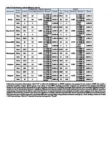
Results of hypothesis tests comparing bagging and seven active learning method accuracies to random sampling at the final training set size. ‘+’ indicates statistically significant improvement and ‘-’ indicates statistically significant deterioration. ‘NA’ indicates ‘not applicable.’ Figures 5.2-5.5 display the actual means used for hypothesis testing as solid diamonds in the box plots. . . . . . . . . . . . . . . . xii
61
5.4
Results comparing random sampling, bagging, and seven active learning methods reported as the percentage of random examples over (or under) the final training set size needed to give similar accuracies. Active learning methods were seeded with 20 random examples, and stopped when training set sizes reached final tested size (300 observations with exceptions; see Section 5.4 for details on the rationale for different stopping points). . . . . . . . . . . . . . . . . . . . . . . . .
62
5.5
The structure of the NewsGroups data set. . . . . . . . . . . . . . . .
64
5.6
Counts of different categories picked after using margin sampling on the NewsGroups data set. . . . . . . . . . . . . . . . . . . . . . . . .
5.7
69
The average percentage of matching test set margins when comparing models trained on data sets of size 300 to a model trained on the pool. Ten repetitions of the experiment produce the averages below. . . . .
6.1
70
Results of hypothesis tests comparing bagging and four active learning method accuracies to random sampling at training set size 600. ‘+’ indicates statistically significant improvement and ‘-’ indicates statistically significant deterioration. ‘NA’ indicates ‘not applicable.’ Figures 6.1- 6.2 display the actual means used for hypothesis testing. . .
6.2
73
Results of hypothesis tests comparing four heuristic active learning method accuracies to random sampling at the final training set size. These active learners used the larger candidate size of 300. ‘+’ indicates statistically significant improvement and ‘-’ indicates statistically significant deterioration compared to random sampling. ‘NA’ indicates ‘not applicable.’ Figures 6.3-6.6 display the actual means used for hypothesis testing. . . . . . . . . . . . . . . . . . . . . . . . . xiii
79
6.3
Results of hypothesis tests comparing bagging and two query by bagging methods using a bag size of 15. ‘+’ indicates statistically significant improvement and ‘-’ indicates statistically significant deterioration. ‘NA’ indicates ‘not applicable.’ Figures 6.7-6.10 display the actual means used for hypothesis testing. . . . . . . . . . . . . . . . .
xiv
80
List of Figures 2.1
Learning curve plotting classification accuracy against size of training set. The red points forming a horizontal line represent the accuracy from training on the entire pool of data. . . . . . . . . . . . . . . . .
25
3.1
Plot of the logistic function for different values of θ. . . . . . . . . . .
28
5.1
Clusters of topics based on distance measured on confusion matrix rows. The confusion matrix was computed in this case after training on the entire pool and averaging over 10 pool/test splits. . . . . . . .
5.2
53
Box plots and learning curves for Art, ArtNoisy and ArtConf data sets. Box plots show the distribution of the accuracy at the training set stopping point, with a black diamond indicating the mean. In the learning curves, random performance is drawn as connected points. Confidence bars indicate the variability of competing active learning schemes. . . . . . . . . . . . . . . . . . . . . . . . . . . . . . . . . . .
5.3
57
Box plots and learning curves for Comp2a, Comp2b and LetterDB data sets. Box plots show the distribution of the accuracy at the training set stopping point, with a black diamond indicating the mean. In the learning curves, random performance is drawn as connected points. Confidence bars indicate the variability of competing active learning schemes. . . . . . . . . . . . . . . . . . . . . . . . . . . . . . xv
58
5.4
Box plots and learning curves for NewsGroups, OptDigits and TIMIT data sets. Box plots show the distribution of the accuracy at the training set stopping point, with a black diamond indicating the mean. In the learning curves, random performance is drawn as connected points. Confidence bars indicate the variability of competing active learning schemes. . . . . . . . . . . . . . . . . . . . . . . . . . . . . .
5.5
59
Box plot and learning curves for the WebKB data set. The Box plot shows the distribution of the accuracy at the training set stopping point, with a black diamond indicating the mean. In the learning curve, random performance is drawn as connected points. Confidence bars indicate the variability of competing active learning schemes. . .
5.6
60
Squared error along with bootstrap estimates of bias and variance for Art, ArtNoisy, ArtConf, Comp2a, Comp2b, and LetterDB data sets at different training set sizes.
5.7
. . . . . . . . . . . . . . . . . . . . . .
65
Squared error along with bootstrap estimates of bias and variance for NewsGroups, OptDigits, TIMIT, and WebKB data sets at different training set sizes. . . . . . . . . . . . . . . . . . . . . . . . . . . . . .
6.1
66
Box plots and learning curves for LetterDB, NewsGroups, and TIMIT data sets with late starting and stopping points. Box plots show the distribution of the accuracy at the training set stopping point, with a black diamond indicating the mean. In the learning curves, random performance is drawn as connected points. Confidence bars indicate the variability of competing active learning schemes. . . . . . . . . . . xvi
74
6.2
Box plots and learning curves for the WebKB data set using late starting and stopping points. Box plots show the distribution of the accuracy at the training set stopping point, with a black diamond indicating the mean. In the learning curves, random performance is drawn as connected points. Confidence bars indicate the variability of competing active learning schemes. . . . . . . . . . . . . . . . . . .
6.3
75
Box plots and learning curves for Art, ArtNoisy and ArtConf data sets using a candidate sample size of 300. Box plots show the distribution of the accuracy at the training set stopping point, with a black diamond indicating the mean. In the learning curves, random performance is drawn as connected points. Confidence bars indicate the variability of competing active learning schemes. . . . . . . . . . .
6.4
76
Box plots and learning curves for Comp2a, Comp2b and LetterDB data sets using a candidate sample size of 300. Box plots show the distribution of the accuracy at the training set stopping point, with a black diamond indicating the mean. In the learning curves, random performance is drawn as connected points. Confidence bars indicate the variability of competing active learning schemes. . . . . . . . . . .
6.5
77
Box plots and learning curves for NewsGroups, OptDigits and TIMIT data sets using a candidate sample size of 300. Box plots show the distribution of the accuracy at the training set stopping point, with a black diamond indicating the mean. In the learning curves, random performance is drawn as connected points. Confidence bars indicate the variability of competing active learning schemes. . . . . . . . . . . xvii
78
6.6
Box plots and learning curves for the WebKB data set using a candidate sample size of 300. The Box plot shows the distribution of the accuracy at the training set stopping point, with a black diamond indicating the mean. In the learning curves plots, random performance is drawn as connected points. Confidence bars indicate the variability of competing active learning schemes. . . . . . . . . . . . . . . . . . .
6.7
79
Box plots and learning curves for Art, ArtNoisy, and ArtConf data sets using bag size 15. The Box plots show the distribution of the accuracy at the training set stopping point, with a black diamond indicating the mean. In the learning curves, random performance is drawn as connected points. Confidence bars indicate the variability of competing active learning schemes. . . . . . . . . . . . . . . . . . .
6.8
81
Box plots and learning curves for Comp2a, Comp2b, and LetterDB data sets using bag size 15. The Box plots show the distribution of the accuracy at the training set stopping point, with a black diamond indicating the mean. In the learning curves, random performance is drawn as connected points. Confidence bars indicate the variability of competing active learning schemes. . . . . . . . . . . . . . . . . . .
6.9
82
Box plots and learning curves for NewsGroups, OptDigits, and TIMIT data sets using bag size 15. The Box plots show the distribution of the accuracy at the training set stopping point, with a black diamond indicating the mean. In the learning curves, random performance is drawn as connected points. Confidence bars indicate the variability of competing active learning schemes. . . . . . . . . . . . . . . . . . . xviii
83
6.10 Box plot and learning curves for the WebKB data set using bag size 15. The Box plot shows the distribution of the accuracy at the training set stopping point, with a black diamond indicating the mean. In the learning curve plot, random performance is drawn as connected points. Confidence bars indicate the variability of competing active learning schemes.
. . . . . . . . . . . . . . . . . . . . . . . . . . . .
xix
84
Chapter 1 Introduction Procurement of labeled training data is the seminal step of training a supervised machine learning algorithm. A recent trend in machine learning has focused on poolbased settings where unlabeled data is inexpensive and available in large supply, but the labeling task is expensive. Pool-based active learning methods attempt to reduce the “cost” of learning in a pool-based setting by using a learning algorithm trained on the existing data and selecting the portion of the remaining data with the greatest expected benefit. In classification settings benefit may be measured in terms of the generalization accuracy (or error) of the final model. The last decade has also seen increased use of the logistic regression classifier in machine learning applications, though often under different names: multinomial regression, multi-class logistic regression or the maximum entropy classifier. In this dissertation we address the question of how to best perform pool-based active learning with the logistic regression model. We view treatment of this problem as a natural first step in developing active learning solutions to the expansive set of models derived from the exponential family of distributions, of which logistic regression is a member. 1
1.1
Active Learning: a Definition
Active learning is defined as a setting where a learning agent interacts with its environment in procuring a training set, rather than passively receiving an i.i.d. sample from some underlying distribution. The term pool-based active learning is used to distinguish sampling a pre-defined pool of examples from other forms of active learning including methods that construct examples from Rn or other sets from first principles. Henceforth we will often use the term active learning to refer to pool-based active learning; since the dissertation does not treat the other forms, no confusion will arise. Furthermore, we focus almost entirely on the problem of training classifiers. The purpose of developing active learning methods is to achieve the best possible generalization error at the least cost, where cost is usually measured as a function of the number of examples labeled. Frequently we plot the tradeoff between number of examples labeled and generalization error through learning curves of the type introduced in Chapter 2. It is commonly believed that there should exist active learning methods that perform at least as well as random sampling from a pool at worst, and these methods should often outperform random sampling. This belief is given theoretical justification under very specific assumptions [27, 64], but is also occasionally contradicted by empirical evaluations.
1.2
Why Active Learning Is Hard
Active learning is hard because random sampling from the pool provides a very competitive baseline. As a rule of thumb, the generalization error rate of a machine learning algorithm decreases according to: b Etest = a + α n 2
(1.1)
where n is the training set size, and a, b and α depend on the task and learning algorithm [24, Chapter 9]. The very attractive baseline provided by random sampling from the pool is the primary challenge that active learning methods must overcome to justify their use. In order for active learning to be accepted in industrial applications it must guarantee that the performance will offset the cost of implementing a nonrandom sampling scheme and retraining the machine learning algorithm repeatedly. Particularly daunting is that active learning is most useful when applied to a new domain where there are few examples. In a new domain, we have little guarantee that heuristics that worked in the past will work again without tuning and tweaking.
1.3
A Perspective on Active Learning
The earliest research in active learning stressed counterexample requests (e.g. [2]) or query construction [14, 46]. Focus soon turned to methods applicable to pool-based active learning including the query by committee method [64] and experimental design methods based on A-optimality [14]. The above methods are motivated by theory and explicit objective functions. Empirical evaluation of such objective function approaches has been scant due to computational costs associated with these methods. Of late, there are some signs of renewed interest in objective function approaches [34]. There has been growing interest in application of active learning to real-world data sets. A trend of the last ten years [1, 3, 20, 38, 45, 51, 54, 60, 70] has been to employ heuristic methods of active learning with no explicitly defined objective function. Uncertainty sampling [45], query by committee [64]1 , and variants have proven particularly attractive because of their portability across a wide spectrum of 1
Query by Committee is a method with strong theoretical properties under limited circumstances [27, 64], but the overwhelming trend has been to apply the method in circumstances where the theory does not apply. Often the term Query by Bagging is used to describe such ad hoc applications. Chapter 2 contains further discussion.
3
machine learning algorithms. A subtrend in the field has sought to improve performance of heuristics by combining them with secondary heuristics such as: similarity weighting [51], interleaving active learning with EM [51], interleaving active learning with co-training [67], and sampling from clusters [70], among others.
1.4
Thesis
The primary contributions of this thesis are conclusions about which of the many methods of pool-based active learning are likely to perform well for logistic regression and under what conditions. There are two main components of this work that support our conclusions. First, we re-examine the theory of experimental design in the context of the logistic regression classifier. A technique for minimizing prediction variance known as A-optimality emerges. We generalize this result to apply to a wider variety of loss functions and specifically explore log loss. Second, we use our two principled loss functions along with random sampling as a baseline in evaluating the alternative heuristic methods of active learning. Ultimately, we use the evaluations to make conclusions about the performance of different active learning methods. The empirical investigations within this dissertation have several pertinent features. Our evaluations of the loss function methods are the largest scale of any to date in a pool-based active learning setting. So these evaluations are an opportunity to test the hypothesis that the computational costs of principled methods come with performance gains. Noting that heuristic methods occasionally perform worse than random, we also explore the causes of these failures, and identify conditions that lead the uncertainty sampling heuristics to failure. 4
1.5
Variance Reduction (A-Optimality) Explained
Logistic regression is a method that assigns probabilities to the class labels of observations. We choose as our first objective for active learning of logistic regression the minimization of the prediction variance: X c
VarD [ˆ π (c, x; D)] =
X c
h
i
ED (ˆ π (c, x; D) − ED [ˆ π (c, x; D)])2 ,
(1.2)
where π ˆ (c, x; D) is a logistic regression model trained on D. The model outputs the predicted probability that label c is associated with observation x. The parameter c indexes the different categories of the classification task, and the expectation ED is with respect to training sets of fixed size. More generally, we can compute the prediction variance over an entire set of examples, for instance the pool of unlabeled data. This is the same variance term that emerges from the bias/variance decomposition of mean squared error (MSE) (detailed in Chapter 4). Statistical theory governing the behavior of the members of the exponential family (logistic regression is a member) permit an asymptotically correct measurement of variance. These two essential components, the ability to measure variance, and a link between decrease of variance and decrease in mean squared error make Equation 1.2 a compelling objective function for active learning.
1.6
Applicability of Our Approach to Structured Data
Beyond the classification setting there are a variety of prediction tasks where response variables are statistically dependent. Such prediction problems include: part of speech tags [19], parse trees [17], simultaneous predictions of syntax and semantics, optical character recognition, and gesture [50], among many others. In developing 5
active learning solutions for these tasks it is natural to look first at the simpler classification setting for hints about which theories work and why. For this reason, we spend a bit of time relating logistic regression to more expressive models capable of handling prediction of discrete categories that are statistically dependent. Chapter 4 develops the theory of A-optimality and touches on applicability of the approach to more general settings. The methodology and results of diagnosing noise, squared bias and variance portions of squared error developed in the dissertation is also relevant to statistically dependent response variables. The heuristics employed for logistic regression active learning are applicable to learning in the presence of statistically dependent response variables, as well.
1.7
Dissertation Road Map
The remainder of the dissertation proceeds as follows. Chapter 2 reviews the various methods of active learning evaluated and gives some historical background. Chapter 3 introduces the logistic regression classifier, details its statistical properties and explains its relationship to other well-studied models. Chapter 4 introduces a loss function approach to active learning motivated by experimental design. Chapter 5 describes the empirical evaluation and results for all methods, while Chapter 6 examines the effects of alternative evaluation design decisions. Chapter 7 summarizes the findings of the dissertation.
6
Chapter 2 Pool-Based Active Learning for Classifiers: A Review In this chapter we introduce some of the core algorithms and concepts from poolbased active learning and experimental design. The main focus is on classification problems with noise, and on active learning methods that can be used with logistic regression. We also touch on developments for linear regression in order to introduce some of the important concepts from the field of experimental design as a whole. We omit discussion of recent developments specific to other learning algorithms, such as large margin classifiers [26, 62, 73] and Bayesian belief networks [72]. Here, we present the theory of A-optimality and give a historical perspective on where it has been derived and how it has been applied in active learning. Through extensive literature review we demonstrate that the method has not been thoroughly evaluated in pool-based active learning scenarios. In fact, we find only one known evaluation on a non-artificial data set. There have been several evaluations using artificial neural networks on artificial data, but these data sets have had only a small number of predictors. 7
Following a convention that has developed in the active learning field we divide the “classical” active learning approaches of the early to mid 1990s into “objective function” and “heuristic” (or “algorithm independent”) methods. The objective function methods include experimental design methods such as A, D, and c−optimality. The heuristic methods include uncertainty sampling and query by committee. In actuality, the line between having an explicit objective function and a heuristic can be blurred as heuristic approximations to objective functions are made for the benefit of expediency. An alternative view is that a heuristic approach is actually an objective function approach whose assumptions have not yet been exposed.
2.1
A General Purpose Active Learning Framework
Algorithm 1 A Generalized Active Learning Loop Require: partial training set, pool of unlabeled examples repeat Select T random examples from pool Rank T examples according to active learning rule Present the top-ranked example to oracle for labeling Augment the training set with the new observation until Training set reaches desirable size
Different approaches to active learning amount to different methods of assessing the value of labeling individual examples. All pool-based active learning methods fit into a common framework described by Algorithm 1. The key difference between active learning methods is the method for ranking the candidate observations for labeling. The framework is wide open to the type of ranking rule employed. Usually, the ranking rule incorporates the model trained on the currently labeled data. This is the reason for the requirement of a partial training set when the algorithm begins. 8
Other active learning researchers use variants of Algorithm 1. For example, some label the top n examples in addition to the top example in order to decrease the number times a learner is retrained. Other researchers mix active learning with random labels. This dissertation will focus on labeling one example at a time. In principle this gives a rigorous method the opportunity to pick only the best examples.
2.2
Objective Function Approaches
Objective function active learning methods such as D, c, and A-optimality explicitly quantify the differences between an ideal classifier and the currently learned model in terms of a loss or other type of objective function. Borrowing notation from Roy and McCallum [60] for the special case where the learning algorithm outputs a probability distribution, a representation of an objective function follows: Z
L(π(y|x), π ˆD (y|x))P(x),
(2.1)
x,y
where L is a loss function, π(y|x) are the probabilities associated with a model trained on the entire pool, and π ˆD (y|x) are the probabilities of a model trained on a partial representation of the pool where observations (x, y) follow training set distribution D. P(x) is the distribution governing predictor variables estimated using the pool, which is presumably quite large. Example loss functions for Equation 2.1 include log loss and squared loss. In many settings a model outputs something other than a probability, such as a real value, in which case the notation needs altering: Z
ˆ L(f (x; w), f (x; w))P(x)
x
ˆ are parameters analogous to π and π where w and w ˆ. 9
(2.2)
2.2.1
A-Optimality for Linear Regression Models
To maintain chronological accuracy and develop the requisite algebraic methodology, we start with the classic design criteria of linear regression [25], with the familiar model of the data given by a Gaussian with an isotropic noise model: y|w,σ2 ∼ N (w′ X, σ 2 I).
(2.3)
The vector y encodes a set of real values. X is the design matrix, and its rows consist of the predictors of the model. The vector w is the parameter vector of the model. The maximum likelihood solution is equivalent to the least squares solution: X
arg min w
n
(yn − w · xn )2
(2.4)
ˆ = (X ′ X)−1 X ′ y. w
(2.5)
The matrix X ′ X is the observed Fisher information matrix of the linear regression. The model is frequently regularized by adding a penalty according to the magnitude of ||w||2 : arg min w
X n
(yn − w · xn )2 +
ˆ = (X ′ X + w
1 ||w||2 2 2σp
(2.6)
1 −1 ′ I) X y σp2
(2.7)
in which case the Fisher information matrix becomes: (X ′ X + σ12 I). The regularized p
variant is equivalent to a Bayesian linear regression where Equation 2.3 is augmented with the assumption: w ∼ N (0, σp2 I),
(2.8)
where the p in σp stands for “prior” to draw attention to the fact that it is a different parameter from the error variance σ 2 of Equation 2.3. Having defined the model of interest, linear regression, we contemplate now what objective function will obtain good prediction accuracy. A large portion of the experimental design literature has focused on two types of experimental goals: extremum 10
performance and model identification problems. This dissertation is concerned with the quality of predictions over the pool where the pool is taken as an accurate representation of the distribution of a final test set. Therefore we focus on an extremum problem: minimizing an expected loss computed over the pool. The common choice of loss for real-valued regression modeling is expected squared error, which decomposes into portions that represent pure noise (or model misspecification) and loss due to small training set size: E[(y − f (x; D))2 |x, D] = E[(y − E[y|x])2 |x, D] “Noise” + (f (x; D) − E[y|x])2 .
(2.9) (2.10)
The E above is an expectation with respect to the probability distribution generating observations (x, y). The term E[y|x] represents the expectation of y given x according to the true distribution generating (x, y). The variable D represents a training set. The second term is highly dependent on the training set while the first term is independent due to conditioning. The mean squared error (MSE) of f is the expectation of the second term with respect to training sets D of fixed size s: EDs [(f (x; D) − E[y|x])2 ].
(2.11)
The variable s is frequently omitted in the literature, a convention we will adopt. MSE is difficult to measure; even if we could compute ED we do not have access to E[y|x]. Fortunately, mean squared error may be decomposed into bias and variance portions of error which are both somewhat easier to estimate: ED [(f (x; D) − E[y|x])2 ] = (ED [f (x; D)] − E[y|x])2 “bias squared”
(2.12)
+ED [(f (x; D) − ED [f (x; D)])2 ]. “variance” [33] provides more details on these identities. The variance term describes the tendency of regressors to vary with respect to an input distribution of fixed size. The 11
bias term captures the difference between the expected model output and the actual expected value of y given x. We will explore these concepts in greater depth in chapter 4. For linear regression, an experimental design objective function often used to obtain good prediction accuracy is the variance component of MSE: Var[f (x; D)] = ED [(f (x; D) − ED f (x; D))2 ].
(2.13)
There are two reasons for the popularity of this technique. The first is that it is evident from the decomposition (2.12) that decreasing variance will lead to decreased MSE. The second reason is that statistical theory allows efficient estimation of variance. Some needed facts in deriving an optimality criteria from this objective function ˆ be the maximum likelihood (and therefore least squares) paramfollow. First, let w ˆ ∼ N (w, F −1 ), where w, w ˆ are both vectors, F is eters for linear regression. Then w
ˆ ′ x) = xF −1 x as a consequence of northe Fisher information matrix [63], and Var(w ˆ With this result in hand, we derive the prediction variance incurred by mality of w. making predictions over the pool of unlabeled data. Define An = xn x′n , A = and compute: X
ˆ = Var(x′n w)
n∈Pool
X
xn F −1 xn by Normality
X
tr xn x′n F −1
X
tr An F −1
P
n
An
(2.14)
n∈Pool
=
n∈Pool
=
n∈Pool
n
n
n
o
= tr AF −1 .
o
o
(2.15) (2.16) (2.17)
Equation 2.17 is referred to as A-optimality due to the A matrix that gives the method its name. Equation 2.14 is referred to as c-optimality; when the vectors xn are renamed cn the naming becomes more apparent. Before moving on, we give a formal definition of the Fisher information matrix 12
computed over a likelihood function f : ∂ 2 ln f (X|θ) = −E . ∂θi ∂θj "
I(θ)ij
#
(2.18)
For expediency, we will frequently denote the matrix I(θ) as F , making implicit the dependence on the parameters θ.
2.2.2
D-Optimality for Linear Regression Models
Imagine the goal of training a statistical model is the model itself rather than the application of the model. For instance, the slope in a simple linear regression can represent the dependence of a reaction rate on the abundance of substrate. Learning the slope parameter accurately gives insight into a natural phenomenon. D-optimality concerns the model identification objective of designing experiments. Though our focus in this dissertation with classification accuracy leads to prediction accuracy rather than model identification as our primary focus, the reader will benefit from knowledge of this very popular experimental design criterion in placing the current active learning approaches in context. It is virtually impossible to find introductions to statistical experimental design without references to D-optimality, and so it will be helpful to understand the method. Furthermore, there are applications of active learning objective functions that follow in the spirit of D-optimality [72] so having a definition of D-optimality will help identify this trend and note its difference from the A-optimality “prediction variance” approach. ˆ of a linear regression follow a normal Since the maximum likelihood parameters w ˆ ∼ N (w, F −1 ) [63], we may write out the distribution over parameters: distribution w ˆ P(w|w, X, σp2 )
=
µ
1 2π
¶d/2
1
1 q ˆ − w)′ F (w ˆ − w) exp − (w −1 2 |F | ½
¾
(2.19)
From the Gaussian above we see that a measure of parameter variance is given by the determinant: |F |. In geometric terms, this is the inverse of the volume of the parallelepiped encoded by the rows of the Fisher information matrix. Maximizing 13
this determinant gives the D-optimality criterion. The D in the name D-optimality comes from “determinant.” In the Bayesian setting, we may derive the D-optimality criterion through the Shannon information measure of model uncertainty: Z
P(y, w|X) log
P(w|y, X) dw dy. P(w)
(2.20)
Noting that P(w) does not depend on the design X, we may reexpress the objective function in a more streamlined form: Z
P(y, w|X) log P(w|y, X) dw dy.
(2.21)
Our goal is to maximize the expected information gain from the experiment, which is equivalent to maximizing the Kullback-Leibler (KL) divergence between the prior and posterior models. Applied to linear regression, Equation 2.21 becomes [12]: n o k 1 k − log(2π) − + log det σ −2 F , 2 2 2
(2.22)
and once again we find that maximizing |F | is the optimal solution. As a byproduct of these derivations, we see that maximizing the expected information gain on the linear regression parameters is equivalent to minimizing model uncertainty. In both D- and A-optimality for linear regression, selecting examples is independent of the response values y, a fact exploited by Schein et al. [61] for selecting a training set before any labeling at all has occurred. In nonlinear models, we are not so lucky; the Fisher information depends on the response of the design matrix.
2.2.3
A-Optimality for Nonlinear Regression Models
A-optimality can be extended to a wide range of non-linear regression models; a template is given in [12]. In Chapter 4 we derive a method for logistic regression. For now we explore the special case of backpropagation neural networks (BPNN) where the method has been applied in the past. In his Ph.D. dissertation [46] 14
and companion publications [48, 47], MacKay derives the A-optimality and similar information-based objective functions for active learning of backpropagation neural networks inside a Bayesian setting. It was Cohn [14] who first evaluated A-optimality for backpropagation neural networks on “natural” data. Neural networks may be trained using a variety of loss functions. Our discussion of backpropagation neural networks will consist solely of those networks fit with the least squares objective function, with its implicit Gaussian likelihood interpretation, i.e. we find parameter vector w that minimizes [7]: X n
(f (xn ; w, A) − tn )2 +
1 X 2 w σp2 d d
(2.23)
where tn is the observed training set output for observation n, and the second term in the summation provides model shrinkage as in the linear case. From this point we ignore the parameter A specifying the network architecture, and assume the architecture is fixed. The objective function to be minimized through active data selection is again the variance: X
n∈Pool
Var[f (xn ; D)] =
X
n∈Pool
ED [(f (xn ; D) − ED f (xn ; D))2 ].
(2.24)
The derivation of A-optimality for back-propagation neural networks follows in the spirit of the logistic regression derivations described in Chapter 4. Key differences exist between employing the method for logistic regression and backpropagation neural networks, at least when comparing the implementations of this dissertation to the previous implementations for backpropagation neural networks. Neural networks suffer from local minima in the training surface whereas logistic regression has a global maximum. The issue is relevant when retraining the models quickly using previously estimated parameters as seeds. The Fisher information matrix of 2.23 is frequently approximated in the neural network literature (e.g.
[14]), whereas our
evaluations will employ the actual Fisher information matrix for logistic regression. A-optimality for BPNN was evaluated on natural data by Cohn [14] who trained a neural network with 2 inputs, a single layer of 20 hidden units, and 2 outputs 15
for a grand total of 80 parameters encoded in vector w. Hidden and output units were sigmoid, trained with the backpropagation procedure which minimizes squared error. The method was evaluated by selecting up to 100 observations. Despite an extensive search of the literature through document databases such as Researchindex, we could not find any other evaluation of nonlinear regression variance reduction active learning on natural data in a pool-based active learning setting. This is surprising given that Cohn’s 1996 paper [14] and its earlier incarnation [13] are very well cited. Personal communication with Dr. Cohn, however, substantiates this assertion [16]. We were able to find some evaluations of variance reduction active learning on artificial data [31, 69]. The examples that include noise in the data generation process use a homoscedastic noise generator, in contrast to real data which often contain heteroscedastic noise. The number of input units in these evaluations never exceed 4 and the number of hidden layer units never exceed 7. A single output unit was used in these evaluations. The largest number of parameters ever employed in an evaluation on artificial data that we could find was 35, and the evaluation was by Fukumizu [31]. Because of the larger size and different noise structure of real data, there is no guarantee that the simulated data results above will hold for natural data.
2.2.4
An Information Theoretic Variant of A-Optimality
The derivation of A-optimality suggests a closely related information theoretic objective function [46, 48]. The intuition is the following. Since the A-optimality criterion is derived by adding up the variance terms of individual Gaussians that result from predictions over the pool, why not use instead the entropy of those individual Gaussians and add them up? Let S(P(yn )) denote the entropy from the prediction on 16
observation n. The resulting objective function is: S =
X
S(P(yn ))
(2.25)
n
=
1X log(c′n F −1 cn ) + constant 2 n
(2.26)
This quantity differs from A-optimality, since entropy is a nonlinear function of the variance term (c′n F −1 cn ). This is not the first information theory criterion we have seen: recall the information theoretic definition of D-optimality in Section 2.2.2. Variants of Equation 2.26 have been applied in experimental design as well, and are reviewed in [12].
2.2.5
Bias and Mean Squared Error Minimization
In addition to variance-minimization techniques such as A-optimality, researchers have attempted to minimize other portions of the error decomposition of Equation 2.12. Cohn [15] explores minimization of the bias squared portion of error for locally weighted regression models using techniques such as fitting a higher order polynomial and measuring the difference, residual bootstrapping, and fitting the model’s own cross-validated residuals. Sugiyama and Ogawa [68] minimize both bias and variance through a two-stage sampling approach. Both methods look promising, but empirical evaluation across diverse natural data sets is still lacking. Through our own evaluations, we will gain a sense of how much improvement is gleaned from variance minimization of logistic regression. This should help assess the need to develop solutions for other portions of mean squared error.
2.3
Algorithm Independent Approaches
We now turn to algorithm-independent approaches to active learning such as uncertainty sampling and query by committee. In the general classification setting that 17
this dissertation focuses on, little can be said that relates these approaches to explicit objective functions. Under a few assumptions, including at a minimum the assumption that classification is a noise free function of the predictors, it may be possible to establish a relationship between each of these methods and an objective function. The lack of principled motivation for these heuristic methods in more general settings has not stopped the empirical machine learning community from evaluating the methods on actual data sets [1, 3, 20, 38, 45, 51, 54, 60, 70, 71]. In fact, by looking at the literature that has amassed around the heuristic methods, one gains a sense of optimism for active learning as a whole. Our own experience with these methods paints a less rosy picture; the methods frequently produce results that are worse than random sampling from the pool. Traces of these negative results can be found within the empirical evaluations cited, but we wonder whether the literature as a whole might be biased towards positive results. In our evaluations we look at three types of heuristics for active learning: uncertainty sampling, query by committee and classifier certainty. We describe these methods along with their computational complexities, and then briefly review variations of these methods in the remaining subsections.
2.3.1
Uncertainty Sampling
Uncertainty sampling is a term invented by Lewis and Gale [45], though the ideas can be traced back to the query methods of Hwang et al. [39] and Baum [4]. We discuss the Lewis and Gale variant since it is widely implemented and general to probabilistic classifiers such as logistic regression. The uncertainty sampling heuristic chooses for labeling the example for which the model’s current predictions are least certain. The intuitive justification for this approach is that regions where the model is uncertain indicate a decision boundary, and clarifying the position of decision boundaries is the goal of learning classifiers. 18
A key question is how to measure uncertainty. Different methods of measuring uncertainty will lead to different variants of uncertainty sampling. We will look at two such measures. As a convenient notation we use q to represent the trained model’s predictions, with qc equal to the predicted probability of class c. One method is to pick the example who’s prediction vector q displays the greatest Shannon entropy: −
X
qc log qc .
(2.27)
c
Such a rule means ranking candidate examples in Algorithm 1 by Equation 2.27. An alternative method picks the example with the smallest margin: the difference between the largest two values in the vector q. In other words, if c, c′ are the two most likely categories for observation xn , the margin is measured as follows: ˆ ˆ ′ Mn = |P(c|x n ) − P(c |xn )|.
(2.28)
In this case Algorithm 1, would rank examples by increasing values of margin, with the smallest value at the top of the ranking. The original definition of uncertainty sampling [45] describes the method in the binary classification setting, where the two definitions of uncertainty are equivalent. We are not aware of previous usages of minimum margin sampling active learning in multiple category settings except when motivated as a variant of query by committee (see Section 2.3.2). Using uncertainty sampling, the computational cost of picking an example from T candidates is: O(T DK) where D is the number of predictors, K is the number of categories. In the evaluations we refer to the different uncertainty methods as entropy and margin sampling.
2.3.2
Query by Committee
Query by committee (QBC) was proposed by Seung, Opper and Sompolinksy [64], and then rejustified for the perceptron case by Freund et al. [27]. The method assumes: 19
• A noise-free (e.g. separable) classification task. • A binary classifier with a Gibbs training [65] procedure. Under these assumptions and a few others [27, 64] a procedure can be found that guarantees exponential decay in the generalization error: Eg ∼ e−nI(∞)
(2.29)
where I(∞) denotes a limiting (in committee size) information gain and n is the size of the training set. Compare Equation 2.29 to 1.1, to see the advantages of the method. A description of the query by committee algorithm follows. A committee of k models Mi are sampled from the version space over the existing training set using a Gibbs training procedure. The next training example is picked to minimize the entropy of the distribution over the model parameter posteriors. In the case of perceptron learning, this is achieved by selecting query points of prediction disagreement. The method is repeated until enough training examples are found to reduce error to an acceptable level. Alas, the assumptions of the method are frequently broken, and in particular the noise-free assumption does not apply to logistic regression on the data sets we intend to use in the evaluations. The noise-free assumption is critical to QBC, since the method depends on an ability to permanently discard a portion of version space (the volume the parameters may occupy) with each query. Version space volume in the noisy case is analogous to the D-optimality score, since a determinant is essentially a volume measure. Generally the model variance, as measured through the Doptimality score of linear and non-linear models, does not decrease exponentially in the training set size even under optimal conditions. The use of the query by committee method in situations where the assumptions do not apply is an increasing trend with the modifications of Abe and Mamitsuka [1] and McCallum and Nigam [51] who substitute bagging for the Gibbs training procedure. 20
The term “query by bagging” (QBB) is becoming a catchphrase for algorithms that take a bagging approach to implementing the query by committee procedure. Query by bagging is implemented as follows. An ensemble of models fˆi is formed from the existing training set using the bagging procedure [9]. An observation is picked from the pool that maximizes disagreement among the ensemble members. The procedure is repeated until enough training examples are chosen. As a modification to Algorithm 1, the following lines replace the original line that produces a ranking. The general purpose active learning loop of Algorithm 1, is augmented as follows: Use bagging [9] to train B classifiers fˆi Rank candidates by disagreement among the fˆi The definition of disagreement is wide open and several methods have been proposed. A margin-based disagreement method is to average the predictions of the fˆi (normalizing to ensure a proper distribution), and using the margin computation of Equation 2.28. We refer to this method as QBB-AM [1] (query by bagging followed by author’s initials). An alternative approach to measuring disagreement is to take the average prediction (as above) and measure the average KL divergence from the average: B 1 X KL(fˆb ||fˆavg ) B b=1
(2.30)
Larger values of average divergence indicate more disagreement, and so ranking occurs from larger to smaller values in Algorithm 1. Following the convention of using the author’s initials, we refer to this method as QBB-MN [51]. Under these two disagreement measures, query by bagging methods take only slightly more computational time than certainty sampling methods: O(BT DK); the cause of the difference is inclusion of the bag size B in the formula. 21
2.3.3
Classifier Certainty
For logistic regression and other probabilistic classifiers, several researchers have proposed minimizing the entropy of the algorithm’s predictions [46, 47, 60]1 :
CC = −
X
p∈Pool
X
ˆ ˆ P(c|x p ) log P(c|xp )
(2.31)
c
as a criteria for picking a training set. The sum is over the pool of unlabeled data and the set of categories. In intuitive terms Equation 2.31 measures degree of certainty of the individual classifications over the pool, and so we call the method the Classifier Certainty (CC) method. In order to rank examples in Algorithm 1, an expected ˆ foreach candidate. The value of CC is computed with respect to the current model P expectation is over possible labelings of the candidate. A more detailed explanation of the expectation procedure is given in Section 4.3 of Chapter 4. Note however, that CC is not a proper loss function and minimization need not lead to good accuracy; Equation 2.31 does not depend on the true probabilities P but ˆ For example, we often find ourselves certain of facts or beliefs only the estimates P. that are later found not be true. Restricting the search for examples to those that makes us more certain of previously held beliefs can be a bad choice when learning. Excluding the cost of model fitting, implementation of CC is at worst: O(T N KD), where N is the number of observations from the pool used to compute the benefit of adding an observation, D is the number of predictors, T is the number of candidates evaluated for labeling, and K is the number of categories. An approximation that saves computational time is Monte Carlo sampling from the pool to assess the benefit of labeling. For example, in our evaluations, we sample 300 examples from the pool to assess model improvement. 1
Some readers familiar with the language modeling literature will be used to “prediction entropy” as a measure of performance. However, in language modeling, it is actually a cross-entropy that is measured, not prediction entropy for the reasons outlined below.
22
2.3.4
Heuristic Generalizations and Variations
Uncertainty sampling and query by committee methods appear so general in their implementation that it is tempting to port the methods to more complex problems than the classification setting. Such has happened in the case of part of speech tagging, where the query by committee methods are generalized to apply to hidden Markov models [20]. In parsing, uncertainty sampling [38] and other heuristic approaches have been applied [70]. A recent trend in the pool-based active learning literature has been to take various approaches, usually uncertainty sampling or query by committee and try to improve performance through additional heuristics. Such schemes include: observation similarity weighting [51], sampling from clusters [70], interleaving labeling with EM [51], interleaving labeling with co-training [67], increasing diversity of ensembles [54], among others. These sorts of variations are so numerous that we are unable to evaluate them here.
2.4
Challenges: Model Misspecification and Broken I.I.D. Assumptions
Model misspecification is the phenomenon where the data do not fit the assumptions of the model. An example of misspecification is when the data are generated by a neural network with many hidden units, but the model employed is linear. Objective function methods, including the experimental design methods, are derived implicitly assuming that the response variable is generated by the model. How much misspecification may hurt the various active learning methods is unknown. MacKay [46] and Cohn [14] have both looked at this question on specific data sets. We explore this question in evaluations by controlling the noise level of the data sets. Yue and Hickernall [74] tackled misspecification for linear regression models; this is the only 23
work we know of that has focused on correcting the problem. A separate problem with active learning methods is that most of the theory of objective function approaches and intuitions of heuristic approaches rely on i.i.d. assumptions of the training set. In the nonlinear A-optimality case, one particular area of concern is the asymptotic approximation to variance, which relies on an i.i.d. assumption. A proper specification of the problem and its consequences are an interesting challenge.
2.5
Active Learning Evaluation Methodology
The largest evaluations of active learning have been conducted using decision trees and variants of query by committee [1, 54] on UCI machine learning repository data [8]. Document classification [51] and other natural language processing domains are areas under frequent investigation [3, 20, 38, 70]. Evaluations typically try to show increased performance relative to the random baseline. Proof of enhanced performance can take the form of showing how many more examples are necessary to obtain a certain performance or demonstrating superior performance at a fixed training set size. Learning curves such as Figure 2.1 demonstrate performance for different training set sizes, but have the disadvantage of taking up so much space that comparing across different data sets using multiple competing methods can be cumbersome. An alternative approach of reporting results is tabular form where results are reported after training on some fixed number of observations, such as 300. There are several variables of an evaluation that must be decided. How many random examples do we assume are labeled before active learning will begin? Should we use use a purely active learning approach to sampling (as performed in [51, 60]) or mix active learning with random sampling (e.g.
[3]). Also, some evaluations
choose to sample more than one point at a time before re-training for computational 24
"LetterDB Data Set" 0.8
Entire Pool Random Sampling
Classification Accuracy
0.7
0.6
0.5
0.4
0.3
0.2 0
50
100
150 Training Set Size
200
250
300
Figure 2.1: Learning curve plotting classification accuracy against size of training set. The red points forming a horizontal line represent the accuracy from training on the entire pool of data.
25
expediency [54]. Our experience is that different choices for each of these variables may lead to different conclusions about performance and robustness of a method. One of our goals is to isolate the effects of different decisions. Chapter 6 focuses on this issue.
2.6
Summary
This chapter gave a tour of active learning serving the purposes of conveying a sense of the breadth of previously developed methods while spelling out the details of particular methods we will evaluate in Chapters 5 and 6. We maintained a degree of chronological accuracy; the experimental design methods were proposed as a method for active learning before most of the heuristic methods, and well before the heuristic methods caught on. Experimental design now seems to be unknown to much of the machine learning community due to the recent emphasis on heuristic methods and the recent entry of most members of the active learning community. It has been unknown until now how well experimental design methods work on naturally occurring data.
26
Chapter 3 The Logistic Regression Classifier In this chapter, we introduce the logistic regression classifier and state its mathematical and statistical properties. We present the logistic regression model as the intersection of various diverse frameworks including: generalized linear models, maximum entropy classifiers, the exponential family of distributions, and the conditional random field model. We detail both the commonalities and the distinctions between logistic regression and these other frameworks. Understanding the place of logistic regression in the scheme of other widely used models will prove useful to those who would like to explore the active learning techniques of this dissertation in wider contexts.
3.1
Logistic Regression: A Bernoulli Probability Model
In describing logistic regression [37], we begin with a definition of the logistic function: σ(θ) =
1 . 1 + exp[−θ] 27
(3.1)
1 0.8
σ(θ)
0.6 0.4 0.2 0 −4
−3
−2
−1
0
θ
1
2
3
4
Figure 3.1: Plot of the logistic function for different values of θ.
The logistic function is a continuous increasing function mapping θ into the interval (0, 1). Figure 3.1 illustrates the logistic function mappings for a range of input values. We can see that at θ = 0, σ(θ) = 0.5. As θ increases the function output approaches 1, and as θ decreases (e.g. larger in magnitude, yet negative), the output approaches 0. Therefore, the function is suitable for representing the probability of a Bernoulli trial outcome. Given a set of predictors, xn , we wish to determine the probability of a binary outcome yn . We define a probability model: . P(Yn = 1|xn ) = σ(w · xn )
(3.2)
with corresponding likelihood function: P(y|xn , n = 1 . . . N ) =
Y n
=
Y n
σ(w · xn )yn (1 − σ(w · xn ))(1−yn )
(3.3)
σ(w · xn )yn σ(−w · xn )(1−yn ) .
(3.4)
Equation 3.3 has a Bernoulli distribution form. A useful variant for scientific and sociology experiments employs a binomial [6] rather than Bernoulli formulation to facilitate repeated trials. 28
3.2
Multinomial Probability Model
When the number of outcome categories exceeds two, the situation is a little more complex; the outcome variables Yn take on one of three or more discrete outcomes rather than a 0 or a 1. We define a probability model as follows: exp(wc · xn ) . P(Yn = c|xn ) = π(c, xn , w) = P . c′ exp(wc′ · xn )
(3.5)
The parameter vector w of the binary logistic model is augmented by a set of vectors wc : one for each category. The resulting likelihood is: P(y|xn , n = 1 . . . N ) =
Y
π(c, xn , w)ync .
(3.6)
nc
The multinomial model is a generalization of the binary case as can be seen by defining w0 = 0 and w1 = w in which case: exp(w · xn ) exp(0 · xn ) + exp(w · xn ) exp(w · xn ) = 1 + exp(w · xn ) 1 = 1 + exp(−w · xn ) = σ(w · xn ).
P(Yn = 1|xn ) =
3.3
(3.7) (3.8) (3.9) (3.10)
Relationship to the Exponential Family of Distributions
A distribution is a member of the exponential family if it may be written [6]: P(x; θ) = h(x) exp[
k X
j=1
ηj (θ)Tj (x) − B(θ)],
(3.11)
where θ is a vector of parameters, x is an observation, and Tj (x) are real-valued functions [6]. The logistic regression model may be written in this way by partitioning the parameters into blocks using an index over categories: η(θ)cj (encoding 29
parameters for category c, predictor j), and rewriting the function as a conditional probability: k X
P(Yn = c|xn ; θ) = h(x) exp[
j
η(θ)cj Tcj (ync ) − B(θ)]
(3.12)
and defining: θcj = wcj where w comes from (3.5) η(θ)cj = wcj xj 1
Tcj (y) =
(3.14) if y = c
(3.15)
0 otherwise
B(θ) = log
X c′
h(x) = 1.
(3.13)
exp(η(θ)c′ · x)
(3.16) (3.17)
The use of the predictors x in the function B requires some very mild restrictions on the distribution being modeled in order for (3.12-3.17) to be considered a member of the exponential family (see [6, Section 6.5] for details).
3.4
Relationship to Generalized Linear Models
Generalized linear models [53] are probability models that can be factored into an exponential family form: P(Y = y; X = x, η) = exp[ηy − A(η)]h(y) where
(3.18)
η = h(x, w)
(3.19)
The function h(·, ·) factors the model into a different set of parameters w. The appropriate choice of the functions h(·, ·) and h(·) reproduces logistic regression: h(x, w) = w · x
(3.20)
h(y) = 1
(3.21)
A(η) = log(1 + exp(w · x)).
(3.22)
30
The case where the number of categories exceeds two can be factored into a multi parameter exponential family with h function of the form of 3.19. A more formal exposition of the generalized linear model exposition is given in [6, 53]. The key advantage of viewing models this way is the ability to substitute different choices of h within a common framework. Standard choices exist for Bernoulli (e.g. logistic regression), Poisson, normal, and gamma distributions among others. In the normal case, standard linear regression emerges.
3.5
Relationship to Maximum Entropy Classifiers
Another way to parameterize a classification probability is: exp[ i λi fi (x, c)] . P(Y = c|x) = P P ′ c′ exp[ i λi fi (x, c )] P
(3.23)
The functions f are referred to as feature functions. Solving for the parameters λ using maximum likelihood techniques unveils the maximum entropy model which is frequently used in natural language processing tasks [5, 59, 57]. Usually the classifier is motivated by a desire to make the prediction probabilities highly entropic subject to constraints of matching empirical qualities of the training set (see [5]). Such motivation is the source of the name “maximum entropy model.” For our purposes, maximum entropy motivations are distracting and we [35] view the model as a mere parameterization of the distribution over categories. Logistic regression may be encoded within the maximum entropy model as follows: λcj = wcj ′
(3.24)
xnj
fcj (xn , c ) =
0
when c′ = c
(3.25)
otherwise
The parameters λ and feature functions f doubly index in the new formulation. 31
Putting these pieces together we have: exp[ ci λci fci (x, y)] P(Y = y|x) = P P ′ c′ exp[ ci λci fci (x, c )] exp[wy · x] = P . c′ exp[wc′ · x] P
(3.26) (3.27)
In contrast, there are maximum entropy distributions that cannot be represented with a logistic regression model. For instance, consider the following three-category (a, b, c) model with feature function fm in addition to features taking the form of Equation 3.25. Feature function fm is defined as follows: xnj
fm (xn , c) =
when yn = a or b
0
.
(3.28)
otherwise
The parameter λj is active in the numerator for P(Y = a|x) and P(Y = b|x). The logistic regression parameterization (3.5) does not permit such tying together of parameters to multiple categories. The vast majority of published accounts of the maximum entropy classifier do not use such non-trivial features as Equation 3.28, and it is safe to refer to such applications of the model as logistic regression. In the binary classification setting, such pathologies involving special parameters do not occur; parameters tied to both categories in binary settings can be factored away from both numerator and denominator of Equation 3.5. Thus, maximum entropy classifiers for binary tasks can always be encoded in logistic regression.
3.6
Relationship to Conditional Random Field Models
Markov random field (MRF) models (see [28, 42] for tutorials) define a probability distribution while representing the statistical dependency structure using a graph, denoted G. The nodes on the graph represent variables X i . We use the superscript notation to bring attention to the fact that the is refer to different variables, whereas 32
subscripts refer to indices for separate observations. An MRF defines a local Markov property: n
o
P(X i = xi |X \ X i ) = P(X i = xi |ni ).
(3.29)
Equation 3.29 says that the probability distribution governing X i conditioned all other variables with the exception of X i is equal to the distribution of X i conditioned on its neighbors (denoted ni ). As long as the joint distribution over X is strictly positive, the distribution may be factored into the cliques qi of G [36]: P(X = x) =
exp
³P
qj ∈G
´
φ(qj ))
Z(x)
.
(3.30)
The functions φ are called clique potentials, while the function Z is a normalizing constant ensuring x P(x) dx = 1. R
The problem of modeling the the joint distribution of variables Y given a set of variables X, where Y and X are a partition of the original set of variables of Equation 3.30, is similarly decomposed according to the Hammersley-Clifford theorem [36]: P(Y = y|X = x) =
exp(
φq (y, x)) Z(C(Y))
P
q∈C(Y )
(3.31)
where C(Y) denotes the cliques that include graph vertices Y . Lafferty et al. [44] propose a conditional random field model as a general framework for more directly modeling the variables of interest (the Y) rather than modeling both X and Y as is usually the case using hidden Markov models and Bayesian belief networks. Tasks where the conditional model has been used to replace joint models include: sequence models for part of speech tagging [44], NP chunking [66], and information extraction [43] among others, and the list is growing rapidly. When the graph C is a tree, the conditional distribution may be re-written: P(y|x) =
exp[
P
e∈E,k
λk fk (e, y|e , x) + v∈V,j µj gj (v, y|v , x)] Z(µ, λ, x) P
33
(3.32)
which is the presentation of Lafferty et al. [44]. The variables E and V continue to denote the edges and vertices of a graph, µ and λ are parameter vectors, and the notation y|s are components of the graph y with vertices in subgraph s. Equation 3.32 can be refactored [66]: P(y|x) =
exp[λ · F (y, x)] Zλ (x)
(3.33)
taking on a form quite similar to the maximum entropy model (Equation 3.23). It is evident from the forms of Equations 3.32 and 3.33 that the conditional random field framework generalizes the maximum entropy classifier, and therefore logistic regression as well.
3.7
Parameter Estimation for Logistic Regression
Analysis of the Hessian of the logistic regression log likelihood function reveals the model is convex in the parameters. Any number of standard convex optimization procedures including gradient, conjugate gradient, and Broyden, Fletcher, Goldfarb, and Shanno (BFGS) methods suffice (see [58] for a description of these algorithms). When the predictors are all positive (xni ≥ 0), generalized iterative scaling and variants [5, 21, 40] work as well. Iterative scaling procedures have the advantage that they are extremely simple to implement. Methods that take second order information into account such as conjugate gradient and BFGS are known to converge quicker than generalized iterative scaling (GIS) and improved iterative scaling (IIS) in maximum entropy modeling [49]. An important characteristic of the parameters of logistic regression are the existence and consistency of the maximum likelihood parameters. It can be shown for ˆ that: logistic regression parameters w and estimates w √ ˆ − w)) → N (0, F −1 (w)) and L( n(w 1 ˆ n = wn + Op ( 1/2 ). w n 34
(3.34) (3.35)
F refers to the Fisher information matrix. The L in this notion refers to the disˆ n and wn refer to estimate based on a sample tribution that its argument follows, w and expected estimate of w respectively. F (w) is the Fisher information matrix of the model, described in Chapter 4. The Op notation refers to a rate of convergence in probability. The requisite theory for demonstrating Equations 3.34 and 3.35 is beyond the scope of this exposition, and we refer the reader to [6, Sections 6.2 and 6.5] for an account. We use Equations 3.34 and 3.35 in Chapter 4 in deriving an asymptotically correct estimate of variance.
3.8
Summary
The logistic regression model is used under a variety of names in a variety of contexts. This is a sign of the usefulness and flexibility of the model. We take the view that such an elaborate probabilistic model is best understand in its commonalities and distinctions with other well-known models. The benefits of this view are tangible for the research contained within this dissertation. From the Statistics literature we glean useful results from the study of the parameter estimates of logistic regression. The popularity of the maximum entropy classifier has inspired much empirical work in evaluating different optimization procedures, and our implementation [52] exploits this knowledge. From the Markov random field literature we see generalizations for modeling dependent variables, providing the promise of future work in active learning.
35
Chapter 4 Loss Function Active Learning for Logistic Regression In this chapter we explore a methodology for employing a large set of loss functions in active learning of the logistic regression classifier. The techniques are motivated by experimental design, but have not been used in active learning of the logistic regression classifier. What makes these loss functions appealing is the that they define an explicit criterion for labeling examples. For that reason, we detail their derivation in depth. Our derivations are for arbitrary numbers of categories. In the binary classification setting, many of the formula simplify, and we detail the results for the binary setting in Appendix A. The chapter concludes with discussion of some of the recent analysis of bias and variance and their role in 0/1 loss minimization.
4.1
A Squared Error Decomposition for Probabilistic Classification
Squared error is a loss function more often associated with regression rather than classifier settings. However, the loss is still applicable to classifiers and we exploit its analytical properties here. Let’s begin by explaining a well-known decomposition 36
Table 4.1: Notation used in the decomposition of squared error. Expectation with respect to actual distribution governing (x, y) Expectation with respect to training sets of size s. The s variable E Ds is often left implicit. ˆ is determined Model’s probability of c given x. Parameter vector w π(c, x, w; ˆ D) by a training set D. The variables w ˆ or D are frequently dropped in the notation for this reason. π(c, x, w) Model’s probability of c given x using arbitrary weight vector w.
E
of squared error into a term that is training set independent as well as a training set dependent term: X c
E[(1c − π(c, x; D))2 |x, D] = +
X c
X c
E[(1c − E[c|x])2 |x, D] “noise”
(4.1)
(π(c, x; D) − E[c|x])2
The left hand side is the squared error for a single observation (x, y); the variable 1c is an indicator function taking on the value 1 when the observation has label c, and 0 otherwise. The expectation E is with respect to the true distribution producing (y, x). A further expectation with respect to the distribution generating (x, y) gives the expected loss over a test set. However we hold x constant to simplify the notation for the time being. The variable D represents a training set distribution, for our purposes a multiset of s observations (x, y) sampled from the underlying distribution governing (x, y). The first term of the decomposition (4.1) named “noise” represents error that is training set independent: the expectation is conditioned on the training set D. Another interpretation of the first term is the portion of error due to the actual distribution of categories conditioned on the predictors x is used in making predictions. In contrast, the second term of the decomposition depends on the particular training set since no conditioning on D occurs. A sensible analysis on the second term is to consider the expectation with respect to alternative training sets D. Taking 37
such an expectation we obtain the mean squared error (MSE) of the model: . X MSE = ED [(π(c, x; D) − E[c|x])2 ].
(4.2)
c
The MSE decomposes as follows: X
MSE =
c
X
+
c
(ED [π(c, x; D)] − E[c|x])2 “squared bias”
(4.3)
ED [(π(c, x; D) − ED [π(c, x; D)])2 ]. “variance”
The bias term captures the difference between the expected model ED π(c, x; D) (the expected model from a fixed size sample) and the distribution that actually generates y from x. The variance term captures the variability of the model under resampling data sets of fixed size, represented by ED . The notation can capture training sets of differing size using the variable s thusly: Ds , in which case it is useful to consider the limiting behavior of variance and squared bias as the training set size grows. Variance is then: X c
·
2
lim EDs [π(c, x; Ds )]) lim EDs (π(c, x; Ds ) − s→∞
s→∞
¸
= 0.
(4.4)
The variance of the model disappears as the training set grows. This is a consequence of the consistency of the parameter estimates of the model [6]. For the squared bias term we have: X· c
lim EDs [π(c, x; D)] − E[c|x]
s→∞
¸2
≥ 0.
(4.5)
When equality holds for the limiting bias term, we say the model is consistent. In general modeling problems involving real world data, logistic regression is not consistent. This is true, for instance, when the appropriate predictors are missing. In other situations, all necessary predictors are available, but the probability model governing y given x is not in the class of distributions that logistic regression can encode. We define several terms to denote the limiting error of the model: Residual Bias =
X· c
lim EDs [π(c, x; D)] − E[c|x]
s→∞
38
¸2
.
(4.6)
and Residual Error =
X c
E[(1c − E[c|x])2 |x, D] + Residual Bias
= Noise + Residual Bias.
(4.7) (4.8)
This last term consists of the training set-independent error of Equation 4.1 and the portion of bias that is training set size independent. For now, we define our goal in learning as minimizing squared error. From the various decompositions we see that this is equivalent to minimizing MSE, and thus both bias and variance. To achieve our goals, we may focus on decreasing bias, variance or both simultaneously. While estimation of bias may be possible, for instance following [15], we leave this subject for future work, and focus on estimation of variance and its consequences for active learning.
4.2
A Variance Estimating Technique
The decomposition (4.3) suggests that minimization of the variance portion of MSE, will decrease MSE. Fortunately, statistical theory governing prediction variance provides a convenient mechanism for estimating variance over a pool of unlabeled data points. Minimization of this variance is known in the field of optimal design of experiments as A-optimality [11]. We derive the requisite theory for multinomial logistic regression below. Taking two terms of a Taylor expansion of π(c, x, w; D): ˆ D) = π(c, x, w) π(c, x, w;
(4.9)
1 ˆ − w) + O( √ ), + g(c)(w s
ˆ are the expected (with respect to D of fixed size) and current where w and w estimates of the parameters, and s is once again the size of the training set. The D parameter disappears from the first term since w is a free parameter in this setting 39
ˆ in previous rather than something determined by a training set D, in contrast to w equations. The gradient vector g(c) indexed by category/predictor pairs (c′ , i) is defined as follows: ∂ π(c, x, w) ∂wc′ i
gc′ i (c) =
(4.10)
π(c, x, w)(1 − π(c, x, w))xi
=
−π(c, x, w)π(c′ , x, w)x i
c = c’
(4.11)
otherwise.
In computing the variance of the Taylor approximation (4.9) we have: ˆ ˆ c − wc )] Var[π(c, x, w)] ≃ Var[gn (c)(w
(4.12)
= g(c)′ F −1 g(c)
(4.13)
The asymptotics in (4.9) and the variance calculation of Equation 4.12 follow from normality of the maximum likelihood estimate: ˆ ∼ N (w, F −1 ). w
(4.14)
F is the Fisher information matrix with dimensions (k · d) × (k · d) defined as follows: F(ci)(c′ j) = E(x,y)∼D
x2 π(c, x, w)π(¬c, x, w) + i
1 σp2
c = c′ and i = j c = c′ and i 6= j
xi xj π(c, x, w)π(¬c, x, w) x x π(c, x, w)π(c′ , x, w) i j
(4.15)
c 6= c′ .
One final bit of algebra allows more efficient computation of the variance. Define An (c) = gn (c)gn (c)′ , An =
P
c
An (c) and A =
P
n
An , where n indexes individual
observations in the pool. The variance approximation may be represented thusly: X
n∈Pool
X c
Var [ˆ π (c|xn )] ≃
X
gn (c)′ F −1 gn (c)
=
X
tr gn (c)gn (c)′ F −1
nc
=
X
n
n
tr An (c)F −1
nc
n
= tr AF −1 . = φ(D, A) 40
(4.16)
nc
o
o
o
(4.17) (4.18) (4.19) (4.20)
Using the variance estimated over the pool is intended to give an estimate of variance over the actual distribution of observations. As the pool size increases this is a reasonable assumption. Equation 4.19 is the A-optimality objective function for multinomial regression with the A matrix that gives the method its name. We might have chosen to notate the A matrix A(w) in order to make explicit the dependence of the matrix on the parameters. We use instead the φ(D, A) notation to show the dependency of the criterion on the training set (D) as well as the data set used to estimate variance (the pool–encoded in the A matrix). We refer to the method as variance reduction active learning, noting that the greedy method we will employ in picking examples will not lead to optimal solutions. The technique of A-optimality for logistic regression has been developed previously [11, 22] in the context of designing location/scale two parameter logistic regression experiments. Such two-parameter experiments are useful for determining the dosage of a compound that leads to an outcome ( e.g.
death in an animal
subject) at some probability, for instance 50% of the time. We are not aware of any previous use of the method in logistic regression models with more than two parameters or more than two categories. Nor are we aware of evaluations of the method in pool-based active learning of logistic regression.
4.3
How to Pick the Next Example
Equation (4.19) shows how to compute the expected variance of a labeled training set. We now need to derive a quantity that describes the expected benefit of labeling a new observation. The training set D consists of a sequence of observations: ˆ the expected benefit of {(xn , yn )}N 1 . Using the current estimated model π(y, x, w),
labeling observation x is:
ˆ E[Loss] = π(c0 , x, w)φ(D ∪ (x, c0 ), A)
41
.. .
+
(4.21)
ˆ + π(ck , x, w)φ(D ∪ (x, ck ), A).
Ignoring model-fitting, the worst-case computational cost associated with picking a new example is:1 O(T N K 2 (K + D2 ) + T K 3 D3 ), where N is the number of pool examples used to create the A matrix, T is the number of candidates evaluated for inclusion in the training set, K is the number of categories and D are the number of predictors in the model. The N term may be reduced using Monte Carlo sampling from the pool. The term T N K 2 (K + D2 ) corresponds to creation of the A matrix, while the term T K 3 D3 corresponds to inversion and multiplication by the F matrix. Model training can be safely ignored from such analysis when the training set size is small relative to pool size, as is the case in the evaluations of this dissertation.
4.4
A Generalization to Many Common Loss Functions
Minimizing variance (4.3) is equivalent to minimizing squared loss: L(p, q) =
X c
(pc − qc )2 ,
(4.22)
ˆ D)] and qc = with vectors p and q defined with components pc = ED [π(c, xn , w; ˆ D). The natural next step is to develop a technique applicable to other loss π(c, xn , w; functions for these values of p and q. Many common loss functions, including both squared and log loss, have the convenient property that they are twice differentiable and the second term of their Taylor approximation disappears. The first three terms of a Taylor expansion of this class of loss functions produces an approximation: L(p, q) ≃ L(p, p) + 0 + (p − q)
′
(
1 ∂2 L(p, q)|q=p 2 ∂q2
)
(p − q). (4.23)
1
We assume naive implementations for the matrix calculations in this analysis.
42
Now, taking the expectation with respect to the training sets of size D (ED ) we have: 1 ED [L(p, q)] ≃ L(p, p) + ED [(p − q)′ 2
(
In the special case of squared loss L(p, q) =
∂2 L(p, q)|q=p ∂q2 c (pc
P
)
(p − q)]. (4.24)
− qc )2 , the approximation is
exact, and the variance minimization criteria (4.19) emerges: ED [L(p, q)] =
X
Var[qc ], where
(4.25)
Var[qc ] = ED [(qc − ED [qc ])2 ].
(4.26)
c
Unfortunately, not all loss functions are amenable to this analysis. For example, 0/1 loss is not differentiable. Further discussion of this technique can be found in [10].
4.5
A Log Loss Method of Active Learning
Applying the Taylor expansion method to log loss we find: L(p, q) ≃ −
X
pc log pc + 0 +
c
X 1 c
2pc
Var[qc ].
(4.27)
The first term is a constant with respect to training set inputs. The third term is identical to the variance reduction criteria 4.19, but with the A matrix reweighted by a factor of
1 . 2pc
Furthermore, the computational cost of implementing the log loss
procedure remains identical to that of variance reduction. As a reminder, the procedure estimates a log loss based on the expected value over training sets of fixed size ED : L(p, q) =
X c
ˆ D)] log (π(c, xn , w; ˆ D)) ED [π(c, xn , w;
(4.28)
rather than the correct probability distribution generating categories c given predictors x: L(p, q) =
X c
ˆ D)) . E[yc |x] log (π(c, xn , w; 43
(4.29)
4.6
Applicability of the Approach to Conditional Exponential Models
The method of estimating variance relied on the ability to perform an approximation by means of Taylor series, compute the variance of the second term, and showing that the higher order terms vanish. What of the maximum entropy classifier (Section 3.5) and conditional random field models (Section 3.6)? We expect that the variance estimation technique will generalize to these more general forms of conditional exponential models. Demonstrating this result is beyond the scope of the present work.
4.7
What is the Relevance of the Mean Squared Error Decomposition in Classification Settings?
Over the last decade, researchers have speculated about how evidently biased machine learning methods such as naive Bayes, k nearest neighbors and decision trees can outperform less biased counterparts such as logistic regression and support vector machines on classification tasks using 0/1 loss (or equivalently, one minus the classification accuracy). The bias/variance trade-off noted in nonparametric statistics [33] naturally comes to mind when discussing bias and variance, and seems to be relevant to the discussion.
4.7.1
On the Bias and Variance of Logistic Regression
We start with a comparison of logistic regression to backpropagation neural networks [7]. The tension between bias and variance in neural networks is described in Geman et al. [33] who view neural networks as a non-parametric technique capable of approximating most reasonable functions. The number of hidden units determines 44
the set of realizable functions the network can approximate, and therefore controls a trade-off between bias and variance. The usefulness of this insight depends on the ability to find good solutions to the error minimization problem for any number of hidden units. Logistic regression is similar to a backpropagation neural network without any hidden units, what Geman et al. considers a residually biased model (see Equation 4.6) for regression problems. In contrast, researchers working on classification tasks would consider logistic regression an unbiased model compared to naive Bayes [30]. Evidently, calling something “biased” is a matter of some interpretation and perspective. In this thesis, we consider only one variant of probabilistic modeling called logistic regression and it is defined in Chapter 3. There is no bias/variance dilemma explored here as a consequence of a tunable parameter as in the neural network case; only a single point on an imaginary curve encoding log linear probability models.
4.7.2
Bias and Signed Variance in 0/1 Loss
Some researchers, have noted that the effect of bias in 0/1 loss is only germane to the extent that it changes the position of an observation relative to a decision boundary [30]. When bias is bad (an observation is incorrectly classified on average), decreased variance makes matters worse while increased variance can decrease loss. When bias is good (an observation is correctly classified on average), decreased variance helps matters, and increased variance hurts. Such insights have lead to redefinitions of bias and variance applicable to the 0/1 loss [23, 30]. In these decompositions variance either contains a sign (positive/negative) or a signed constant multiplier. The most salient insight of these investigations into 0/1 loss is that more accurate probabilities as measured by mean squared error need not translate into lower 45
classification error as measured by 0/1 loss. Similarly, lower 0/1 loss need not translate into superior mean squared error of the probability estimates. Naive Bayes and logistic regression are frequently used to make this point; naive Bayes often provides better classification accuracy than logistic regression despite having inferior probability estimates. These results provide evidence that the right kind of constraints on a model can offset the effects of higher residual bias. As a consequence these investigations into 0/1 loss, a variance minimization technique could theoretically hurt classification accuracies in the presence of harmful biases. We will examine this possibility in the empirical investigations. Having the right kind of bias might not be the only reason for the success of methods like naive Bayes over logistic regression. Ng and Jordan [56] argue that faster learning rates inherent to certain types of hypothesis space restrictions account for the difference in performance despite the higher expected residual bias of naive Bayes. They show empirically on a fifteen data set evaluation that logistic regression usually matches or outperforms naive Bayes accuracy as training set sizes get larger. In effect, the Ng and Jordan results indicate a bias/learning rate dilemma operating in tandem to the more widely-understood bias/variance dilemma. The learning rate would also play a role in determining superior 0/1 loss among different learning algorithms.
4.8
Summary
This chapter presents a general approach to performing loss based active learning. Key to the approach is the normality and rate of convergence of the parameter estimates. The strategy is general to loss functions, provided they are twice differentiable and the second term of their Taylor series disappears. Such is the case with squared and log loss. The primary assumption of the methodology is that decrease in prediction variance will lead to a decrease in classification error for a fixed logistic 46
regression model. This is an assumption that must be tested empirically.
47
Chapter 5 Primary Evaluation: Loss Function Methods and Heuristic Alternatives 5.1
Evaluation Goal
The evaluations in this dissertation have specific goals: to discover which methods work in addition to why methods perform badly when they do. A treatment of active learning for logistic regression must explore many of the prevalent methods, but this dissertation focuses particularly in developing a theory of loss functions for use in active learning. Inevitably, the evaluations must assess whether the benefits of loss function methods exist. Towards this end, we assembled a suite of machine learning data sets consisting of a diverse number of predictors, categories and domains. In this chapter, we describe our evaluation methodology, present the most salient of our results and interpret their meaning. Necessarily, evaluation of the loss function methods require setting the parameters of evaluation in a way to make loss function strategies computationally tractable. It follows that the heuristics should be evaluated with the same parameter settings 48
when/if applicable. Surprisingly, the evaluation of heuristic methods of this chapter revealed many negative results. Chapter 6 treats alternative evaluation parameter settings for the heuristic methods. In this manner the dissertation explores the possibility that negative results for heuristic methods are a by-product of specific evaluation design parameters rather than fundamental problems with the heuristic strategies.
5.2
Active Learning Methods and Method-Specific Parameter Settings
The evaluations consist of seven different methods of pool-based active learning in addition to “two straw men:” random sampling from the pool as well as random sampling combined with the bagging procedure. The active learning methods tested include: variance reduction (Equation 4.19), log loss reduction (Equation 4.27), minimum margin sampling and maximum entropy sampling (Section 2.3.1), QBBMN and QBB-AM (Section 2.3.2), and classifier certainty (CC) (Section 2.31). Several of the active learning methods require method-specific parameter settings. For example, the variance reduction, log loss reduction and CC methods require a random sample from the pool of some predetermined size to assess expected benefit of example labeling. In the case of variance reduction and log loss reduction the random sample composes the A matrix. All evaluations employ a sample size of 300 for assessing benefit of labeling. The QBB methods, QBB-MN and QBB-AM rely on bagging, and so the evaluation requires a bag size setting. Following [51], the bag size is 3. Chapter 6 explores sensitivity of the results to the choice of 3. 49
Table 5.1: Descriptions of the data sets used in the evaluation. Included are counts of: the number of categories (Classes), the number of observations (Obs), the test set size after splitting the data set into pool/test sets (Test), the number of predictors (Pred), the number of observations in the majority category (Maj), and the training set stopping point for the evaluation (Stop). Classes Obs Test Pred Maj Stop Data Set Art 20 20,000 10,000 5 3635 300 ArtNoisy 20 20,000 10,000 5 3047 300 ArtConf 20 20,000 10,000 5 3161 120 Comp2a 2 1989 1000 6191 997 150 Comp2b 2 2000 1000 8617 1000 150 LetterDB 26 20,000 5000 16 813 300 NewsGroups 20 18,808 5000 16,400 997 300 OptDigits 10 5620 1000 64 1611 300 TIMIT 20 10,080 2000 12 1239 300 WebKB 4 4199 1000 7543 1641 300
5.3
Evaluation Data Sets and Data Set-Specific Evaluation Parameters
We tested these seven active learning methods on ten data sets (see Table 5.1 for summary of data sets). From the UCI machine learning repository of data sets [8] we used LetterDB [29] and OptDigits [41]. We used the TIMIT database [32] to make predictions in a voice recognition domain. Web pages from the WebKB database [18] provided a document classification task. For additional document classification tasks we took the 20 NewsGroups topic disambiguation task [55, 57], along with two data sets made from different subsets of the NewsGroups categories. We used three artificial data sets to explore the effects of adding different types of noise to data.
5.3.1
Data Set Evaluation Parameters
Several parameters of the evaluation are intrinsic to the data sets. For instance, how many random examples should serve as a “seed” set before any active learning 50
begins? This chapter presents results for seed size 20. Results from starting training at 50, 100, 200 are available on request. Chapter 6 considers even larger starting seed sizes. Another choice is the stopping point for the evaluation. The evaluation uses 300 as a stopping point except when there is good reason not to. Smaller stopping points are used for three (of ten) data sets: ArtConf, Comp2a, and Comp2b, and the sections on processing of the individual data sets present the reasons for these decisions. A summary of the actual stopping points is included in Table 5.1. The test set size for each data set is another tunable parameter. The data set is split into a pool and test set as part of a 10 fold cross validation. In other words this splitting occurs 10 times with ten results averaged into a final accuracy. Table 5.1 shows test set sizes used for different data sets. What is important to the qualitative results of this and subsequent chapters is that both the pool and test set are quite large, facilitating hypothesis testing on the averaged results.
5.3.2
Natural Data Sets
Seven of the evaluation data sets are “natural,” that is they come from some real world domain rather than an artificial stochastic generation engine. The data sets are: LetterDB, OptDigits, TIMIT, NewsGroups, Comp2a, Comp2b, and WebKB. The paragraphs below describe the sources and pre-processing steps for each of these natural data sets. The LetterDB database consists of 20,000 instances of uppercase capital letters in a variety of fonts and distortions. The predictors are 16 numerical attributes computed from statistical moments and edge counts. LetterDB was the most computationally intensive data set we attempted loss-based active learning on, and evaluations employing seed size 20 took approximately three weeks to run to completion using ten machines (each machine ran one tenth of the ten-fold cross-validation). The OptDigits data set consists of 5620 examples of handwritten digits from 43 51
people. The predictors consist of counts of the number of “on bits” in each of 64 regions. We processed the WebKB and NewsGroups data set by running a stopword list and using a count cutoff of 5 or fewer documents. Numbers were converted to a generic N token. The Comp2a data set consists of the comp.os.ms-windows.misc and comp.sys.ibm.pc.hardware subset of NewsGroups used previously in an active learning evaluation [60]. The Comp2b data set consists of comp.graphics and comp.windows.x categories from the same study. We employed a count cut-off of 2 or fewer documents to trim down the vocabulary for these two binary-category data sets. Of the four document classification problems only the two binary classification problems proved feasible to test the objective function approaches due to computational limitations. Implementation tricks included elimination of non-occurring token counts from the matrix computations of the loss function methods in addition to application of the Sherman-Morrison formula. Due to computational time costs of the loss function methods, we stopped training after 150 examples for these two document data sets. The TIMIT database was formatted into 10, 080 points consisting of the first 12 Bark-scale PLP coefficients (excluding coefficient 0, which usually hurts performance). The points represent the male speakers from dialect regions 1 through 3. The goal is to predict which of 20 different vowel sounds are uttered.
5.3.3
Artificial Data Sets
We constructed three artificial data sets to explore the effects of two different types of noise on the modeling performance. The first type of noise is the prediction residual error (Equation 4.8). As a reminder, this is the portion of squared error that is independent of training set size. The residual error may be estimated when the training set is sufficiently large that the mean squared error (Equation 4.2) becomes 52
NewsGroups Clustered Confusion Matrix rec.sport.hockey rec.autos rec.motorcycles comp.graphics comp.windows.x comp.sys.ibm.pc.hardware comp.os.ms−windows.misc comp.sys.mac.hardware misc.forsale sci.electronics talk.religion.misc alt.atheism soc.religion.christian talk.politics.misc talk.politics.guns sci.med rec.sport.baseball talk.politics.mideast sci.space
sci.crypt
sci.space
talk.politics.mideast
sci.med
rec.sport.baseball
talk.politics.guns
talk.politics.misc
alt.atheism
soc.religion.christian
talk.religion.misc
misc.forsale
sci.electronics
comp.sys.mac.hardware
comp.sys.ibm.pc.hardware
comp.os.ms−windows.misc
comp.graphics
comp.windows.x
rec.autos
rec.motorcycles
rec.sport.hockey
sci.crypt
Figure 5.1: Clusters of topics based on distance measured on confusion matrix rows. The confusion matrix was computed in this case after training on the entire pool and averaging over 10 pool/test splits.
53
negligible. We explore the effects of increased residual error using two similar artificial data sets. The first, named Art, consists of 20 categories and 5 predictors with observations generated according to: xn ∼ N (0, I) and wc ∼ N (0, 5I). The second data set, ArtNoisy, is generated similarly except the probabilities are formed by adding a noise term to the dot product calculation of Equation 3.5: wc · xn + Gnc , where Gnc ∼ N (0, 10). Thus, ArtConf models the presence of unknown features that influence the true probabilities of an outcome: a form of noise that will increase residual error. A second type of noise involves different levels of confusion among the categories. For instance, when categories are related by clusters, we would expect members of the same cluster to be more difficult to disambiguate than two categories in different clusters. The NewsGroups data set is an example of a data set with intrinsic category clusters as can be seen in the list of topics (Table 5.5) or by clustering the rows of a confusion matrix (Figure 5.1). One hypothesis we would like to explore is that heuristics that sample uncertain regions should fall prey to intrinsically uncertain regions that have little teaching value. We generate a third data set, ArtConf, consisting of two regions of predictor space and 20 categories in order to test our ability to construct intrinsically confusable regions. In the first region, predictor no. 1 is set to 1, all remaining 5 predictors are set to 0 and categories 0 or 1 are assigned with equal probability. Region 1 is the intrinsically uncertain region, and 33% of the observations inhabit this space. In region 2, predictor no. 1 is set to 0, and the remaining 18 categories generate the remaining 5 predictors according to a multinomial naive Bayes model [51]. In other words, categories 1 and 2 are intrinsically hard to disambiguate, but the remaining categories are relatively easy to predict. The ArtConf data set has the property that learning the generation function takes relatively few examples. This is a byproduct of the simplistic generation process. As 54
a result, tangible learning improvement disappears by 150 examples. Hypothesis testing results, box plots and means are reported at a stopping point of 120 observations for this reason.
5.4
Evaluation Design
An average of results over 10 random pool/test set splits formed the core of our evaluation technique. Table 5.1 indicates the pool and test set sizes; to compute the pool set size, subtract the test set size from the number of observations in the entire data set. On each of the 10 runs, the same random seed examples of size 20, 50, 100 or 200 were given to the learners which proceeded to use their example selecting function to select new examples. Only results for the seed size 20 are reported; results from alternative starting points look more and more like random observation sampling as the seed size increases. Results for the alternative starting points are available on request. Results are reported once the learner has reached the data set stopping points given in Table 5.3. At each iteration of observation selection, 10 candidates were chosen at random from the pool and the tested method chose the next example from those 10. The number 10 was used because larger numbers cause variance, log loss and CC methods to slow proportionately (see discussions of asymptotics, Section 4.3). On the other hand, fixing the sample size at 10 allows for fair comparison across all methods. Chapter 6 examines the sensitivity of the heuristic methods’ performance to this parameter. All evaluations employed a logistic regression using the regularization σp2 = 1 for 100 iterations or convergence for the seed set. Once additional data was added, the model parameters were updated 20 iterations or until convergence. In generating results for straw men bagging and random sampling, the same seed examples are used, and then followed by additional random sampling to form 55
training sets of appropriate size.
5.5
Presentation of Results
This section presents several different views of the evaluation results incorporating various tables and figures. A guiding principle to keep in mind is that each of these devices present the same evaluation, but explore different components. For instance, Figures 5.2-5.5 present learning curves for each of the data set in the right column, while the left column shows Box plots of the distribution of accuracies at the stopping point (300 observations in most cases). The Box plots show the mean accuracy as a solid diamond, while Table 5.3 contains the result of a hypothesis test on the mean: comparing different alternatives to random sampling. Table 5.4 measures the performance gain (or loss) due to active learning as a percentage of random stopping point observations necessary to give similar performance. Table 5.2 shows the accuracies attainable by training on the entire pool of unlabeled data. This information gives an understanding of how much continued labeling of training data can help. The learning curves in Figures 5.2-5.5 convey the same information as a horizontal line towards the top of the y-axis.
5.6
Discussion of Primary Evaluation Results
Variance and log loss reduction gave the best results; they provided above-random performance on four of the data sets while never giving less than random performance. The results do not support any definitive reason to draw favorites between variance or log loss. Though not statistically significant, the weak performance on the TIMIT data set by variance reduction suggests favoring log loss. Maximum entropy sampling results are the worst of all methods tested. In order 56
Art Data Set
Art Accuracies at 300 Observations 0.88
1
0.86
0.9
0.82
Accuracy
0.84
0.8
0.7 bagging CC ceiling performance entropy log loss margin QBC-AM QBC-MN random variance
0.6
0.80
0.5
0.78
0.4
0.3 0 bagging
CC
entropy
log loss
margin
QBC−AM
QBC−MN
random
50
100
variance
150 Number of Observations
200
250
300
ArtNoisy Data Set
ArtNoisy Accuracies at 300 Observations
0.58
0.55
0.5
0.56
Accuracy
0.59
0.6
0.57
0.65
0.45
bagging CC ceiling performance entropy log loss margin QBC-AM QBC-MN random variance
0.55
0.4
0.54
0.35
0.53
0.3
0.25 0 bagging
CC
entropy
log loss
margin
QBC−AM
QBC−MN
random
50
100
variance
150 Number of Observations
200
250
300
ArtConf Data Set
ArtConf Accuracies at 120 Observations 0.85
0.9 0.85 0.8 0.80
0.75
0.75
Accuracy
0.7 0.65 bagging CC ceiling performance entropy log loss margin QBC-AM QBC-MN random variance
0.6
0.70
0.55 0.5 0.45
0.65
0.4 0 bagging
CC
entropy
log loss
margin
QBC−AM
QBC−MN
random
variance
50
100
150 Number of Observations
200
250
300
Figure 5.2: Box plots and learning curves for Art, ArtNoisy and ArtConf data sets. Box plots show the distribution of the accuracy at the training set stopping point, with a black diamond indicating the mean. In the learning curves, random performance is drawn as connected points. Confidence bars indicate the variability of competing active learning schemes.
57
Comp2a Data Set
Comp2a Accuracies at 150 Observations
0.9
0.85
0.85
0.80
Accuracy
0.8
0.75
bagging CC ceiling performance entropy log loss margin QBC-AM QBC-MN random variance
0.7
0.75
0.65
0.6
0.55 20 bagging
CC
entropy
log loss
margin
QBC−AM
QBC−MN
random
40
60
80 100 Number of Observations
variance
120
140
160
140
160
Comp2b Data Set
Comp2b Accuracies at 150 Observations
0.9
0.82
0.85
0.78
0.80
Accuracy
0.8
0.75
bagging CC ceiling performance entropy log loss margin QBC-AM QBC-MN random variance
0.7
0.65
0.76
0.6
0.55 20 bagging
CC
entropy
log loss
margin
QBC−AM
QBC−MN
random
40
60
80 100 Number of Observations
variance
120
LetterDB Data Set
LetterDB Accuracies at 300 Observations
0.8
0.65
0.7
0.60
Accuracy
0.6
0.5 bagging CC ceiling performance entropy log loss margin QBC-AM QBC-MN random variance
0.4
0.55
0.3
0.2
0.1 0 bagging
CC
entropy
log loss
margin
QBC−AM
QBC−MN
random
variance
50
100
150 Number of Observations
200
250
300
Figure 5.3: Box plots and learning curves for Comp2a, Comp2b and LetterDB data sets. Box plots show the distribution of the accuracy at the training set stopping point, with a black diamond indicating the mean. In the learning curves, random performance is drawn as connected points. Confidence bars indicate the variability of competing active learning schemes.
58
NewsGroups Data Set
NewsGroups Accuracies at 300 Observations 0.55
0.9 0.8
0.50
0.7
0.5 0.4
0.40
Accuracy
0.45
0.6
0.3 bagging ceiling performance entropy margin QBC-AM QBC-MN random
0.35
0.2
0.30
0.1 0 0 bagging
entropy
margin
QBC−AM
QBC−MN
50
100
random
150 Number of Observations
200
250
300
OptDigits Data Set
OptDigits Accuracies at 300 Observations 0.97
1
0.96
0.95 0.9
0.93
0.94
Accuracy
0.95
0.85 0.8 bagging CC ceiling performance entropy log loss margin QBC-AM QBC-MN random variance
0.75 0.7
0.92
0.65
0.91
0.6 0.55 0 bagging
CC
entropy
log loss
margin
QBC−AM
QBC−MN
random
50
100
variance
150 Number of Observations
200
250
300
Timit Data Set
TIMIT Accuracies at 300 Observations
0.54
0.45
0.52 0.5
bagging CC ceiling performance entropy log loss margin QBC-AM QBC-MN random variance
0.35
Accuracy
0.40
0.48 0.46 0.44 0.42 0.4
0.30
0.38 0.36 200 bagging
CC
entropy
log loss
margin
QBC−AM
QBC−MN
random
variance
220
240 260 Number of Observations
280
300
Figure 5.4: Box plots and learning curves for NewsGroups, OptDigits and TIMIT data sets. Box plots show the distribution of the accuracy at the training set stopping point, with a black diamond indicating the mean. In the learning curves, random performance is drawn as connected points. Confidence bars indicate the variability of competing active learning schemes.
59
Table 5.2: Average accuracy and squared error (Equation 4.1, left hand side) results for the tested data sets when the entire pool is used as the training set. The data sets are sorted by squared error as detailed in Section 5.5. Data Set TIMIT ArtNoisy LetterDB NewsGroups ArtConf WebKB Art Comp2a Comp2b OptDigits
Accuracy Squared Error 0.525 0.616 0.602 0.52 0.764 0.352 0.820 0.296 0.844 0.155 0.907 0.143 0.919 0.130 0.885 0.086 0.889 0.083 0.964 0.059
WebKB Data Set
WebKB Accuracies at 300 Observations
0.88
0.95 0.9
0.86
0.85 0.8
0.82
Accuracy
0.84
0.75 0.7 0.65 0.6
0.80
bagging ceiling performance entropy margin QBC-AM QBC-MN random
0.78
0.55 0.5 0.45 0 bagging
entropy
margin
QBC−AM
QBC−MN
50
100
150
200
250
300
Number of Observations
random
Figure 5.5: Box plot and learning curves for the WebKB data set. The Box plot shows the distribution of the accuracy at the training set stopping point, with a black diamond indicating the mean. In the learning curve, random performance is drawn as connected points. Confidence bars indicate the variability of competing active learning schemes.
60
Table 5.3: Results of hypothesis tests comparing bagging and seven active learning method accuracies to random sampling at the final training set size. ‘+’ indicates statistically significant improvement and ‘-’ indicates statistically significant deterioration. ‘NA’ indicates ‘not applicable.’ Figures 5.2-5.5 display the actual means used for hypothesis testing as solid diamonds in the box plots. Data Set random bagging variance log loss Art NA + + ArtNoisy NA + + ArtConf NA Comp2a NA NA Comp2b LetterDB NA + + NewsGroups NA NA NA OptDigits NA + + TIMIT NA NA NA NA WebKB
Art ArtNoisy ArtConf Comp2a Comp2b LetterDB NewsGroups OptDigits TIMIT WebKB
CC +
QBB-MN QBB-AM entropy + + + + -
margin + + -
+ NA + + NA +
+ + + +
61
+ +
+ + + +
Table 5.4: Results comparing random sampling, bagging, and seven active learning methods reported as the percentage of random examples over (or under) the final training set size needed to give similar accuracies. Active learning methods were seeded with 20 random examples, and stopped when training set sizes reached final tested size (300 observations with exceptions; see Section 5.4 for details on the rationale for different stopping points). Data Set random bagging variance log loss Art 100 73 >200 > 200 100 80 150 150 ArtNoisy ArtConf 100 83 108 100 Comp2a 100 73 87 140 Comp2b 100 87 113 93 LetterDB 100 83 127 127 100 77 – – NewsGroups OptDigits 100 103 117 143 TIMIT 100 80 97 103 WebKB 100 73 – –
Art ArtNoisy ArtConf Comp2a Comp2b LetterDB NewsGroups OptDigits TIMIT WebKB
CC 110 103 117 60 93 113 – 133 77 –
QBB-MN QBB-AM entropy 160 > 200 123 140 117 53 117 92 42 100 100 127 107 113 107 83 120 60 97 93 57 133 >200 >200 97 140 30 120 190 153
62
margin >200 117 42 100 100 120 87 >200 127 177
to assess what properties of the data sets cause entropy sampling to fail we report the residual error (Equation 4.8) of each data set after training on the entire pool in Table 5.2. The data sets sort neatly by noise, with entropy sampling failing on more noisy data such as TIMIT and performing at least as well as random for all data sets less noisy than WebKB. Margin sampling results are quite good except for two notable failures on the ArtConf and NewsGroups data set. These two data sets are characterized by hierarchical categories. In the case of the NewsGroups data set, this can be seen by inspection of Table 5.5. For instance, the five comp.* topics are harder to disambiguate amongst themselves than between the alt.politics.* groups. ArtConf has this confusion property by construction, and was designed specifically to verify this weakness of margin sampling. Section 5.8.1 explores the cause of margin sampling’s failures in greater detail. Before examining the QBB method results it is useful to analyze bagging since it is a key ingredient. The results for bagging are almost entirely negative, a possibility anticipated in the bagging literature [9]. Our own results in measuring variance in Figures 5.6-5.7 indicate that variance is usually small in comparison to squared error. In contrast, bagging is known to work well with highly unstable methods such as decision trees, which are associated with large amounts of variance. We speculate that it would take very many bag members to improve the variance of the logistic regression model. MacKay [47] gives a parametric solution to the problem of variance reduction of logistic regression that may prove more expedient. The query by bagging results themselves were comparable to margin sampling, with QBB-AM providing some resilience to the presence of hierarchical categories. The CC method frequently performed strongly, but with notable failures on the Comp2a and TIMIT data sets. 63
Table 5.5: The structure of the NewsGroups data set. comp.graphics comp.os.ms-windows.misc comp.sys.ibm.pc.hardware comp.sys.mac.hardware comp.windows.x talk.religion.misc alt.atheism soc.religion.christian
5.7
rec.autos rec.motorcycles rec.sport.baseball rec.sport.hockey
misc.forsale
sci.crypt sci.electronics sci.med sci.space talk.politics.misc talk.politics.guns talk.politics.mideast
An Analysis of Bias and Variance
Since the loss function methods attempt to minimize variance, it is useful to analyze bias and variance as contributions to squared error on the evaluated data sets. Figures 5.6-5.7 report squared error along with bootstrap estimates of bias and variance using random training sets with sizes: 20, 50, 100, and 200. Bias generally dominates variance, and the difference is frequently larger initially. The two natural data sets where the loss function techniques perform best, LetterDB and OptDigits, are characterized by having the largest initial variance. On the other hand, performance on data sets with relatively low initial variance can improve by lowering variance further, as can be seen on the Art and ArtNoisy data sets. Friedman [30] articulates the roles of (squared) bias and variance in 0/1 loss as follows. When bias is beneficial (the expected classification is on the correct side of the decision boundary), decreasing variance can help, but decreasing bias further will have no effect. Similarly, when bias is detrimental (the expected classification is on the wrong side of the decision boundary), then decreasing variance will hurt classification results. Deciding to decrease variance indicates an assumption that the boundary bias is beneficial, and therefore variance reduction will help. Such an assumption should 64
ArtNoisy Data Set 1.0
Art Data Set
0.8
Bias Variance
Bias
Squared Error 0.8
Variance
Estimate
0.0
0.0
0.2
0.2
0.4
0.4
Estimate
0.6
0.6
Squared Error
100
150
50
200
100
Number of Random Observations
Number of Random Observations
ArtConf Data Set
Comp2a Data Set
150
200
0.8
1.0
50
Bias Variance
Bias
Squared Error 0.8
Variance
0.4
Estimate 0.0
0.0
0.2
0.2
0.4
Estimate
0.6
0.6
Squared Error
100
150
50
200
100
Number of Random Observations
Number of Random Observations
Comp2b Data Set
LetterDB Data Set
150
200
0.8
1.4
50
Bias Variance Squared Error
1.2
Bias Variance
0.8 0.6
Estimate
0.0
0.0
0.2
0.2
0.4
0.4
Estimate
0.6
1.0
Squared Error
50
100
150
50
200
100
150
200
Number of Random Observations
Number of Random Observations
Figure 5.6: Squared error along with bootstrap estimates of bias and variance for Art, ArtNoisy, ArtConf, Comp2a, Comp2b, and LetterDB data sets at different training set sizes.
65
NewsGroups Data Set 0.8
1.4
OptDigits Data Set
1.2
Bias Variance Squared Error
Bias
Squared Error
0.0
0.0
0.2
0.2
0.4
Estimate
0.8 0.6 0.4
Estimate
1.0
0.6
Variance
100
150
200
50
100
Number of Random Observations
Number of Random Observations
TIMIT Data Set
WebKB Data Set
1.0
50
0.8
Bias Variance
150
200
Bias Variance
Squared Error
Estimate
0.4
0.6
0.0
0.0
0.2
0.2
0.4
Estimate
0.6
0.8
Squared Error
50
100
150
200
50
Number of Random Observations
100
150
200
Number of Random Observations
Figure 5.7: Squared error along with bootstrap estimates of bias and variance for NewsGroups, OptDigits, TIMIT, and WebKB data sets at different training set sizes.
66
play out differently for different types of data sets. For optical character recognition decreasing variance is helpful (see LetterDB and OptDigits results). For document classification, the results indicate that variance is not a significant deterrence for good classification accuracy (see Box plots for Comp2a and b). Those interested in applying active learning in natural language domains will want to further examine the possibility that low prediction variance in regularized logistic regression is intrinsic to large sparse predictor sets. If variance is naturally low, then a bias reduction procedure will prove more useful in early portions of training.
5.8
Margin Sampling Diagnostics
The most computationally tractable method evaluated, margin sampling, also happens to be a competitive performer compared to the other heuristics. Since the method is simple, it may be feasible to understand the conditions under which it fails. We examine two related hypothesis as causes of margin sampling’s failure: presence of hierarchical or clustered category structure and quality of the margin estimates. There are two data sets where margin sampling fails: ArtConf and NewsGroups. These data sets form the basis for the analysis.
5.8.1
Category Structure as a Cause of Failure
What do we mean by hierarchical category structure? An example is the NewsGroups data set where certain topics are more similar to each other than others. There are five topics related to computing, and they all share the same prefix: comp. Table 5.6 shows the NewsGroups data set with human clusterings of related topics. This table is presented on a download web site for the NewsGroups data set1 . For those who prefer to “let the data speak,” Figure 5.1 shows an automated clustering of the data set. We took the rows of the confusion matrix as observation vectors and perform 1
http://people.csail.mit.edu/jrennie/20Newsgroups/
67
clustering using cosine similarity. Figure 5.1 presents the result of an agglomerative clustering algorithm. Figure 5.1 confirms the hypothesis that clusters of confusable categories exist within the data. The clusters roughly fall in line with the a priori groupings given in Table 5.6, which are taken from the NewsGroups download site. However there are some notable differences, for instance the comp.* categories “leak” into for misc.forsale and sci.electronics category clusters. Auto and motorcycle categories form their own cluster, the various religion topics form their own cluster, and two of the political topics cluster together. Also, there are a handful of topics that do not cluster as expected. For instance, the sports topics are distinct according to the clustering. The theory underlying clustered category structure and margin sampling follows. Data sets with inherently confusable decision boundaries as well as relatively clear decision boundaries will cause margin sampling to oversample the confusable regions, leading to bad performance. The ArtConf is generated according to this intuition, and the empirical results using ArtConf add confidence to the theory. For NewsGroups data set, the clustered category hypothesis does not appear to be the immediate cause of margin sampling underperformance. Table 5.6 shows the NewsGroups topics and their rounded average abundance in selection after reaching 300 examples in the training set using margin sampling. The single-most sampled category is sci.med, which does not cluster with any topic. The other counts appear to have no pattern, and it is surprising how close to uniform the counts are. There must be some other cause of the failure of margin sampling on the NewsGroups data set.
5.8.2
Decision Boundary Quality and Margin Sampling
Another problem that may arise in margin sampling is that the margin may be poorly estimated. This can be expected to occur when the training set size is small, 68
Table 5.6: Counts of different categories picked after using margin sampling on the NewsGroups data set. Category Number Picked by Margin Sampling comp.graphics 18 comp.os.ms-windows 13 comp.sys.ibm.pc.hardware 19 comp.sys.mac.hardware 12 comp.windows.x 17 talk.religion.misc 12 alt.atheism 14 soc.religion.christian 17 rec.autos 11 rec.motorcycles 16 rec.sport.baseball 13 rec.sport.hockey 12 misc.forsale 13 sci.crypt 17 sci.electronics 17 sci.med 26 sci.space 15 talk.politics.misc 12 talk.politics.guns 17 talk.politics.mideast 16
69
Table 5.7: The average percentage of matching test set margins when comparing models trained on data sets of size 300 to a model trained on the pool. Ten repetitions of the experiment produce the averages below. Data Set Art ArtNoisy ArtConf LetterDB NewsGroups OptDigits TIMIT
Correct Margin Percentage 64.1 58.6 51.1 36.8 15.1 57.8 34.4
but perhaps also in the presence of clustered category structure. One specific sense in which the margin can be poorly estimated is when the two categories forming the margin differ between small and large training set sizes (recall the formal definition of margin given in Equation 2.28). We test this theory by measuring the percentage of times the two categories match using the entire pool and random samples of size 300. Table 5.7 contains the results of the analysis averaged over ten runs. The results confirm that NewsGroups has the worse estimation of margin at 15% correct, and this appears the most likely source of margin sampling’s difficulty. In turn, the presence of an elaborately structured confusion matrix such as illustrated in Figure 5.1 may predict poor estimation of margin. The problem of poor margin estimates is unique to margin sampling in the presence of more than two categories. A large portion of previous evaluations of margin sampling have considered binary classification. Understanding the potential for poor margin estimates will be critical to the application of margin sampling in domains with many categories. 70
5.9
Summary
Our evaluations of active learning using logistic regression are the most comprehensive to date. Variance and log loss reduction based on A-optimality are the most robust methods tested, giving strong performance while never performing worse than random. Analysis of the bias and variance portions of the squared loss suggest that the loss-based methodology presented in this dissertation is best suited for classification error reduction when variance is a large portion of squared error for small to moderate training set sizes. We found this to be the case on the two optical character recognition data sets. Sampling using Shannon entropy as an uncertainty measure fails as the noise level in the data increases. Margin sampling fails in the presence of either hierarchically related categories or poor estimates of margin. The danger of these pathologies increase with greater numbers of categories. Results with query by committee variants and CC were mixed, but it was difficult to interpret the causes of their failure when they performed badly. With the exception of entropy sampling’s poor performance, the data does not support favoring any of the heuristics over its pears from a classification accuracy standpoint. Using computational time as a tie breaker, margin sampling is the recommended heuristic method.
71
Chapter 6 Further Evaluation of Heuristic Methods The evaluations of Chapter 6 were necessarily restricted so that the computationally expensive experimental design methods could be evaluated. In this chapter, we explore other choices for the parameters of evaluation in order to gauge their effects on the fast-running heuristic methods. Section 6.1 looks at the starting point of evaluation to determine whether giving more initial seed examples leads to better results. Section 6.2 looks at the number of examples the active learner has to pick from to determine whether faster learning occurs with greater options. Section 6.3 examines the effects of bag size on the query by bagging methods of active learning.
6.1
Examining the Effect of the Evaluation Starting Point
The evaluations of Chapter 5 use a starting point of 20 random observations as a seed set from which the competing active learning methods may select new examples. This section employs a much larger starting point of 300 observations to explore what happens when the active learners are given more initial information about the model. 72
Table 6.1: Results of hypothesis tests comparing bagging and four active learning method accuracies to random sampling at training set size 600. ‘+’ indicates statistically significant improvement and ‘-’ indicates statistically significant deterioration. ‘NA’ indicates ‘not applicable.’ Figures 6.1- 6.2 display the actual means used for hypothesis testing. Data Set random bagging QBB-MN QBB-AM entropy margin LetterDB NA + + NewsGroups NA TIMIT NA WebKB NA + + + +
Evaluations stop after the 600’th example is selected; the active learners pick one half of the total examples at the stopping point. This analysis of using “late” starting and stopping points only makes sense when there is room for more accuracy improvement at 600 examples. The following data sets have this property: LetterDB, NewsGroups, TIMIT, and WebKB, whereas the other six data sets used in Chapter 5 do not. Table 6.1 shows the results of hypothesis tests of stopping point accuracies against the random baseline. Figures 6.1 - 6.2 give a more detailed account incorporating learning curves and final accuracy box plots. Comparing the hypothesis testing results of Table 6.1 to the original evaluation (Table 5.3), seven statistically significant negative results reverted to nonsignificant results, while two positive results became nonsignificant. Most notably absent among the changes is a switch from a significant negative result to a significant positive result (or vice versa).
6.2
Examining the Effect of Candidate Sample Size
In Chapter 5 each active learning method selects from 10 random examples from the pool. A potential criticism of the evaluation is that the candidate sample size of 10 is rather small. A question arises: how would the heuristics perform if they could 73
LetterDB Data Set
LetterDB Accuracies at 600 Observations
0.78
0.71
0.76
0.70
0.74 0.72
0.68
Accuracy
0.69
0.7 0.68 0.66
0.67
0.64 bagging ceiling performance entropy margin QBC-AM QBC-MN random
0.66
0.62
0.65
0.6 0.58 300 bagging
entropy
margin
QBC−AM
QBC−MN
350
400
random
450 Number of Observations
500
550
600
550
600
NewsGroups Data Set
NewsGroups Accuracies at 600 Observations
0.9
0.62
0.85 0.8
0.60
0.75
bagging ceiling performance entropy margin QBC-AM QBC-MN random
0.56
Accuracy
0.58
0.7 0.65 0.6
0.54
0.55 0.5
0.52
0.45
0.50
0.4 0.35 300 bagging
entropy
margin
QBC−AM
QBC−MN
350
random
400
450 Number of Observations
500
TIMIT Data Set
TIMIT Accuracies at 600 Observations
0.50
0.54
0.49
0.52
0.48
0.46
0.46
0.44
0.45
0.47
Accuracy
0.48
0.5
0.42
0.44
0.4 300 bagging
entropy
margin
QBC−AM
QBC−MN
random
350
bagging ceiling performance entropy margin QBC-AM QBC-MN random 400 450 500 550 Number of Observations
600
Figure 6.1: Box plots and learning curves for LetterDB, NewsGroups, and TIMIT data sets with late starting and stopping points. Box plots show the distribution of the accuracy at the training set stopping point, with a black diamond indicating the mean. In the learning curves, random performance is drawn as connected points. Confidence bars indicate the variability of competing active learning schemes.
74
WebKB Data Set
WebKB Accuracies at 600 Observations 0.90
0.92
0.89
0.9
0.86
0.87
Accuracy
0.88
0.88
0.86
0.84
bagging ceiling performance entropy margin QBC-AM QBC-MN random
0.85
0.82
0.84
0.8
0.83
0.78 300 bagging
entropy
margin
QBC−AM
QBC−MN
random
350
400
450 Number of Observations
500
550
600
Figure 6.2: Box plots and learning curves for the WebKB data set using late starting and stopping points. Box plots show the distribution of the accuracy at the training set stopping point, with a black diamond indicating the mean. In the learning curves, random performance is drawn as connected points. Confidence bars indicate the variability of competing active learning schemes.
select from a much larger set of candidates. In this section, we present results where the heuristic approaches may select from 300 random pool examples instead of 10. Table 6.2 shows the new hypothesis testing results and should be compared with Table 5.3. At a course level very little is changed. The most important change in the table is entropy sampling’s negative result on the Art data set in Table 6.2, converted from a positive result in Table 5.3. The four methods produced 18 significant positive cell entries in Chapter 5 along with 10 negative results. By switching the candidate size to 300 the number of significant positive results decreases to 16 while the number of negative results increases to 11. Such minor changes in the cell entries does not prove that increasing the candidate size produces an inferior method. On the other hand, increasing candidate size is clearly not a panacea. To give a more detailed account of what happens with the 300 sample size, Figures 6.3-6.6 show learning curves and final accuracy box plots for the evaluation. 75
Art Data Set
Art Accuracies at 300 Observations 0.88
0.95 0.9
0.86
0.85
0.84
0.8
0.80
0.82
Accuracy
0.75 0.7 0.65
ceiling performance entropy margin QBC-AM QBC-MN random
0.6
0.78
0.55 0.5
0.76
0.45 0.4 0 entropy
margin
QBC−AM
QBC−MN
50
100
random
150 Number of Observations
200
250
300
ArtNoisy Data Set
ArtNoisy Accuracies at 300 Observations
0.60
0.65
0.6
0.55
0.55
Accuracy
0.5
0.45
ceiling performance entropy margin QBC-AM QBC-MN random
0.50
0.4
0.35
0.45
0.3
0.25 0 entropy
margin
QBC−AM
QBC−MN
50
100
random
150 Number of Observations
200
250
300
ArtConf Data Set
ArtConf Accuracies at 120 Observations
0.9
0.85
0.85 0.8
0.80
Accuracy
0.75 0.7 0.65
0.75
0.6
ceiling performance entropy margin QBC-AM QBC-MN random
0.55 0.5 0.45 20 entropy
margin
QBC−AM
QBC−MN
random
40
60 80 Number of Observations
100
120
Figure 6.3: Box plots and learning curves for Art, ArtNoisy and ArtConf data sets using a candidate sample size of 300. Box plots show the distribution of the accuracy at the training set stopping point, with a black diamond indicating the mean. In the learning curves, random performance is drawn as connected points. Confidence bars indicate the variability of competing active learning schemes.
76
Comp2a Data Set
Comp2a Accuracies at 150 Observations
0.9
0.84
0.85
0.82
Accuracy
0.8
0.80
0.75
0.78
0.7
ceiling performance entropy margin QBC-AM QBC-MN random
0.65 20 entropy
margin
QBC−AM
QBC−MN
40
60
80 100 Number of Observations
random
120
140
160
Comp2b Data Set
Comp2b Accuracies at 150 Observations
0.84
0.9
0.85
0.80
Accuracy
0.82
0.8
0.75
ceiling performance entropy margin QBC-AM QBC-MN random
0.7
0.78
0.65
0.76
0.6
0.55 20 entropy
margin
QBC−AM
QBC−MN
40
60
80 100 Number of Observations
random
120
140
160
LetterDB Data Set
LetterDB Accuracies at 300 Observations
0.65
0.8
0.60
0.7
0.5
0.4
0.50
Accuracy
0.55
0.6
ceiling performance entropy margin QBC-AM QBC-MN random
0.45
0.3
0.40
0.2
0.1 0 entropy
margin
QBC−AM
QBC−MN
random
50
100
150 Number of Observations
200
250
300
Figure 6.4: Box plots and learning curves for Comp2a, Comp2b and LetterDB data sets using a candidate sample size of 300. Box plots show the distribution of the accuracy at the training set stopping point, with a black diamond indicating the mean. In the learning curves, random performance is drawn as connected points. Confidence bars indicate the variability of competing active learning schemes.
77
NewsGroups Data Set
NewsGroups Accuracies at 300 Observations
0.50
0.9
0.8
ceiling performance entropy margin QBC-AM QBC-MN random
0.45
0.7
0.40
Accuracy
0.6
0.5
0.35
0.4
0.3
0.30
0.2
0.1 0 entropy
margin
QBC−AM
QBC−MN
50
100
random
150 Number of Observations
200
250
300
OptDigits Data Set
OptDigits Accuracies at 300 Observations
0.96
1
0.95
0.95
0.9
0.93
Accuracy
0.94
0.85
0.8 ceiling performance entropy margin QBC-AM QBC-MN random
0.92
0.75
0.7
0.91
0.65
0.6 0 entropy
margin
QBC−AM
QBC−MN
50
100
random
150 Number of Observations
200
250
300
200
250
300
Timit Data Set
TIMIT Accuracies at 300 Observations
0.45
0.55
0.5 ceiling performance entropy margin QBC-AM QBC-MN random
0.40
0.45
0.35
Accuracy
0.4
0.35
0.30
0.3
0.25
0.25
0.2
0.15 0 entropy
margin
QBC−AM
QBC−MN
random
50
100
150 Number of Observations
Figure 6.5: Box plots and learning curves for NewsGroups, OptDigits and TIMIT data sets using a candidate sample size of 300. Box plots show the distribution of the accuracy at the training set stopping point, with a black diamond indicating the mean. In the learning curves, random performance is drawn as connected points. Confidence bars indicate the variability of competing active learning schemes.
78
Table 6.2: Results of hypothesis tests comparing four heuristic active learning method accuracies to random sampling at the final training set size. These active learners used the larger candidate size of 300. ‘+’ indicates statistically significant improvement and ‘-’ indicates statistically significant deterioration compared to random sampling. ‘NA’ indicates ‘not applicable.’ Figures 6.3-6.6 display the actual means used for hypothesis testing. Data Set random QBB-MN QBB-AM entropy margin Art NA + + + ArtNoisy NA NA ArtConf Comp2a NA + + Comp2b NA + + LetterDB NA + NewsGroups NA NA + + + OptDigits TIMIT NA + + WebKB NA + + +
WebKB Data Set
WebKB Accuracies at 300 Observations
0.88
0.95 0.9
0.86
0.85
0.82
Accuracy
0.84
0.8 0.75 0.7
0.80
0.65 0.6
0.78
ceiling performance entropy margin QBC-AM QBC-MN random
0.76
0.55 0.5 0 entropy
margin
QBC−AM
QBC−MN
50
100
150
200
250
300
Number of Observations
random
Figure 6.6: Box plots and learning curves for the WebKB data set using a candidate sample size of 300. The Box plot shows the distribution of the accuracy at the training set stopping point, with a black diamond indicating the mean. In the learning curves plots, random performance is drawn as connected points. Confidence bars indicate the variability of competing active learning schemes.
79
Table 6.3: Results of hypothesis tests comparing bagging and two query by bagging methods using a bag size of 15. ‘+’ indicates statistically significant improvement and ‘-’ indicates statistically significant deterioration. ‘NA’ indicates ‘not applicable.’ Figures 6.7-6.10 display the actual means used for hypothesis testing. Data Set random bagging QBB-MN QBB-AM Art NA + + ArtNoisy NA + ArtConf NA Comp2a NA Comp2b NA + NA LetterDB NewsGroups NA OptDigits NA + + TIMIT NA + WebKB NA +
6.3
Examining the Effect of Bag Size
In Chapter 5 bagging evaluations, QBB-MN and QBB-AM employ a bag size of 3. Though the choice of 3 has precedent [51], some researchers have pointed out that it is a relatively small choice for a bag size. In this section we re-evaluate the bagging methods using a bag size of 15. Table 6.3 shows hypothesis testing results using the new bag size, and should be compared with Table 5.3. Figures 6.7- 6.10 show box plots and learning curves for the same evaluation results. The most pronounced effect of increasing bag size is that the bagging results improve compared to random sampling. In the original evaluation (Table 5.3), bagging led to significantly worse performance than random on seven out of nine data sets. By increasing the bag size, bagging only performs worse than random on two out of eight data sets. Still, bagging never significantly helps classification accuracy. For the two query by bagging methods, the change in bag size does not lead to much change in the overall results. The QBB-MN method improves on the NewsGroups data set by eliminating one of the statistically significant negative results 80
Art Data Set
Art Accuracies at 300 Observations
0.88
0.95 0.9
0.86
0.85 0.8
0.82
Accuracy
0.84
0.75 0.7 0.65
bagging ceiling performance QBC-AM QBC-MN random
0.80
0.6
0.78
0.55 0.5
0.76
0.45 0.4 0 bagging
QBC−AM
QBC−MN
50
100
random
150 Number of Observations
200
250
300
ArtNoisy Data Set
ArtNoisy Accuracies at 300 Observations
0.60
0.65
0.6
0.5
bagging ceiling performance QBC-AM QBC-MN random
0.45
0.56
Accuracy
0.58
0.55
0.4
0.54
0.35
0.3 0 bagging
QBC−AM
QBC−MN
50
100
random
150 Number of Observations
200
250
300
ArtConf Data Set
ArtConf Accuracies at 120 Observations 0.86
0.9
0.84
0.85
0.82
0.8
bagging ceiling performance QBC-AM QBC-MN random
0.78
0.7
0.65
0.76
0.80
Accuracy
0.75
0.6
0.74
0.55
0.5 20 bagging
QBC−AM
QBC−MN
random
40
60 80 Number of Observations
100
120
Figure 6.7: Box plots and learning curves for Art, ArtNoisy, and ArtConf data sets using bag size 15. The Box plots show the distribution of the accuracy at the training set stopping point, with a black diamond indicating the mean. In the learning curves, random performance is drawn as connected points. Confidence bars indicate the variability of competing active learning schemes.
81
Comp2a Data Set
Comp2a Accuracies at 150 Observations
0.86
0.9
0.84
0.85
0.80
Accuracy
0.82
0.8
0.75
ceiling performance QBC-AM QBC-MN random
0.7
0.78
0.65
0.76
0.6
0.55 20 bagging
QBC−AM
QBC−MN
40
60
80 100 Number of Observations
random
120
140
160
140
160
Comp2b Data Set
Comp2b Accuracies at 150 Observations
0.84
0.9
0.85
0.80
Accuracy
0.82
0.8
0.75
ceiling performance QBC-AM QBC-MN random
0.7
0.78
0.65
0.76
0.6
0.55 20 bagging
QBC−AM
QBC−MN
40
60
80 100 Number of Observations
random
120
LetterDB Data Set
LetterDB Accuracies at 300 Observations 0.66
0.8
0.64
0.7
0.5 bagging ceiling performance QBC-AM QBC-MN random
0.4
0.60
Accuracy
0.62
0.6
0.58
0.3
0.2
0.56
0.1 0 bagging
QBC−AM
QBC−MN
random
50
100
150 Number of Observations
200
250
300
Figure 6.8: Box plots and learning curves for Comp2a, Comp2b, and LetterDB data sets using bag size 15. The Box plots show the distribution of the accuracy at the training set stopping point, with a black diamond indicating the mean. In the learning curves, random performance is drawn as connected points. Confidence bars indicate the variability of competing active learning schemes.
82
NewsGroups Data Set
NewsGroups Accuracies at 300 Observations
0.9
0.48
0.8 bagging ceiling performance QBC-AM QBC-MN random
0.7
0.44
Accuracy
0.46
0.6 0.5 0.4
0.42
0.3
0.40
0.2 0.1 0 0 bagging
QBC−AM
QBC−MN
50
100
random
150 Number of Observations
200
250
300
OptDigits Data Set
OptDigits Accuracies at 300 Observations
1
0.96
0.95
0.95
0.9
0.93
0.94
Accuracy
0.85 0.8 bagging ceiling performance QBC-AM QBC-MN random
0.75 0.7
0.92
0.65
0.91
0.6 0.55 0 bagging
QBC−AM
QBC−MN
50
100
random
150 Number of Observations
200
250
300
Timit Data Set
TIMIT Accuracies at 300 Observations
0.55
0.46
0.5
0.45
0.45
0.43
Accuracy
0.44
0.4 0.35 0.3
bagging ceiling performance QBC-AM QBC-MN random
0.42
0.25
0.41
0.2
0.40
0.15 0.1 0 bagging
QBC−AM
QBC−MN
random
50
100
150 Number of Observations
200
250
300
Figure 6.9: Box plots and learning curves for NewsGroups, OptDigits, and TIMIT data sets using bag size 15. The Box plots show the distribution of the accuracy at the training set stopping point, with a black diamond indicating the mean. In the learning curves, random performance is drawn as connected points. Confidence bars indicate the variability of competing active learning schemes.
83
WebKB Data Set
WebKB Accuracies at 300 Observations 0.88
0.95 0.9
0.86
0.85 0.8
0.84
Accuracy
0.75 0.7 0.65 bagging ceiling performance QBC-AM QBC-MN random
0.82
0.6 0.55
0.80
0.5 0.45
0.78
0.4 0 bagging
QBC−AM
QBC−MN
50
random
100
150 Number of Observations
200
250
300
Figure 6.10: Box plot and learning curves for the WebKB data set using bag size 15. The Box plot shows the distribution of the accuracy at the training set stopping point, with a black diamond indicating the mean. In the learning curve plot, random performance is drawn as connected points. Confidence bars indicate the variability of competing active learning schemes.
in Table 5.3. Meanwhile, QBB-AM performance degrades on the ArtConf data set. With the larger bag size, QBB-AM behaves more like margin sampling, nearly matching the hypothesis testing results of Table 5.3.
6.4
Summary
This chapter isolates three of the most important design issues in active learning bake-off evaluation and determines their effect upon the performance of active learning heuristics. The design parameters include: starting point of evaluation, the number of candidate examples considered for labeling, and the effects of increased bag size for methods that employ bagging. The goal of the evaluation was to determine whether any of these parameters dramatically altered performance behavior of the heuristic active learning methods. The results indicate that changing these parameters can have moderate effects on accuracy. However, the observation of Chapter 5 that each heuristic method 84
fails on at least one data set remains intact. Changing these parameters did not lead to consistent improvement for any of the active learning methods as measured across multiple data sets. On the other hand, since parameter tuning can affect performance, it is possible to overtune in the context of a research study to produce a desirable result on a particular data set. Active learning researchers must take steps to ensure that such overfitting does not occur in their published work.
85
Chapter 7 Conclusions Interest in active learning techniques is largely motivated by situations where labeling examples is expensive. Techniques that reduce the need for human labeling would be incredibly seductive as cost effective strategies for building classifiers and other learners. Through evaluation, this dissertation identifies which of the many active learning methods work well in conjunction with logistic regression and under what circumstances. We applied many of the most prevalent active learning methods to the logistic regression classifier and assessed their performance empirically through “bakeoff” evaluations. Of particular interest are implementations of A-optimality and variants from the experimental design literature. In recent years evaluations have seldom included experimental design methods as interest has swayed towards the faster-running heuristic techniques. Along with two experimental design methods the evaluations include five alternative heuristic methods. A summary of the dissertation follows with emphasis on identifying the chapters containing each of the contributions. • Literature Review Chapter 2 reviews the most prevalent active learning schemes, focusing on the 86
methods that appear best-suited for active learning of logistic regression. Experimental design methods are introduced along with algorithm-independent heuristic methods. We ultimately include for evaluation two variants of the uncertainty sampling method, two methods of query by bagging, and a method that attempts to increase model certainty as measured by entropy of the model’s predictions over an unlabeled pool. • Logistic Regression Chapter 3 introduces the logistic regression model, demonstrating its relationship to a wide variety of probabilistic models currently in use. In addition to a review of parameter estimation strategies, this chapter explains the statistical properties of the parameter estimates that prove useful in analytically estimating the prediction variance of the model over a pool of unlabeled data. • A Loss Function Methodology Chapter 4 demonstrates a method for estimating and reducing the variance of model prediction under a quite general set of loss functions. The methodology is general to loss functions whose second term of a Taylor series expansion disappears. We explore squared loss and log loss in depth, with analysis of squared loss leading to a pure variance reduction technique known in Statistics as A-optimality. We discuss the suitability of variance and squared loss reduction in an active learning setting where the ultimate goal is classification accuracy. • Primary and Secondary Evaluations To the best of our knowledge, our empirical evaluation of logistic regression active learning in Chapter 5 and 6 is the most extensive performed to date in terms of the number of data sets are used, different types of data sets used, and the use of multiple random seed set sizes. Similarly, our active learning evaluation of explicit objective functions motivated by experimental design 87
techniques exceeds previous attempts in number of observations sampled, number of data sets employed, number of model parameters, including the previous usages of the method with backpropagation neural networks. This is the first use of the variance reduction technique in logistic regression pool-based active learning that we know of. Additional evaluations of the heuristic active learning methods in Chapter 6 support the claim that the various negative results using heuristic active learning methods are systemic rather than the artifact of some unfortunate evaluation parameter choice. The evaluations establish that loss function active learning is the most robust strategy available, providing attractive results yet never performing worse than random sampling. Future work in active learning using logistic regression will benefit from evaluating against these gold standard methods. Furthermore, we have dismissed a complaint that the method is computationally intractable. Although the number of parameters and number of observations is a limiting factor in use of the loss function methods, there are very many data sets where modern computing platforms make implementation practical. The results also expose the weaknesses of many of the active learning algorithms. The loss function methods have the disadvantage of memory and computational complexity, and we were unable to evaluate them on two of the larger document classification tasks. All of the heuristic methods fail to beat random sampling on some portion of the evaluation. The result is so surprising that a separate chapter (6) is included to verify that negative heuristic performance is not an artifact of an “unlucky” evaluation design. We find that most heuristics perform roughly equally well, but it is easier to analysis the cause of failure among the simplest heuristics. In the case of uncertainty sampling using the Shannon entropy measure of uncertainty, bad performance goes hand in hand with noise, as defined by the portion of squared error that is training 88
set size independent. For margin sampling, negative results correlate with oversampling of intrinsically uncertain regions. This hypothesis is tested with the artificially constructed ArtConf data set. Margin sampling also finds multi-category data sets with difficult margin prediction challenging, for instance the NewsGroup data set. Despite this problem, margin sampling remains very attractive compared to heuristic alternatives due to its computational time advantages.
89
Appendix A Variance Reduction in the Binary Case Variance of the binary classifier takes the form: ˆ ′ x)] = ED [(σ(w ˆ ′ x) − ED [σ(w ˆ ′ x)])2 ]. VarD [σ(w
(A.1)
ˆ 1 . The expectations are with respect The training set D determines the parameters w to differing training sets of size s, as in Chapter 4. In order to approximate Equation A.1, take two steps of a Taylor series around the logistic function giving: 1 ˆ ′ x) = σ(w′ x) + c′ (w ˆ − w) + Op ( √ ), where σ(w s ∂ ∂ c = ( σ(w′ x), . . . , σ(w′ x))′ . ∂β1 ∂βd
(A.2) (A.3)
The asymptotics follow from the results of Section 3.7 of Chapter 3. Next, taking the variance of both sides of Equation A.2 yields: ˆ ′ x)] = VarD [c′ (w ˆ ′ − w)] VarD [σ(w ≃ c′ F −1 c 1
(A.4) (A.5)
The presentation assumes the model is identifiable... this simplifies the notation needed.
90
where F is the Fisher information matrix and the second step follows from Equation 3.34. The Fisher information matrix for the regularized logistic regression is derived according to Equation 2.18:
h i−1 1 X , F = xx′ σ(w′ x)(1 − σ(w′ x)) + σp2 I s (x,y)∈D
(A.6)
where N is the size of the training set D, and σp is the regularization parameter. From here, Equation A.5 simplifies by manipulating the c vectors into the A matrix as follows. Define An = cn c′n , A = observations. Then Equation A.5 simplifies: X
c′n F −1 cn =
P
n
X
=
X
n
tr cn c′n F −1
n
n
An , where the index n is over pool
n
tr An F −1
n
n
o
= tr AF −1 .
o
o
(A.7) (A.8) (A.9)
As an additional comment, we exploited a property of the binary logistic regression Fisher information matrix to facilitate evaluation of the comp2a and comp2b data sets. The Sherman-Morrison formula allows for more speedy computation of Equation A.9 when the training set is small, but the number of predictors is large. Such is the case for document classification data sets where many thousand of unique word tokens can appear in a random sample of several hundred documents. The matrix inversion lemma, which goes by many names including the Sherman-Morrison formula, defines the inverse of such a structured matrix. Lemma 1 Let F = (R−1 + X ′ DX) where R and D are both diagonal, and X is a T × D matrix with T